The effects of seismic rotations on inertial sensors Free

Summary

1 INTRODUCTION

The number of unsaturated near-field seismic records (including those by seismic arrays) for big earthquakes has increased dramatically (Bodin 1997; Singh 1997; Huang 2003). Understanding discrepancies between different observations of ground motions requires a new investigation of what the seismometers record. For example, recovering of static displacement by double integration of accelerometer records leads to rather unstable results, and when successful, it does not fit with estimates from GPS measurements (Ma 2001). A lack of low-frequency content has been the suggested reason for this difficult integration. As recorded frequency bandwidth increases nowadays towards long periods or very long periods, these still-standing difficulties may arise for other reasons. Similarly, other signals recorded on volcanoes for volcanic earthquakes show long-period properties, again making the time integration difficult for the ground deformation estimation. These very long-period pulses on broad-band sensors on volcanoes for different earthquakes have been interpreted as being related to tilts (Bonaccorso 1998; Rowe 1998; Chouet 1999; Wielandt & Forbriger 1999; Battaglia 2000; Hidayat 2000).

Although numerical simulations of ground motions by Bouchon & Aki (1982) have suggested that rotations/tilts (according to an acceleration dimension) are an order of magnitude smaller than translational motions, specific recordings (Berg & Pulpan 1971; Nigbor 1994; Huang 2003) may illustrate that seismic rotations have been underestimated because of local rheologies or because of standard seismic source description poorly exciting ground rotations (Takeo 1998). Moreover, rotational motions have been recorded at great distances from an important earthquake using a ring-laser instrument (McLeod 1998; Pancha 2000; Igel 2005), showing us that these recordings can provide information as to local structures. These rotations have very small amplitudes that only ring-laser sensors can detect, and they are perfectly negligible in the case of classical far-field seismology.

At the same time, and as Peterson (1993) reported, we have seen that the two horizontal components of broad-band stations equipped with an STS-1 seismometer (Wielandt & Streckeisen 1982) have unexpectedly quite similar long-period background noise. Why would the long-period background noise be polarized along a N45° direction permanently and anywhere on the Earth?

To understand these observations, we will review the kinds of motion that broad-band seismic sensors record, with a specific interest in both translational and rotational motions.

We will show a few observations that have allowed us to question the influence of tilts on seismic signals recorded by broad-band stations. We will analyse how to handle these tilt influences, and how to reconstruct this quantity from broad-band signals. We will suggest an influence of ground rotations that is no more negligible than ground translations in the near field and at long periods, even in the far field. We will present a time analysis of specific seismic signals that illustrate the role of rotations. We will conclude with possible instrumental protocols that can be used to estimate both rotations and translations.

2 INSTRUMENT DESIGN ANALYSIS

For this investigation into what we record in seismology, we must revisit the technical descriptions of the sensors. We will be more interested in their mechanical behaviour than in their dynamic electronic feedback system for improving instrument response, as has been fashionable over the last 30 yr.

The most widespread of these instruments are inertial sensors, which we will focus on. Various instrument designs will make these sensors sensitive to specific degrees of freedom describing the motion of the free mass. Overall, the equations will remain quite similar for these inertial sensors, as we will illustrate. Both vertical and horizontal inertial seismometers are constructed following two slightly different principles.

In the first case, the mass swings with a small angle around a fixed point with a rigid arm sufficiently long for this small rotation to be considered as a translation. For vertical sensors, designs such as those proposed by Galitzine (1912) and LaCoste (1934) provide instruments that might be considered as astatic suspensions. In these cases, the spiral or leaf springs are designed to extend the natural period of the free mass that is still attached to a fixed point by a rigid arm. For horizontal sensors, the reversed pendulum instrument, as proposed by Wiechert (1903), garden-gate or Wood-Anderson, can be considered. In this description, we can also include those instruments proposed by Zöllner (1869). Ideally, as a mass swinging around a fixed point at a constant distance, these instruments give us three degrees of freedom for handling the mass motion with respect to this fixed point. Indeed, the rotation around the vertical axis of the mass can be distinguished from the rotation around the same vertical axis of the entire apparatus. For practical reasons, this leads us to consider four degrees of freedom for this instrument.

In the second case, the mass can suffer a translation along one direction with respect to the fixed point, a motion allowed by flexible fasteners. For a vertical sensor, a spring can be used that compensates for the weight of the mass. Designs like the widespread geophone, as initiated by Benioff (Benioff 1932) and improved by Willmore (Anderson 1966), can be considered here. In both of these cases, the direction of the oscillation will be specified, and therefore, this instrument can be considered to have four degrees of freedom related to the three Euler angles of the direction, and of the translation itself along this direction. These four degrees of freedom will show up here directly, and we do not need to make a subtle difference between frame variation and mass motion.

These two basic designs are used for the majority of inertial sensors and equations governing these two main families of seismic sensors are appreciably identical. Because tilt effects have somehow been disregarded in seismometry for a long time, providing an instrumental review based on previous studies (Byerly 1952; Rodgers 1968; Bradner & Reichle 1973) appears to be necessary, although nothing new will actually be presented.

2.1 Horizontal pendulum analysis

Let us consider the garden-gate instrument with theoretically three degrees of freedom. As already mentioned, we can split the rotation around the vertical axis in two parts: the small rotation assimilated to a horizontal translation, and the rotation of the entire apparatus that is considered to be independent.

Let us consider a North–South horizontal sensor (Fig. 1). The mass m lies at a distance d along the EW axis. Another orientation of this sensor will also give us an east–west horizontal sensor with a mass lying along the NS axis. We may consider four degrees of freedom.

Figure 1

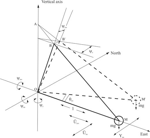
Schematic view of a garden-gate pendulum. θ_ns is the rotation angle, assimilable to a translation Y_ns according to the north–south sensitivity axis of the sensor. This rotation θ_ns can be generated by translations and also by rotations ψ_ew around the east–west axis and around the vertical axis. Rotation ψ_ns around the north–south axis changes the pendulum period, and the disturbances according to this degree of freedom are negligible compared to the signals of translations and rotations. The OBM pendulum moving part is strictly in the OAM plan. The displacement from B to B′ under the effect of the tilt ψ_ew, imposes a gap from M to M′. The rotation ψ_z acts in the same way as the translation .

Open in new tabDownload slide

• (i)

  The first degree of freedom that we will consider is the horizontal translational motion of the mass that defines the sensitivity axis of the sensor. This is precisely equivalent to a small θ_ns angle of rotation around a quasi-vertical axis that has a very large radius compared to the displacements that are to be detected. This approximation is perfectly valid and gives us the horizontal NS displacement Y_ns.

• (ii)
  The second degree of freedom, denoted as ψ_ns, is a rotation around the north–south horizontal axis, parallel to the sensitivity axis of the sensor. This rotation changes the angle that forms the two points of the pendulum fastener with the vertical. This angle controls the period of the pendulum and practically speaking, small rotations around this degree of freedom will not disturb the translation measurements because the sensitivity of the period to this angle is very low. This angle defines the so-called period foot, and thus it controls the period T₀ of the pendulum through the relation:

  

  1

  where the gravity is denoted by g. The length of the equivalent pendulum can be considered as the quantity d/ψ_ns.
• (iii)

  The next degree of freedom is a rotation ψ_ew according to an orthogonal horizontal axis to the pendulum sensitivity axis. This rotation is in the horizontal plane and acts on the angle between the two points of the pendulum fastener and the vertical (just as for the previous case, but within a perpendicular plane). This rotation moves the highest point of the pendulum fastener and induces a change in the mass balance position. For a short-period instrument, the mass sensitivity to this rotation is not very important. When the period of the pendulum becomes larger, this sensitivity increases, until the stability of the pendulum breaks down. This angle defines the so-called centring foot, which allows the installation of the apparatus. The first degree of freedom θ_ns will increase proportionally with respect to the angle ψ_ew and decrease with respect to the angle ψ_ns.

• (iv)

  The fourth degree of freedom of this type of pendulum is a rotation around the vertical axis, denoted as ψ_z. We have distinguished between this rotation around the vertical axis of the frame and the θ_ns angle related to the oscillation of the mass that has been assimilated to the translation Y_ns. In other words, this radial excitation will perturb the first degree of freedom Y_ns as any translation acceleration .

By summarizing previous studies (Rodgers 1968; Bradner & Reichle 1973; Trifunac & Todorovska 2001; Graizer 2005, 2006b), and for all garden-gate pendulum, we can write the differential equation followed by the measurable parameter Y_ns through the expression:

2

As shown in eq. (2), the ordinary differential equation gives us the first order Y_ns translation according to three right-hand side excitation terms: two rotations, ψ_ew and ψ_z, and one translation, U_ns. Standard approximations will cause us to neglect exciting terms except that of the translation U_ns that we are interested in recovering. We have neglected the cross-axis term related to the acceleration term according to the EW axis. The electronic feedback of the system maintains the mass in the balance position, which makes this term negligible.

It should be stressed that to the first order, Y_ns depends on the tilt ψ_ew, a feature well known to manufacturers: they use this tilt for the calibration of their sensors (Streckeisen 1983).

A similar equation exists for an EW horizontal sensor, with the following equation for the recorded signal Y_ew through the expression:

3

where we must consider the new rotational degree of freedom ψ_ns. The rotation ψ_z is acting the same way on this EW sensor as it does on the NS sensor, an identical excitation that we will consider for the interpretation of microseismic noise, which is similar on both of the horizontal components of seismic sensors.

By taking the Laplace transform of the eq. (2), we end up with the equation:

4

which shows that the sensitivity to both translation U_ns and rotation ψ_z is identical in the entire frequency range, similar to a second-order high-pass filter defined by:

The sensitivity to the tilt, ψ_ew, can be written as:

For a long-period pendulum, this term of the tilt becomes very important, with the sensitivity of this pendulum being highly sensitive to this tilt (Fig. 2). On the modern apparatus, the use of electronic feedback makes the significant increase in the natural period T₀ possible. As the effect of the tilt depends on the square of the period T₀, the effect of the tilt ψ_ew will rapidly become important for long periods.

Figure 2

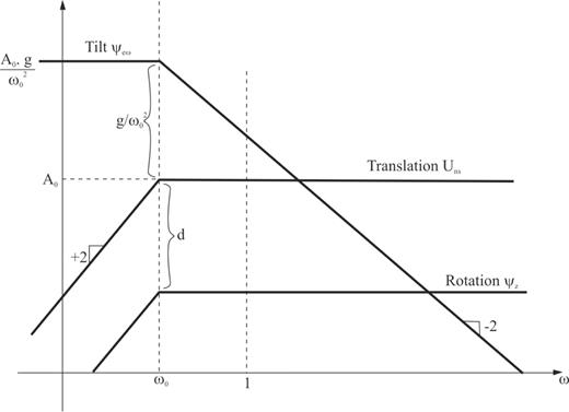
Log–log frequency response asymptote of rotations and translational sensitivity for a horizontal garden-gate pendulum. The ψ_z bandwidth is proportional to the factor d for the classic seismometer bandwidth. In the case of sensors with electronic feedback, the value of ω₀ can be very small and the effect of tilt largely amplified at long periods. The seismic recordings are the sum of these three inseparable contributions.

Open in new tabDownload slide

We have repeated the results of Rodgers (1968) for frequency bandwidth estimation of the two degrees of sensitivity related to translation (noting that the rotation ψ_z is neglected) and tilt ψ_ew of a horizontal sensor (Fig. 2). Therefore, detection of the strongest contribution between U_ns and ψ_ew is possible either in the frequency domain or in the time domain (Bradner & Reichle 1973). However, generally, the rotation ψ_z cannot be distinguished from the translation U_ns and should be measured by other means.

2.2 Vertical pendulum analysis

Let us now consider a vertical geophone designed as a cylindrical mass guided in its translation by six elastic fasteners (piano wire), as mentioned previously. We will draw similar results for the designs proposed by Galitzine/LaCoste. The mass of the vertical sensor is maintained in the equilibrium position by a spring. The first panel of Fig. 3 shows a vertical geophone, while the second panel presents a geophone tilted by an angle ψ₁ at rest, with a static deficit force equal to mg cos ψ₁ when compared with the perfectly vertical geophone. When the sensor suffers ground motion, we can consider the third panel of Fig. 3, with an absolute tilt angle ψ₂. The rotation ψ_tilt=ψ₂−ψ₁ must be considered in the equation of the motion of the mass. To do so, we must take into account the deficit force related to this tilt, and therefore, the cosine effect up to the second order (Streckeisen 1983), often taken as a negligible quantity (Graizer 2005, 2006b). The general equation of the vertical pendulum can be written as the following expression:

5

The first-order approximation with respect to the incremental rotation ψ_tilt appears by simply assuming this rotation to be small with respect to the static initial angle ψ₁, leading to the first-order equation written as:

6

For active sensors, the feedback system will lead to this equation without any approximation. This equation shows the complex excitation coming from the tilt angle for the mass motion V_z. Ideally, these excitations should be negligible with respect to the acceleration . Often, only the tilt acceleration term has been considered when assuming a perfectly vertical installed sensor with an angle ψ₁≈ 0.

Figure 3

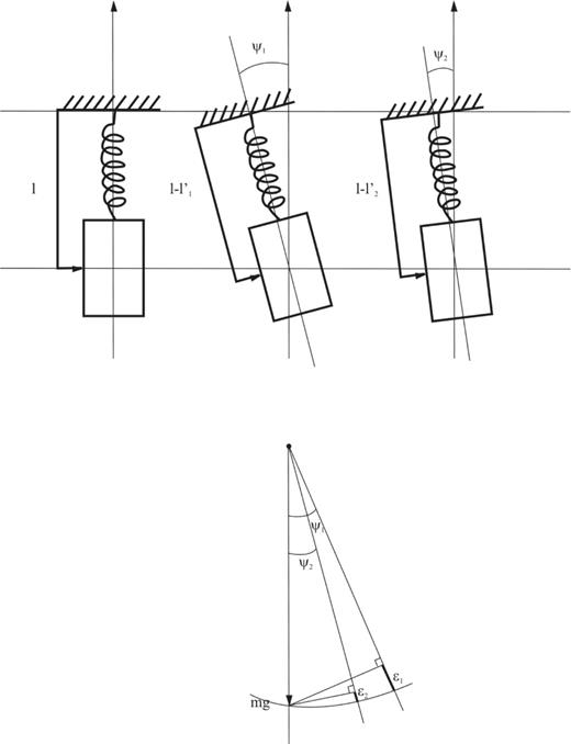
Schematic view of a strictly vertical geophone, and the same tilted from ψ₁ and from ψ₂. The projection of the weight of the mass along the sensitivity axis changes according to the tilt.

Open in new tabDownload slide

The installation using a bubble level protocol does not allow the necessary precision (the precision needed is about 0.1 μ rd for an accelerometer). The lowest position of the pendulum mass is obtained when the sensor is perfectly vertical. This information must be used for the installation of vertical seismometers. We should note that this installation protocol is used for the installation of LaCoste-Romberg gravimeters of the IDA project (Agnew 1986), with an angular precision of around 10⁻¹² rd. If the installation is well carried out, we can neglect both the linear and the quadratic terms related to the rotation ψ_tilt.

We can apply the Laplace transform to the linearized eq. (6), which gives us the following equation:

7

When considering a perfectly vertical sensor, both the translation term and the tilt term provide the same bandwidth response as for the horizontal sensor. By considering an initial statically tilted sensor, the tilt term has a more complex frequency response as:

which illustrates the difficulties when a sensor is not installed properly.

Difficulties in the double integration of the vertical acceleration can be related to this tilt change, which is more difficult to identify than tilt changes related to horizontal accelerations. The absence of an absolute reference frame for horizontal-sensor orientation implies a relative tilt measurement by opposition to the vertical sensor, for which the gravity introduces an absolute direction to which the tilt change is sensitive.

We mostly work in seismology with linear accelerations of the ground, and we have seen that we have to neglect contributions of rotations, or, in other words, we must consider a zero antisymmetric part of the differential displacement tensor. However the sensors are installed, we have seen that this approximation is no more valid in the near field or at the very long periods, as sensors increase their sensitivity. We must reconsider our instrumentation to estimate these rotational effects in the future. We will now examine a few examples where we can note unambiguous influences of rotation.

3 NEAR FIELD ILLUSTRATIONS

Static displacement estimation has been investigated from a theoretical point of view by Poincaré (1888) and Lippmann (1890) through the integration of a theoretical seismogram. In practice, the double integration of Cartesian acceleration rarely leads to acceptable results: the estimation of a zero baseline is required (Trifunac 1971; Boore 2001; Boore 2002) and difficulties in doing so make integrated signals diverge. These instabilities have often been associated with the narrow frequency band of accelerometers. As the instrumentation design has been improved, with an extension to the DC level for accelerometer response, incomplete reconstructions of the static displacement can only be related to the sensitivity limit of these new broad-band accelerometers. For large earthquakes, such as the Chi-Chi earthquake (Mw 7.6) that occurred in Taiwan on 1999 September 20, the motion quickly reaches a significant level, and therefore, the discrepancy with GPS measurements needs another explanation than a possible low sensitivity at long periods (Fig. 4).

Figure 4

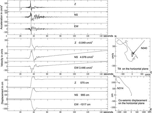
Chi-Chi earthquake (Taiwan, 1999 September 20; Mw 7.6) recorded at the TCU068 accelerometric station of the TSMIP network (Taiwan Strong Motion Instrumentation Programme). The first three traces show the original acceleration signals in cm s⁻². The velocity signals are obtained by time integration. The obvious slopes (−0.049, 4.076 and 3.446 cm s⁻² for Z, NS and EW component) are the evidence of hidden jumps in the acceleration signal. The plotted velocity particule motion in the horizontal plane clearly shows the tilt azimuth (N40°). Tilt amplitude (5.44 mrad) is deduced from the horizontal component acceleration jumps. After removing the acceleration jumps from the acceleration signals, the double time integration can be performed without a break in the baseline and gives very acceptable coseismic displacement traces, although the reading values (575, 995 and −1017 cm for Z, NS and EW components, respectively) are over-evaluated in comparison with GPS measurements. The plotted coseismic displacement in the horizontal plane shows a N 314° of azimuth, in agreement with the Chi-Chi earthquake focal mechanism.

Open in new tabDownload slide

In the near field, significant rotations disturb the accelerometer recordings (Boroschek & Legrand 2006; Graizer 2006a). The slopes produced by the vertical coseismic displacement field give tilt values that are too low compared to observations generally made in the near field. Berg & Pulpan (1971), McHugh & Johnston (1977), Wyatt & Berger (1980) and Zahradnik & Plesinger (2005) have observed tilts that are two to three orders of magnitude greater than the values predicted by Bouchon & Aki (1982). Deconvolved velocity traces of the TCU068 accelerometric station (located at the northern end of the Chelungpu fault in Taïwan) of the TSMIP network show a significant break of the slope, which can be attributed to a very small jump in the baseline of the acceleration traces (Fig. 4). Very few of the traces among the 400 collected during the Chi-Chi event restore an acceptable static displacement. Indeed, the majority of the recordings must be corrected to reach coherent static displacement estimations, in agreement with values given by the colocated GPS stations.

Let us consider the three components of the accelerometer of the TCU068 station of the network TSMIP. First of all, the slope of the recorded noise before the P-wave arrival time is estimated and subtracted from the signal (Fig. 4). Then, the jumps in the acceleration with respect to this baseline can be estimated using the last 30 per cent of the signal and can be expressed in cm s⁻². We found −0.049 cm s⁻² for the vertical one, 4.077 cm s⁻² for the NS component, and 3.446 cm s⁻² for the EW component. The first integration leads to the particle velocity, which is expressed in cm s⁻¹. The observed slope is related to the acceleration jump that we have measured. We can subtract this from the acceleration records before the integration, assuming that the acceleration jump starts when the velocity slope crosses the horizontal axis for each signal. Of course, this intersecting time should not occur before the P-wave arrival time. By doing so, we may proceed to the next integration and reconstruct the displacement signal: a static displacement can be measured easily without divergence of the traces, and it turns out to overestimate that deduced from different observational studies (Boore 2001; Ma 2001; Oglesby & Day 2001). A static displacement of more than 13 m is estimated at the TCU068 station, whereas close-by GPS measurements give only 10 m. The difference between the unknown rotational signal and the jump approximation used for this correction can explain this discrepancy. More complex corrections have been proposed from many studies (Trifunac 1971; Boore 2001; Boore 2002), but to date we must rely mainly on geodetic measurements for reliable estimations of static displacement (Wang 2003, 2007).

This raw correction of the accelerometric signal illustrates a good strategy for reconstruction of the dynamic and static coseismic displacement. Of course, a correct value of the true rotational signal should be provided, and not the one we have used as deduced from the seismic signal.

The tilt signal appears very clearly on the velocity trace as a linear drift, after the first integration. The slope measurement of this velocity signal makes it possible to know the height of the jump on the acceleration trace: another way to estimate the acceleration jump. The full temporal window of 3 min is sometimes too short for reliable estimations of slopes, as the pre-event of 18 s makes the baseline estimation difficult as well. We may consider that the value dispersion in the estimation of slopes arises from these shortcomings.

GPS stations give displacement values without ambiguity, and an increase in the sampling of GPS measurements up to 10 Hz or more can provide a dynamic measurement of the coseismic displacement. The uncertainty of GPS processing is still too important and does not provide the accuracy we wish to have for the analysis of ground motions related to earthquakes. We may need to record rotations in order to correctly subtract these signals from seismic traces and to accurately cancel the influence of tilt. This will provide us with high-resolution dynamic displacement in the near field, which could be useful information.

The slopes of horizontal velocity traces measure the static part of the tilt and it becomes possible to measure the amplitude and azimuth of this tilt. By doing so for the accelerometer network of Taiwan following the Chi-Chi earthquake, we find quite different tilt amplitudes that are dispersed over several orders of magnitude. The tilt azimuths do not show any general pattern as has often been seen (Berg & Pulpan 1971; McHugh & Johnston 1977; Wyatt & Berger 1980). Again, only accurate rotation recordings can solve this difficulty and give us this potentially interesting information on the tilt distribution around a seismic fault.

The Chi-Chi earthquake was an opportunity for the investigation of tilt because more than 400 accelerometer stations on the Taïwan island recorded clean signals. This analysis has shown that we need additional information for better interpretation of the seismic effects.

From the three acceleration jump measurements, we can calculate the TCU068 tilt at the installation of the sensor by considering that these are pure effects that are due to rotations through the expression:

8

The tilt ψ_tilt should be calculated by combining the values of the two horizontal components: we found the value 5.44 × 10⁻³ rd for the N 40° azimuth. Finally, the TCU068 starting tilt ψ₁ has a value of 1.2 × 10⁻² rd, which is equivalent to an angle variation of 0.68°. We will see later that these measurements are compatible with our laboratory observations.

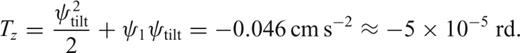
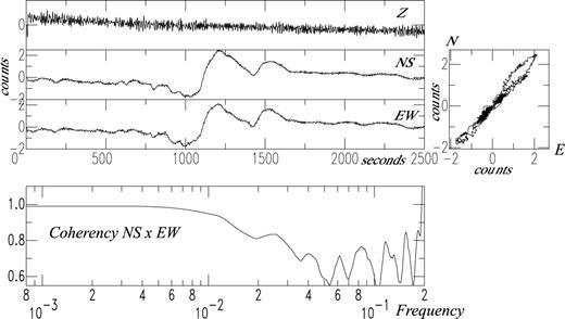
Similarly, as the feedback loop of active velocimeters has been improved, there is the chance of recording unclipped signals on velocimeters for important earthquakes at rather short distances. Deconvolution of these particle velocity records by the instrument response also leads to unfiltered long-period acceleration with unexplained baseline jumps (Berckhemer & Schneider 1964; Zahradnik & Plesinger 2005). These jumps have often been explained as instrument calibration problems at long-period ranges, and have often been disregarded by filtering the seismic signals. Previous comments about accelerograms tell us we should reconsider these signals for a more careful analysis. Tilt observations on velocimeters can be detected in the narrow frequency band delimited by the sensor saturation and the coseismic tilt attenuation. Broad-band velocimeters installed in seismogenic zones can record strong magnitude earthquakes at small epicentral distances. Raw recordings do not show particular features (Fig. 5a), except when the signal is quite strong, and then the recording becomes asymmmetric (Zahradnik & Plesinger 2005). When, by chance, the signal is not saturated, its deconvolution of the instrument response in acceleration shows jumps in the baseline (Fig. 5d), due to the long-period content. As velocimeters have a higher sensitivity than accelerometers, the jump in the deconvolved acceleration is quite visible on the signal (Fig. 5d). The apparent trace of the raw uncorrected velocity signal does not show this drift (Fig. 5c), except for the vertical component, as the instrument response is not flat at long periods. The long period part of the integrated raw signal (Fig. 5b) looks like an acceleration signal. The jumps in the deconvolved acceleration of the horizontal components have previously been interpreted as tilts (Berckhemer & Schneider 1964; Zahradnik & Plesinger 2005).

Figure 5

Broadband near-earthquake recording example: earthquake from October 3, 1998, at 16h 42 mn; Mb 4.1, 16.670S, 167.506E, superficial (NEIC informations) recorded at SWB station (South West Bay, 16.5087S, 167.4203E, Malicolo, Vanuatu) on a Güralp CMG3-ESP broad-band seismometer. The epicentral distance is about 25 km. (a) Seismic traces of the three components. Nothing appears on the recordings. (b) The same traces after time integration. At long period, below T_o (100 s) the signal looks like an acceleration one and the acceleration jumps can be seen. (c) Seismic traces deconvolved for velocity. The slope is very strong in the vertical component, showing clearly that the seismometer is not vertically installed. The traces are filtered by a 1-Hz low-pass filter to reveal the drifts. (d) Seismic traces plotted for the acceleration after a 0.1 Hz low-pass filter. Acceleration jumps are quite visible.

Open in new tabDownload slide

For this specific example, we can conclude that the Güralp CMG3-ESP sensor of the station SWB has a significant initial tilt, giving great importance to the excitation term g ψ₁ψ_tilt (eq. 6). The high broad-band sensitivity of this sensor makes possible measurements of very small amplitude tilt. As for the accelerometers, possible coseismic static displacement recording is hidden by the recording of tilts amplified by the broad-band velocimeter.

4 FAR-FIELD ILLUSTRATION

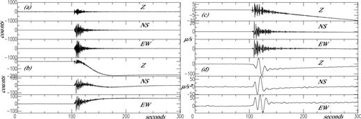
In seismometry at very long periods, that is, between a few hours and approximately 50 s, the two horizontal components of the same broad-band station sometimes show very similar signals for the background noise. In other words, the two components appear strongly correlated in phase and in amplitude, as if the background noise projects identically on these two horizontal directions. Coherence between these signals is sometimes higher than 95 per cent in this period range (Figs 6 and 7). The representation of the particule motion in the horizontal plane clearly shows this polarization along the N45° azimuth. While the sensor only records translational components, this observation is unexpected as the background noise cannot have a permanent 45° azimuth.

Figure 6

Twenty-four hours (January 10, 2004) of background noise components at the PPT (STS-1, Pamataï, Tahiti) GEOSCOPE station. The horizontal traces after the velocity deconvolution are very similar. The particule motion in the horizontal plane is 45° of azimuth polarized and the coherence between the two horizontal signals is approximatively 95 per cent. The horizontal trace amplitude is approximatively 1 μm s⁻¹ peak-to-peak, corresponding to a rotation of 10 μrad s⁻¹ (we took an arm length of 10 cm).

Open in new tabDownload slide

Figure 7

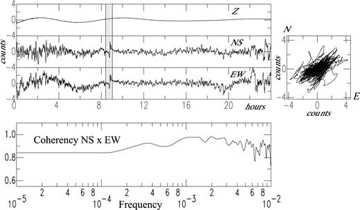
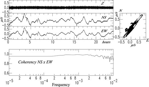
The same as previous Fig. 6 for the NOUC GEOSCOPE station (STS-1, Nouméa, New Caledonia). The signal is not deconvolved from the apparatus response, but it is filtered between 10⁻⁴ and 10⁻² Hz. The coherence of the two horizontal components and the polarization of the particule motion in the horizontal plan are less obvious than at the PPT station, but the rotation ψ_z has a strong visible effect. The shaded box is enlarged in Fig. 8.

Open in new tabDownload slide

By taking into account the influence of the ψ_z rotation around the vertical axis on horizontal components, we can draw up a simple explanation of this phenomenon: the ψ_z rotation acts in the same way on the two horizontal components (see eqs 2 and 3). These two components have their rotational vertical axis at a distance less than 1 m away. For long periods, we can assume that the two pendulums undergo the same vertical rotation and that the related signals that are recorded have the same amplitude and phase on both of the horizontal components.

As an illustration, at the PPT (Pamatai, Tahiti) station of the GEOSCOPE network (Romanowicz 1991) equipped with a STS-1 sensor (Wielandt & Streckeisen 1982), we analysed 24 hr of long-period (over 100 s) noise recorded on 10th January 2004: the horizontal components show very similar traces, with a correlation coefficient higher than 95 per cent (Fig. 6). The stability of this horizontal polarization of 45° is quite impressive and leads us to conclude that the two horizontal components are sensitive to the same time-varying parameter. We suggest that the ψ_z rotation is this parameter.

At the PPT GEOSCOPE station, we measured a peak-to-peak amplitude of 1 μm s⁻¹, giving a rotational velocity of 10 μrad s⁻¹ in amplitude by taking the length of the arm of the seismometer with a value of 10 cm. The entire year 2005 has been examined, and the rotation ψ_z noise shows a quite stable amplitude over the year.

For the 10th January 2004, we checked that the stations of the GEOSCOPE network equipped with a STS-1 sensor show similar polarization, although the polarization amplitude can vary. At a given station, we can consider that the translational noise might hide this ψ_z rotational noise from time to time.

For the GEOSCOPE network, stations equipped with a STS-2 sensor do not show this N45° polarization, as the specific design of this sensor with three 120° tilted arms makes this sensor insensitive to the ψ_z rotation (Melton & Kirkpatrick 1970). The horizontal components and the vertical components are recombined analogically from the physical recorded tilted components. This very wise design only needed the construction of one mechanical oscillator.

Finally, the exceptional recording of six degrees of freedom in the near-field of a chemical explosion by Nigbor (1994) shows a strong correlation between rotational velocity along the x direction and the translational acceleration in the y direction (see Fig. 4 of the original paper): this shows the influence of the tilt perpendicular to the measured translational component.

Fig. 8 shows an unexplained episode observed at the NOUC (Nouméa, New Caledonia) station of the GEOSCOPE network: no seismic event related to this disturbance was reported in the NEIC bulletin. We can speculate that this signal could be related to a local ψ_z rotational event, which was particularly well polarized at periods higher than 100 s as shown by the coherence between the two signals.

Figure 8

An unforeseeable event at the NOUC GEOSCOPE station (STS-1, Nouméa, New Caledonia) 10 January, 2004, at 8 h am 28 mn (start time of the window). The 40 min time window of the horizontal signals (nothing appears on the vertical component) shows a perfectly polarized signal in 45° of azimuth with a coherence (between the two horizontal traces) higher than 95 per cent. No seismic event appears to be connected with this disturbance, which may have a local origin.

Open in new tabDownload slide

5 LABORATORY EXPERIMENTS

The influence of the rotational motion around the vertical axis can be reproduced in a very simple laboratory experiment. We can install a sensor on a rotating table along the vertical. First, we must install the Episensor FBA ES-T accelerometer from Kinemetrics with the careful checking of the verticality of the sensor, as mentioned previously. The output voltage is measured using a voltmeter with an accuracy of 1/100 mV. The three screws of the adjustable rotating table make modification of the horizontality of the sensor possible: we reach the maximum tension corresponding to a zero tilt by varying screw positions. We note that the position selected did not correspond exactly to the position given by the bubble level.

Once the sensor was properly installed, a light periodic motion was applied to the rotating table and the signals are recorded by the sensor. Fig. 9 shows that the two horizontal components record exactly the same signal, which is 100-fold larger than the background noise on the vertical component. The horizontal signals appear to be produced by a translational wave polarized to 45°, as we expected from our analysis.

Figure 9

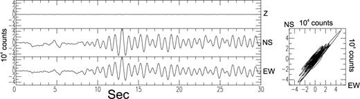
Laboratory test of an Episensor FBA ES-T accelerometer from Kinemetrics on a rotating table. The long-period part (>1 s) of the raw signals of the horizontal traces are identical in amplitude and phase, giving the impression of a translational wave polarized to 45° of the two horizontal components.

Open in new tabDownload slide

For a better appreciation of the influence of the installation, we bring the accelerometer back to the position defined by the bubble-level position. This operation gives an idea of the effect of improper installation. Here, the installation error was about 2.3 mrd. This important error of the sensor verticality prevents the neglecting of the effect of the coseismic tilt in the seismic records: a coseismic tilt correction should be performed. Therefore, we need to measure tilts by other means.

6 CONCLUSIONS

We have shown that the inertial sensors used for the measurement of ground translations by the seismologist community are also sensitive to rotations. The output signal of the sensor is a combined mixture of translations and rotations. The static component of horizontal rotations is often labelled as tilt.

These often unnoticed rotations become quite dominant in the near field and in the seismic long-period background noise everywhere. In the near field, tilt effects prevent the measurement of the coseismic translation displacements. Therefore, we recommend a protocol of installation with a careful check of verticality for vertical sensors. This protocol will need an accuracy better than that given by the bubble technique. We can also underline the need for independent tilt measurements with sensors dedicated to these rotational quantities. If so, we can correct the translation signals from these rotations to recover the full correct displacement history.

We can speculate from measurements that we have performed that the distribution of the coseismic tilts around the rupture zone is quite complex and may be a superposition of various effects such as the horizontal gradient of the coseismic vertical displacement field, a coseismic tilt directly generated by the source, a fluid redistribution to a shallow depth that can modify the local gravity, or potentially other explanations that we have not thought of.

The influence of the ψ_z rotation around the vertical axis is clearly shown in the horizontal components of the GEOSCOPE stations equipped with horizontal STS-1H sensors of garden-gate design, built by Streckeisen (1983).

ACKNOWLEDGMENTS

We thank Heiner Igel and an anonymous reviewer for their helpful comments which broaden the impact of your analysis of hinged pendulum.

REFERENCES