


Summary
The Queen Charlotte Fault zone is the transpressive boundary between the North America and Pacific Plates along the northwestern margin of British Columbia. Two models have been suggested for the accommodation of the ∼20 mm yr−1 of convergence along the fault boundary: (1) underthrusting; (2) internal crustal deformation. Strong evidence supporting an underthrusting model is provided by a detailed teleseismic receiver function analysis that defines the underthrusting slab. Forward and inverse modelling techniques were applied to receiver function data calculated at two permanent and four temporary seismic stations within the Queen Charlotte Islands. The modelling reveals a ∼10 km thick low-velocity zone dipping eastward at 28° interpreted to be underthrusting oceanic crust. The oceanic crust is located beneath a thin (28 km) eastward thickening (10°) continental crust.
1 INTRODUCTION
The current tectonic setting and seismicity of the Queen Charlotte margin are dominated by the Queen Charlotte Fault zone (QCF), the transpressive boundary between the Pacific and North America Plates along the northwest margin of Canada (Fig. 1). The relative Pacific/North America motion along the fault zone is primarily right-lateral transform at a rate of ∼50 mm yr−1; however, there is also a significant component (∼15 mm yr−1) of convergence across the margin (e.g. DeMets & Dixon 1999; Kreemer 2003). Convergence along the QCF is confirmed by northward margin-oblique GPS velocities (Mazzotti 2003; Bustin 2006) and thrust faulting mechanisms for earthquakes along the southernmost section of the fault (Bird 1997; Ristau 2004).
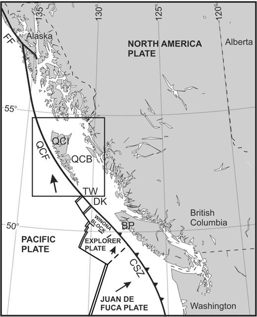
The location of the Queen Charlotte Fault zone with respect to neighbouring plate boundaries; black box shows the location of Fig. 2; FF, Fairweather Fault; QCF, Queen Charlotte Fault; QCI, Queen Charlotte Islands: QCB, Queen Charlotte Basin; CSZ, Cascadia Subduction Zone; TW, Tuzo Wilson seamounts; DK, Dellwood Knolls; BP, Brooks Peninsula.
Two end-member plate models have been proposed for the convergence along the QCF based on the geophysical and geological characteristics of the Queen Charlotte margin. In the first model, margin-parallel motion is accommodated by strike-slip motion on a nearly vertical QCF and convergence is taken up by internal deformation and shortening within the Queen Charlotte Terrace and in the adjacent Pacific and North America Plates (e.g. Rohr 2000). The second model involves underthrusting of a Pacific slab beneath the overriding North America Plate either obliquely beneath the margin or orthogonally, separated from the Pacific Plate by a transform QCF cutting through the slab (e.g. Yorath & Hyndman 1983; Hyndman & Hamilton 1993).
The Queen Charlotte Islands (QCI) area is one of Canada's most seismically active regions. The QCF produced the country's largest historically recorded earthquake, a magnitude 8.1 strike-slip event in 1949. Additional significant strike-slip earthquakes along the fault zone include two magnitude ∼7 events near the southern tip of Moresby Island in 1929 and 1970. The confirmation of underthrusting in the Queen Charlotte region could introduce an additional component to the seismic hazard on the west coast of Canada. If underthrusting is occurring along the Queen Charlotte margin then great thrust earthquakes and associated tsunamis may also be expected.
A teleseismic receiver function analysis was conducted at six three-component broad-band stations that cross the QCI in order to constrain the crustal structure and resolve whether the oblique convergence is accommodated by crustal thickening or underthrusting beneath the Islands. Receiver functions were calculated from the data recorded at the two permanent seismic stations on the QCI, Moresby (MOBC) and Dawson Inlet (DIB), as well as at four temporary stations that were installed for the Nuclear Test Ban Treaty studies during the summer of 1999 (Fig. 2). Inverse and forward modelling techniques were applied to the receiver functions to provide constraints on the crustal structure and thickness, as well as to determine whether an underthrusting slab is present. This study follows initial receiver function work for MOBC by Smith (2003), which used 3 yr of data at MOBC. The new study includes 9 yr of data at MOBC, 2 yr at DIB and 3–12 months of data at the temporary sites.
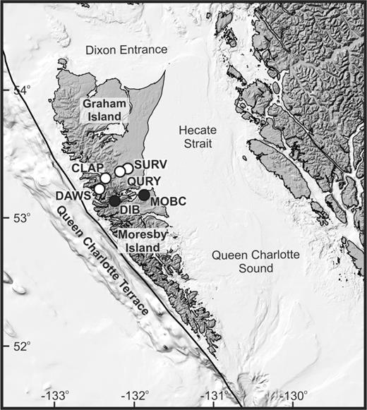
The location of the permanent (black) and temporary (white) seismic stations used in the teleseismic receiver function analysis of the Queen Charlotte margin.
2 TECTONIC SETTING
The plate boundary between the oceanic Pacific Plate and the continental North America Plate along the central west coast of British Columbia is the QCF. The QCF is one of the few locations in the world where there is a transition from oceanic to continental crust across a major plate boundary. The main QCF is located immediately offshore the QCI and extends northwestward at ∼320° from the triple junction at the northern extreme of the Cascadia subduction zone to the Fairweather Fault off the west coast of Alaska (Fig. 1).
The current relative plate motion between the Pacific and North America Plates (Engebretson 1984; Stock & Molnar 1988; DeMets 1990; DeMets 1994; Norton 1995; DeMets & Dixon 1999; Kreemer 2003) increases northward along the QCF from ∼46 to 48 mm yr−1. The relative plate motions differ significantly from the strike of the Queen Charlotte margin, indicating a component of convergence between the Pacific and North America Plates. The amount of current convergence varies along strike of the margin from ∼20 mm yr−1 in the south to ∼12 mm yr−1 in the north due to variations in the angle between the relative plate motion and the strike of the fault. The continuation of the QCF further to the north (Fairweather Fault) has a similar trend to the relative plate motion vectors and is therefore nearly purely transcurrent. The current transpressive regime was initiated ∼5 Ma with an uncertainty between 3 and 9.8 Ma (Cox & Engebretson 1985; Harbert & Cox 1989; Atwater & Stock 1998). Estimates of the total amount of convergence along the Queen Charlotte margin vary from 80 to 160 km depending on the duration of the convergence and the assumed location of the triple junction since the start of convergence.
The western QCI contains a 50 km wide range of mountains parallel to the plate boundary with elevations exceeding 1000 m. The mountains do not appear to be due to crustal shortening and thickening. There is no evidence of recent shortening in the geological structure (e.g. Sutherland Brown 1968; Thompson 1991) and seismic refraction data indicate a normal to thin crustal thickness (e.g. Horn 1984; Dehler & Clowes 1988; Mackie 1989; Yuan 1992; Spence & Asudeh 1993; Spence & Long 1995). Immediately offshore the west coast of the QCI there is a narrow (<10 km wide) continental shelf which drops steeply to a 30-km wide terrace (the Queen Charlotte Terrace; Fig. 2) at a depth of ∼1.5 km (Riddihough & Hyndman 1989). The outer edge of the terrace is bound by a second scarp that steeply drops to depths of 2.5–3 km into the sediment-filled Queen Charlotte Trough. Seismic profiling (Horn 1984), seismic refraction (Dehler & Clowes 1988; Mackie 1989), heat flow (Hyndman 1982) and gravity interpretation (e.g. Sweeney & Seemann 1991) of the fault-bound terrace suggest that it is composed of high amplitude folds of marine sediments up to 5 km thick that were accreted to the margin forming an accretionary prism. The trough probably formed in response to lithospheric loading of the Pacific Plate by the obliquely overthrusting North America Plate and by the sediments of the terrace and trough (e.g. Hyndman & Hamilton 1993; Prims 1997). The deep sea basin sedimentary horizons dip into the trough suggesting oceanic plate downwarping.
The morphology of the Queen Charlotte margin is characteristic of many subduction zones, suggesting the presence of underthrusting. Additional evidence supporting an underthrusting model for the accommodation of convergence across the plate margin includes: a parallel free-air gravity low-high anomaly pair characteristic of subduction zones (Riddihough 1979), elastic flexural modelling (Prims 1997), thermal modelling (Smith 2003), forward modelling of receiver functions (Smith 2003) and the lack of evidence of substantial crustal thickening or deformation (e.g. Spence & Asudeh 1993). The main argument against an underthrusting model is the absence of clearly recorded Wadati–Benioff earthquakes within an underthrusting slab. However, the recent initiation of transpression and the high heat flow along the margin due to a hot young oceanic crust may inhibit brittle failure or limit intraslab seismicity to very shallow depths beneath the Queen Charlotte Terrace and the western coast of the QCI. In addition, the seismic refraction and gravity modelling across the Queen Charlotte margin have been unable to resolve the deep velocity structure such as to discriminate between plate models with and without an underthrusting slab (e.g. Spence & Asudeh 1993; Spence & Long 1995).
3 DATA AND ANALYSIS
Teleseismic receiver function studies use seismic data from large distant earthquakes recorded at three-component broad-band seismographs to provide site-specific constraints on the underlying S-wave velocity structure of the crust and upper mantle (for a detailed explanation of this technique refer to Langston 1977; Owens 1984; Ammon 1991; Cassidy 1992). A receiver function is a time-series corresponding to the complex spectral ratio of the horizontal-component (radial or tangential) to vertical-component seismograms. Deconvolving the vertical from the horizontal seismograms removes the effective source time and instrument impulse responses leaving only the receiver's response to the earth structure. The deconvolution suppresses all P-wave arrivals except for the direct P-arrival, but leaves all P-to-S (Ps) conversions and reverberations since they are almost exclusively on the radial component of the ground motion. Thus, the arrivals on a receiver function include the direct P-arrival, locally generated Ps phases and crustal multiples, which are displayed as peaks and troughs.
The amplitude of the converted phases is determined by the S-velocity contrast between layers and the incidence angle of the impinging P-wave. The arrival time is a function of the average velocity and the depth of the interface and the polarity of the arrivals indicates whether the impedance contrast is positive or negative. Energy on tangential receiver functions is normally very small, although in the presence of a dipping interface or anisotropy, the P- and S-waves from the radial-vertical plane are partly rotated into the tangential plane. The cross-strike arrivals from a dipping interface will have very little tangential energy while the along-strike arrivals will have significant energy and a polarity reversal. A maximum amplitude positive arrival will occur in the direction 90° clockwise from the dip direction and a maximum negative arrival will occur in the direction 90° counter-clockwise from the dip direction (Cassidy 1995a,b). Therefore, the tangential component for a dipping structure will be characterized by mirrored arrivals across a line parallel to the dip direction.
Similarly to dipping interfaces, teleseismic wave propagation through anisotropic media results in variations of traveltimes and amplitudes with backazimuth, as well as the rotation of energy onto the tangential receiver functions (e.g. Savage 1998; Frederiksen & Bostock 2000 and references therein). For hexagonal anisotropic layers, the radial receiver functions are symmetric and the tangential receiver functions are antisymmetric about the axis of symmetry. The radial receiver functions for hexagonal anisotropy with a horizontal symmetry axis exhibit a 180° periodicity about the fast and slow axes. The tangential receiver functions also display a 180° backazimuthal periodicity, with polarity reversals about the fast and slow directions where the amplitude of the transverse energy is zero. The amplitude has maximum energy for waveforms at 45° to the fast and slow directions. Transverse energy from the initial P-phase occurs for anisotropic layers only when there is an anisotropic uppermost layer, as opposed to dipping isotropic interfaces which always produce an initial arrival. The 180° periodicity of the waveforms is destroyed for anisotropy with dipping axes of symmetry. The receiver functions produced from an anisotropic layer with plunging axis may exhibit a 360° symmetry making it difficult to distinguish from isotropic dipping interfaces.
Earthquakes that occurred between distances of 30° and 90° from the QCI seismic stations with magnitudes greater than 5.5 were analysed; however, due to high noise levels on the Islands very few events with magnitudes less than 6.0 were used and most events had magnitudes greater than 6.5. The noise level at the stations is much greater during the winter with characteristic strong winds and ocean waves, so most high-quality events were during the summer months. The earthquake data recorded at the temporary stations were obtained from the Ottawa office of the Geological Survey of Canada (GSC) and the data recorded at the permanent stations are available from the Canadian National Seismograph Network (CNSN) at the GSC. The original seismograms were corrected for linear trends and offsets and long period noise was removed using a bandpass filter consisting of a four-pole Butterworth filter with corners at 0.3 and 3.0 Hz.
Gaussian width factors of 5 and 1.5 were used to calculate high (low-pass up to 2 Hz) and low (low-pass up to 0.5 Hz) frequency receiver functions using the iterative time-domain deconvolution approach developed by Ligorria & Ammon (1999). The method is based on a least-squares minimization of the difference between the observed horizontal seismograms and a predicted time-series calculated by convolving the observed vertical seismogram with an iteratively updated spike train, representing the receiver function. The misfit, which is expressed as the percentage of the observed power in the horizontal seismogram that is fit by the constructed receiver function was used to discard poor deconvolutions. The traces were stacked by performing a weighted summation of the receiver functions normalized by the number of events to suppress scattered energy and attenuate ambient seismic noise. Bounds of ∼10° in backazimuth and epicentral distance were used and weights were assigned based on the misfit.
This study used earthquake data recorded at MOBC over 9 yr from its installation in March 1996. Of the 1172 earthquakes analysed 159 produced useful receiver functions that were binned into 19 stacks. The data set contains gaps in backazimuth between 20–90° and 135–220°, but provided sufficient azimuthal variation to merit an inverse modelling approach using both the radial and tangential components. An inversion technique was employed which uses the Neighbourhood Algorithm (N/A) (Sambridge 1999) in conjunction with a 3-D ray tracing code (RAY3D; Langston 1977) that allows for the inversion of dipping interfaces.
The DIB station was installed in March 2004 approximately 25 km to the southwest of MOBC. We examined 339 earthquakes and obtained 56 receiver functions that were binned into 11 stacks, although only 4 of the stacks contained more than five traces. At the time of this study, insufficient good quality data or azimuthal coverage were available to merit an inverse modelling approach. A model for the crustal structure beneath DIB was found by forward modelling, starting with the velocity structure determined at MOBC. The synthetic seismograms were generated using a 3-D ray tracing algorithm based on the method of Langston (1977).
During the summer of 1999, six temporary seismographs were installed across Moresby Island in a line perpendicular to the strike of the QCF and operated for periods of 3 months to a year (Fig. 2). The short operational periods limit the amount of good quality data available for these sites. Four of the stations (CLAP, DAWS, QURY and SURV) produced ∼20 receiver functions that were included during this analysis. Although the data set is inadequate to warrant intensive modelling, it allowed for a few important observations on the dip of the underlying structure.
4 INVERSE MODELLING
A number of modelling techniques have been developed for receiver function analysis, including forward modelling, linearized inversions and directed global searches. Linearized methods (e.g. Ammon 1990) have been in use since the early 1980s to invert for the S-wave velocities in horizontal layers with fixed thickness. More recently, directed global searches, particularly genetic (e.g. Shibutani 1996) and neighbourhood algorithms (e.g. Frederiksen 2003) have been used to model the S-wave velocity structure. The inverse receiver function problem involves converting the information provided by a receiver function into a model of the S-velocity structure of the subsurface. The inversion is complicated by the non-linear relationship between the data and the model parameters. The traveltime of an individual Ps conversion is dependent on the depth of the interface and on the S-velocity above the interface (e.g. Ammon 1990). If the region contains dipping interfaces or anisotropy, such as the Queen Charlotte margin, then the behaviour of the seismic arrivals becomes even more complex and the non-linearity of the problem greatly increases. The presence of anisotropy and dip also increases the non-uniqueness of the problem (e.g. Frederiksen 2003). The non-uniqueness can be partially avoided by using a priori information, such as P-wave velocity models and an estimate of the Poisson's ratio (Cassidy 1995b). The starting model in this study will be based on P-velocity models interpreted from seismic refraction data (e.g. Spence & Asudeh 1993; Spence & Long 1995) and a previous receiver function study of the QCI (Smith 2003).
4.1 Theory of the Neighbourhood Algorithm
The N/A, developed by Sambridge (1999), is a derivative-free directed global search method which uses geometrical constructs known as Voronoi cells to search the parameter space. The objective of the search is to find an ensemble of models that have preferentially sampled the good data-fitting regions of parameter space, instead of a single optimal solution. The inversion begins with a set number, ns, of randomly distributed points within a bounded multidimensional parameter space. The model space is then partitioned into regions, where each region (convex polygon) is the nearest neighbourhood about one of the points as determined by a particular distance measure (this study uses a least-squares-norm).
The next step of the inversion is to calculate the misfit function for the set of ns models and select the nr Voronoi cells with the lowest misfits. In each iteration, a new set of ns models are generated by performing a uniform random walk generated using a Gibbs sampler in each of the selected Voronoi cells. Forward modelling is then performed for each model and the misfits are calculated. The nr cells with the lowest misfit are chosen out of the entire set of cells and their neighbourhoods are used in the next iteration.
4.2 Description of inversion code
In this study, the well-tested RAY3D forward modelling program was adapted to run as a subroutine within the N/A search method of Sambridge (1999). During the forward modelling stage of the inversion the synthetic seismograms are deconvolved using the source equalization method (Langston 1979). The code permits velocity gradients for horizontal layers and allows the orientation (i.e. strike/dip) of a group of interfaces to be constrained as the same.
During the inversion, the misfit between the resulting synthetic and observed receiver functions were calculated using a least-squares-norm misfit function, based on the correlation coefficient between real and synthetic receiver functions. The receiver functions were weighted depending on the number of traces per stack and both receiver function components were included in the inversion with the misfits calculated, using a weighting of 1.0 for the radial component and 0.5 for the tangential component. The inversion performed 1000 iterations, using a sample size, of 36 models (ns) and retaining 18 models per cycle (nr). The parameters specified in the inversion include: layer thickness, S-wave velocity, orientation of dipping interfaces, density and the ratio of P- to S-wave velocity (Vp/Vs).
4.3 Synthetic tests
The inversion code was tested using synthetic data to verify that the technique could recover dipping S-velocity interfaces (Bustin 2006). A 5-layer model was constructed containing a layer dipping 20° to the east. Background noise was added to the synthetic seismograms by adding random numbers to the spectrum at each frequency, resulting in average noise that is 30 per cent of the peak amplitude of the signal. The inversion contained 13 free parameters, the thickness and S-velocity of each layer, as well as the orientation of the dipping interfaces, which were constrained to be the same. The recovery was good; however, a partial trade-off was observed between velocity and layer thickness, reflecting the sensitivity of Ps-conversion traveltimes (Fig. 3).
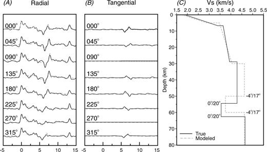
Results from a synthetic test of the inversion code. The fit between the true (black solid) and modelled (grey dashed) radial (A) and tangential (B) receiver functions. (C) The S-wave velocity versus depth profiles for the true and recovered models. The strike/dip of the dipping interfaces in the recovered model is −4°/17° versus 0°/20° in the true model.
5 MOBC SEISMOGRAPH INVERSION
The low-frequency radial and tangential stacked receiver functions used for modelling the structure beneath MOBC are shown in Fig. 4. The largest amplitude conversions occur for epicentral distances of 30–60° due to the large angle of incidence and are thus preferred for modelling. On the radial component, the direct P-wave arrival occurs at 0 s and is followed by several locally generated Ps phases and crustal multiples. The phases have been assigned the same labels proposed by Smith (2003). The events with backazimuths along the strike of the QCF (southeast and northwest) have a prominent positive phase at ∼4 s (M), which is modelled as the Ps conversion from the continental Moho. This phase is followed by a negative peak at ∼5 s (LVZ) and a smaller positive peak at ∼6 s (B). The negative–positive pair of phases is interpreted to indicate a low-velocity zone. The more distant source waveforms also show a significant peak at ∼11 s (Mult), with amplitude comparable to the M-phase. The Mult-phase is interpreted as a PpPms crustal multiple from the continental Moho. The events with sources in the cross-strike direction (southwest and northeast) have prominent conversions at ∼5 s (A) and ∼11.5 s (Mult). A shallow low-amplitude conversion (S2) also occurs at ∼2–3 s on many of the receiver functions.
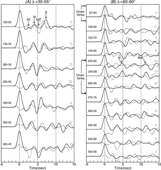
MOBC low-frequency radial (solid) and tangential (dashed) data. (A) Receiver function stacks with epicentral distances from 30° to 55°. (B) Receiver function stacks with epicentral distances from 60° to 90°. The backazimuth-epicentral distance (in degrees) for each receiver function is shown on the left. The number of traces in each stack is shown on the right.
The tangential receiver functions (Fig. 4) with along-strike backazimuths have a similar pattern to the radial component. They have a large amplitude positive peak at ∼4 s (M) followed by a negative–positive pair of phases (LVZ and B), whereas the traces from cross-strike backazimuths have much smaller amplitudes. The M-, LVZ- and B-phases lack a clear azimuthal pattern, with possible polarity reversals between 20–120° and 305–340°, but no polarity reversal associated with the traces with lowest amplitude (backazimuths from 220 to 260°). A shallow prominent conversion also occurs at ∼2 s with polarity reversals between 135–220° and 305–340°. The energy from the initial P-phase, although it may be noise, suggests either dipping interfaces or an anisotropic upper-most layer. The significant energy and polarity reversals contained on the tangential receiver functions and the azimuthal variability of the radial receiver functions suggests a shallow dipping interface (S2) striking ∼240° and a complex dipping and/or anisotropic low-velocity zone (LVZ and B) underlying an interface (M) with a large S-wave contrast and possible dip. There are several strong indicators that these features are signals produced from S-velocity contrasts beneath MOBC and not noise artefacts. For example, the individual receiver functions at a particular backazimuth are consistent with each other and the resulting stack, the features are similar across different backazimuths, and as discussed below are recorded at the other seismograph stations.
5.1 Modelling results
The crustal structure of Smith (2003) was used as a starting point for the modelling performed in this study. The model of Smith (2003) provides a good fit to the large amplitude phases for the along-strike backazimuths, but fails to reproduce the continental Moho Ps conversion for the cross-strike events (A-phase). To improve the fit of the receiver functions especially from cross-strike backazimuths and to better constrain the details of the earth structure beneath MOBC, a data inversion scheme was applied. In order to limit the number of free parameters for each inversion run, the inversion was completed in stages and the density and Vp/Vs ratio were held fixed during the entire procedure. For a reasonable range of values, the density has very little effect on the receiver functions. Density values were obtained using the equation, ρ= 0.32Vp+ 0.77 and P-wave velocities from the Spence & Asudeh (1993) refraction model. The density values are consistent with those used in gravity modelling performed along seismic lines by Rohr (2000) and Spence & Long (1995) as well as with the general Christensen & Mooney (1995) and Barton (1986) velocity–density relations. The signal-to-noise ratios (SNR) are inadequate to accurately constrain Vp/Vs, which is controlled by the signal amplitudes. The upper 5 km of crust is assumed to have a Poisson's ratio, σ, of 0.266 (Vp/Vs= 1.77), as determined by Bérubé (1989) from a microseismicity study in the QCI. The underlying layers, which are interpreted to be dominantly mafic, are assigned σ= 0.30 (Vp/Vs= 1.90), consistent with the average values for oceanic crust and basalt (Christensen & Mooney 1995). The parameter bounds chosen for the layer thickness and S-wave velocities during the inversion were based on the P-velocity structure and uncertainties from seismic refraction studies of the Queen Charlotte margin (e.g. Spence & Asudeh 1993). Separate inversions were carried out for the low-frequency receiver functions that have good SNR but poorer spatial resolution, and the high-frequency receiver functions that have poorer SNR but better spatial resolution.
5.2 Low-frequency radial receiver functions
The first inversion stage was for a 5-layer model (Fig. 5) to reproduce the main arrivals (M, LVZ, B and Mult) observed on the low-frequency receiver functions. The data were first inverted for S-wave velocity and layer thickness, in order to constrain the primary layering before including dip. A second inversion step was performed to obtain the dip angle and direction of the low-velocity zone. A further inversion then refined the layer thickness and velocities fixing the orientation of the low-velocity layer. The inversion was repeated numerous times with different parameter bounds and inversion parameters. All inversion runs with reasonable parameter bounds, that is, within the uncertainties of geological and geophysical constraints, gave an east-dipping low-velocity zone with a strike of ∼330° (±20°) and dip of 28° (±5°).
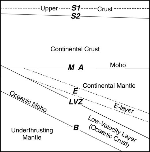
Schematic cross-section of the velocity structure used during the receiver function modelling at MOBC. Solid lines are the interfaces included in the inverse modelling of the low-frequency data and the dashed lines are the interfaces added during the forward modelling of the high-frequency data. The bold italic letters show the Ps conversions (labelled in Fig. 4) produced from the interfaces.
A shallow dipping layer in the upper crust was then added to model the azimuthal variation of the S2-phase on the radial component and the energy and polarity reversals of the S2-phase observed on the tangential component. The best fitting interface is at a depth of ∼3–4 km with an eastward dip of ∼5°. The addition of the shallow dipping layer improved the fit of the S2-phase on the low-frequency radial receiver functions for backazimuths of 120°, 220° and 260°.
Additional inversions were also performed to test for dip of the continental Moho. Moho dips of up to 15° with a strike of 300–350° were obtained with minimal changes to the misfit (<0.01). Although the inversion could not determine if there is a dipping continental Moho, forward modelling tests showed that a northeastward dip of 10° appeared to improve the fit of the cross-strike radial receiver functions (backazimuths of 220–260°). The addition of the east–northeastward dip of the Moho and shallow layer delays the arrival of the Moho conversion (A-phase) on the cross-strike radial receiver functions, improving the fit of the timing of the modelled phase.
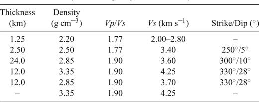
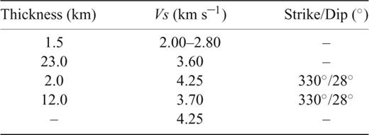
The final model (Table 1) is similar to Smith (2003), but our additional data and analysis allow the dip of the low-velocity layer to be constrained to 28° compared to the 20° dip in their model. The new model gives a fit to the data that is very good on the radial component (Fig. 6), especially for the traces from smaller epicentral distances (30–55°). The Ps conversions produced from the Moho and the upper and lower interfaces of the low-velocity zone are reproduced well on the along-strike receiver functions. The southeastern (120–135°) and cross-strike (220–260°) receiver functions have a much improved fit to the Smith (2003) model. The model Moho multiple (Mult) produces a good fit on all the waveforms, except that the predicted amplitudes are larger than observed on some of the backazimuths (120°, 135°, 285° and 300°) from closer epicentral distances. The large lateral sampling area and variations in amplitude and arrival time as a function of backazimuth and epicentral distance make it difficult to accurately model multiples phases (Cassidy 1992). The M-, LVZ- and B-phases on the observed north–northeast (355–100°) waveforms arrive 1–2 s later than predicted from the model. The poor fit of the north–northeast waveforms may result from 3-D structure, such as a northward thickening of the continental crust, which is consistent with the results of seismic refraction and reflection studies (e.g. Spence & Long 1995).
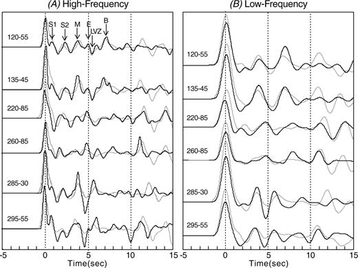
Final six-layer low-frequency S-wave velocity model for MOBC.
MOBC low-frequency radial receiver functions (black) versus final S-wave velocity model (Table 1; grey). (A) Receiver function stacks with epicentral distances from 30° to 55°. (B) Receiver function stacks with epicentral distances from 60° to 90°. The backazimuth-epicentral distance (in degrees) for each receiver function is shown on the left.
5.3 High-frequency radial receiver functions
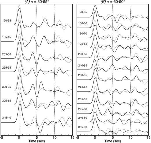
Generally, high-frequency receiver function waveforms are more susceptible to scattered energy, making them harder to model and interpret. However, for MOBC the main conversions observed on the low-frequency receiver functions, S2, M, LVZ, B and Mult are easily recognized on the most stable stacked high-frequency receiver functions (Fig. 7a). Two additional coherent phases are identified, a very shallow interface (S1) and a low amplitude negative–positive pair of arrivals (E) following the Moho conversion (M) and preceding the conversion from the modelled oceanic crust of the underthrusting slab (LVZ) (Fig. 7a). Starting with the 6-layer model determined from the low-frequency modelling, an 8-layer model was found using the RAY3D forward modelling code. A dipping low-velocity zone was added above the underthrusting slab to fit the negative–positive pair of arrivals (E). The S-wave velocity and thickness of the two thin shallow upper crustal layers were also varied to refine the fit of the S1- and S2-phases on the high-frequency radial receiver functions.
(A) MOBC high-frequency radial receiver functions (black) versus final 8-layer model (grey). (B) MOBC low-frequency radial receiver functions (black) versus final 8-layer model (grey). The backazimuth-epicentral distance (in degrees) for each receiver function is shown on the left.
The synthetic high-frequency receiver functions produced from the 8-layer model are similar to those from the 6-layer model. However, the more complex model reproduces the low-amplitude negative–positive pair of arrivals (E) observed on the southern (backazimuths of 120–260°) receiver functions (Fig. 7a). The addition of the thin low-velocity layer above the oceanic slab also enhances the correlation of the cross-strike (backazimuths of 220–260°), low-frequency, radial receiver functions (Fig. 7b). In particular, the amplitude and timing of the A-phase has an excellent fit compared to all previous models.
In order to test the necessity of the dipping low-velocity zone, synthetic receiver functions were calculated from the final velocity model without a low-velocity layer and dipping interfaces (Fig. 8a) and with a horizontal low-velocity layer (Fig. 8b). The synthetics for both cases have a very poor fit to the observed data compared to a model with a dipping low-velocity layer (Fig 8c). The large negative peak (LVZ-phase) at ∼4–6 s on the waveforms is absent from the synthetic receiver functions calculated from a velocity model without a low-velocity layer (Fig 8a). This suggests that the low-velocity layer is required by the data to fit the negative–positive pair of phases (LVZ- and B-phases). The synthetics calculated from a velocity model with a non-dipping low-velocity layer (Fig 8b) only produce a good fit to the waveforms from backazimuths of 120 to 135°. Dipping interfaces for the low-velocity layer are therefore required to reproduce the azimuthal variations of the M-, LVZ- and B-phases on the observed receiver functions. A Chi-square test was also performed to determine whether the improved fit obtained with dipping interfaces for the low-velocity layer was statistically significant. The results of the Chi-square test showed that the assumption that there is no statistical difference in the misfit between models with or without the dipping interfaces can be rejected at >95 per cent confidence.
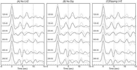
MOBC low-frequency radial receiver functions (black) versus synthetics (grey) from the final S-wave velocity model (C) compared to synthetics from an S-wave velocity model without dipping interfaces (strike/dip of all interfaces set to 0°/0°) and with (B) and without (A) a low-velocity layer (S-wave velocity of 12 km thick layer five changed from 3.70 to 4.25 km s–1).
5.4 Tangential receiver functions
The comparison of the synthetic receiver functions computed from the 8-layer structural model for MOBC to the tangential component of the receiver function data is shown in Fig. 9. The fit is poor compared to the radial component. The predicted times associated with the shallow dipping interface fit the observed timing of the phases in the first 3 s, although the predicted amplitude of the negative peak at ∼2–3 s is much smaller than observed. The timing, and for some traces the amplitude, of the arrivals produced by the Moho and oceanic slab are modelled well; however, the polarity of the predicted phases for backazimuths of 340–135° are reversed from the observed data, possibly resulting from anisotropy. Synthetic receiver functions were calculated by Bustin (2006) for models with anisotropic layers using a ray theoretical method (Frederiksen & Bostock 2000) capable of modelling dipping, anisotropic media. The modelling showed that although anisotropic structures are insufficient to explain the azimuthal variation observed on the radial receiver functions it may be required in addition to dipping interfaces to produce the pattern of polarity reversals observed on the tangential receiver functions.
MOBC low-frequency tangential receiver functions (black) versus model with a dipping oceanic slab (grey). The backazimuth-epicentral distance (in °) for each receiver function is shown on the left. The fit is poor, which may indicate the presence of anisotropy in addition to the dipping interfaces.
5.6 Sensitivity analysis
The sensitivity of the S-velocity model to changes in the model parameters was investigated by calculating the variation in the correlation misfit to perturbations in the parameters about the final model. Fig. 10 shows plots of the change in misfit versus change in individual model parameters for the crustal thickness and velocity as well as the dip and strike of the low-velocity zone. This is only a first order test since it does not deal with parameter trade-offs. The uncertainties of the model parameters were estimated from: (1) the sensitivity analysis (range of values that produce small, that is, <0.005, changes in the misfit), (2) inversion and forward modelling tests, (3) as well as from examining the complete ensemble of models and their corresponding misfits obtained during the inversions. The estimated sensitivities are: thickness ±3 km, velocity ±0.2 km s–1, strike ±30° and dip ±5°. The sensitivity of the model to density and the ratio of P- to S-velocities were also tested. The analysis showed that varying these parameters within reasonable ranges (0.25–0.35 for σ and ±0.2 g cm–3 for ρ) only resulted in minor increases in the misfit (<0.005).
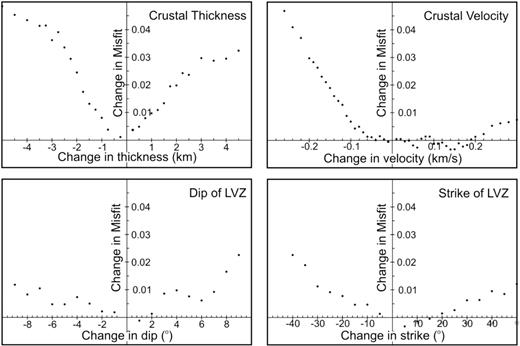
Plots of the change in misfit versus change in model parameters for the crustal thickness and velocity, and the strike and dip of the low-velocity zone.
The timing of a converted phase on a receiver function is dependent on the product of the depth and S-wave velocity, resulting in a trade-off between the two parameters. With large bounds on the parameters, the inversion can converge on a solution that is geologically unreasonable. This problem is enhanced for inversions of noisy and/or limited data sets. The non-uniqueness of the receiver function inversion can be minimized by using a priori information. During this study a priori constraints provided by seismic refraction studies were required to bound the thickness and velocities of the model. Additional limitations of the inversion procedure include assuming interface planarity and perfect elasticity during the forward modelling. The assumption of planar interfaces may cause difficulties in accurately modelling multiple phases, which sample a relatively large lateral area (Cassidy 1992). Lateral variations in the Earth structure need to be consider in order to model reverberations, particularly from deep dipping interfaces.
The depth–velocity trade-off was examined for the low-velocity layer in the model. Good fits to the data (<0.005 change in misfit) were obtained for a layer with a minimum thickness of 7 km with a corresponding velocity of 3.5 km s–1 and a maximum thickness of 15 km with a velocity of 4.0 km s–1.
6 OTHER SEISMIC STATIONS
6.1 DIB seismograph and results
A model for the crustal structure beneath DIB was found by forward modelling the low-frequency receiver functions, using the velocity structure determined at MOBC as a starting model, including a dipping low-velocity zone. However, the dipping structure could not be constrained, due to the limited data set. The high-frequency receiver functions were not useful due to high noise levels.
The S-wave velocity model for DIB was constructed by determining the depths of the Moho interface and oceanic slab given their orientation and distance from the MOBC station. Small changes to the velocity structure were tested to improve the fit of the observed and calculated radial receiver functions. The final model is shown in Table 2 and the resulting fit to the radial component data are shown in Fig. 11. Only the stacks with greater than five traces were included in the modelling, since the remaining stacks did not possess coherent phases and were inconsistent with the individual waveforms. The synthetic receiver functions contain a prominent positive conversion at ∼3–4 s followed by a negative peak at ∼4–5 s. These phases, which are interpreted to be produced by the Moho interface and the top of the oceanic slab, correlate well with the observed waveforms. An additional shallow phase (∼1.5–2 s) is observed at backazimuths of 120° and 230°, which was not modelled. The synthetic receiver functions contain a multiple phase at ∼10–12 s associated with the continental Moho. The multiple arrives ∼1 s earlier than predicted by the model for the observed receiver function at a backazimuth of 230° and epicentral distance of 85° and is absent from the data for smaller epicentral distances. More data are needed to determine the cause of this discrepancy.
Final S-wave velocity model for DIB.

Low-frequency radial receiver functions recorded at DIB (black) versus best-fitting model (Table 2; grey). The backazimuth-epicentral distance (in degrees) for each receiver function is shown on the left. The number of traces in each stack is shown on the right.
6.2 Temporary seismic stations
Limited forward modelling analysis was performed on the receiver functions calculated at the temporary seismic stations. The data are of poorer quality but led to several important conclusions. The QURY seismograph, which was located at approximately the same distance from the QCF as the MOBC permanent station, produced very similar receiver functions over a number of backazimuths. The main conversions and multiples at MOBC have comparable amplitude and timing in the QURY traces.
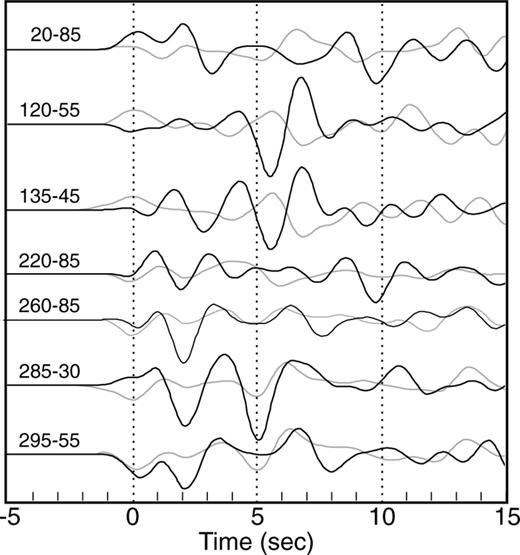
The waveforms from a backazimuth of 295° and epicentral distance of 30–55° recorded at every site are shown in Fig. 12. The LVZ- and B-phases produced by the low-velocity layer and observed at MOBC and DIB are also present at the temporary sites. These phases shallow westward across the QCI, confirming the eastward dip interpreted at MOBC. The M-phase from the continental Moho is also present within a similar time window for the easterly sites. The Moho conversion disappears from DAWS, which is expected since this site is very close to the boundary between the modelled base of the continental crust and the top of underthrust oceanic crust. S-wave velocity structure beneath the four temporary stations was determined by calculating the depths of the interfaces given the basic structure interpreted at MOBC. Although the dipping structure at these stations could not be constrained due to the limited amount of data, the final models (Table 3) produce excellent fits. These observations indicate that the velocity structure observed at MOBC occurs regionally and provides the first evidence that the dipping low-velocity zone modelled at MOBC is not a local feature.
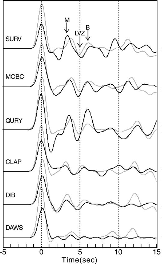
Low-frequency radial receiver functions from a backazimuth of 295° and epicentral distance of 30–55° recorded at all stations (black) versus best-fitting models (grey). The station names are shown on the left.
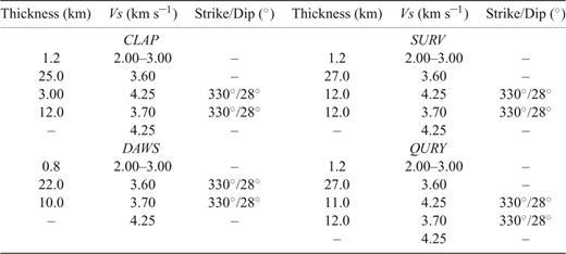
Final S-wave velocity models for the temporary stations.
7 DISCUSSION
The final model for the S-wave velocity structure beneath the QCI determined from the teleseismic receiver function analysis (Fig. 13) has a thin continental crust that thickens landward, underlain by a landward dipping low-velocity zone interpreted to be underthrusting oceanic crust. The depth of the underthrusting slab offshore beneath the terrace and QCF is inferred from the reflection seismic section across the Queen Charlotte Terrace and the results from seismic refraction and gravity modelling (e.g. Davis & Seeman 1981; Horn 1984; Spence & Asudeh 1993; Spence & Long 1995). As discussed above, certain features of the model are required by the timing, polarity, and amplitude of the converted phases, while other features are less constrained. The main characteristics of the model and their implications for the tectonic structure in the Queen Charlotte region are discussed below.
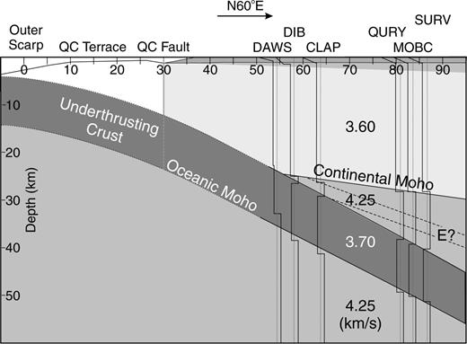
Model S-wave velocity structure beneath the Queen Charlotte Islands determined from the teleseismic receiver function analysis. Velocity profiles modelled at each station are shown. Black dashed lines show the location of the modelled E-layer. Thick grey vertical line shows the location of the Queen Charlotte Fault with the dashed portion representing its possible extent into the underthrusting crust. S-wave velocities are in km s–1.
7.1 Geometry of the underthrusting slab
The low-velocity zone modelled beneath the QCI is necessary to fit the negative–positive pair of arrivals (LVZ and B) observed on the receiver functions recorded at each of the permanent and temporary stations across the Islands. The azimuthal variability on the radial component and the significant tangential energy requires that the low-velocity zone dips eastward and that it may be anisotropic. The eastward deepening of the low-velocity layer across the QCI modelled by DIB and the temporary stations provides further strong evidence that the low-velocity layer is dipping eastward. The modelling at MOBC has shown that a strike of 330°± 30° and dip of 28°± 5° for the low-velocity layer provides a good fit to the data.
The depth, orientation and S-wave velocity of the low-velocity layer are consistent with the crust of an oceanic plate underthrusting beneath the QCI. Seismic studies and receiver function analysis at many subduction zones (e.g. Alaska, Andes, Cascadia and Japan) have revealed the presence of a thin (≤10 km thick) dipping low-velocity layer (10–20 per cnet S-velocity contrast), which is generally interpreted as subducting oceanic crust that has not transformed to eclogite (Peacock & Wang 1999 and references therein; Rondenay 2001 and references therein; Hacker 2003). The thickness of the underthrusting crust beneath the QCI was modelled as 10 km with an uncertainty range from 6 to 13 km. A value of ∼7 km would correspond to the thickness of the oceanic crust beneath the Queen Charlotte Terrace modelled from seismic refraction studies. A greater thickness could result from crustal thickening (e.g. tectonic shortening prior to or during underthrusting) or the underthrusting of abnormally thick oceanic crust (e.g. oceanic plateau).
7.2 Crustal thickness and Moho dip
The teleseismic receiver function analysis revealed a shallow continental Moho beneath the QCI, with depths thickening landward from ∼25 km in the west to 28 km in the east. These depths are in excellent agreement with the Spence & Asudeh (1993) refraction model average of ∼27 km. This thin continental crust does not support a tectonic model of the plate convergence being taken up by crustal thickening unless the initial crust was very thin. The modelling of MOBC data revealed a possible east–northeastward dip of the continental Moho. A dip of 10° provides the best fit to the receiver function data but its addition does not reduce the misfit enough to be confident that it is required by the data. Forward modelling at DIB and the temporary stations could not constrain the 2-D structure at individual sites. However, the continental Moho modelled to reproduce the M-phase at the profile of sites implies an east–northeastward dip of ∼10°, similar to that suggested by the inverse modelling at MOBC. This dip results in ∼5 km of shallowing of the Moho westwards towards the QCF. Assuming that the Moho was originally horizontal and that the crust was of constant thickness this result is in agreement with the westward rise in elevation across the Islands, possibly resulting from the upward flexure of the North America Plate due to the initiation of underthrusting (Hyndman & Hamilton 1993; Prims 1997).
7.3 E-layer
The 8-layer model obtained beneath MOBC from the high-frequency receiver functions contains a second dipping low-velocity zone beneath the continental crust, 3 km above the underthrusting slab and with similar orientation. Such a layer could correspond to the reflective low-velocity E-layer, which has been observed at the Cascadia subduction zone. In a teleseismic receiver function analysis, Cassidy & Ellis (1993) observed a prominent low-velocity zone, which they interpreted to correlate with the E-reflection zone in LITHOPROBE reflection data beneath Vancouver Island (e.g. Yorath 1985; Clowes 1987). The E-layer was modelled to lie several kilometres above the subducting plate with similar orientation and a shallower dip of ∼15° to the north–northeast, and to have a thickness of 5–10 km. These results are consistent with the thin low-velocity zone modelled by the high-frequency receiver functions at MOBC. The E-zone has been interpreted to be related to intensely sheared sediments that trap fluids released during subduction or dipping lenses filled with fluids from dehydration reactions within the subducting oceanic slab (Hyndman 1988; Nedimović 2003 and references therein). However, the location and relationship of the Cascadia E-layer with respect to the subducting Juan de Fuca plate is still uncertain. In the interpretation of a recent passive seismic experiment, Nicholson (2005) proposed that the dipping low-velocity zone observed on teleseismic studies is the subducting oceanic plate and the reflective E-layer is located within the slab.
8 CONCLUSIONS
Strong evidence supporting a plate model with an underthrusting Pacific slab beneath the QCI has been provided by analyses and modelling of teleseismic receiver functions at a profile of stations across the QCI. The receiver functions were calculated using time-domain iterative deconvolution on the three-component broad-band data recorded at the permanent seismic stations MOBC and DIB as well as at four temporary stations. The interpreted crustal structure beneath the central QCI contains a ∼10 km thick low-velocity slab dipping eastward at 28°. The interpreted underthrusting slab, which may be anisotropic, is located between 28 and 39 km depth beneath a thin (average 28 km) westward shallowing (10°) continental crust. Although the model is quite complex, the main parameters of an underthrusting low-velocity slab are well constrained. An eastward dipping thin E-type low-velocity zone may also be present in the mantle overlying the underthrusting slab. The results support the interpretation that the component of Pacific–North America convergence along the margin of the QCI for the past ∼5 Myr has been accommodated at least in part by underthrusting of the Pacific Plate. The receiver functions also indicate that the dipping slab extends at least 50 km landward beneath the QCI, that is, a significant part of the estimated 80–160 km component of convergence.
REFERENCES
