


Summary
A regional model of the 3-D variation in seismic P-wave velocity structure in the crust of NW Europe has been compiled from wide-angle reflection/refraction profiles. Along each 2-D profile a velocity–depth function has been digitised at 5 km intervals. These 1-D velocity functions were mapped into three dimensions using ordinary kriging with weights determined to minimise the difference between digitised and interpolated values. An analysis of variograms of the digitised data suggested a radial isotropic weighting scheme was most appropriate. Horizontal dimensions of the model cells are optimised at 40 × 40 km and the vertical dimension at 1 km. The resulting model provides a higher resolution image of the 3-D variation in seismic velocity structure of the UK, Ireland and surrounding areas than existing models. The construction of the model through kriging allows the uncertainty in the velocity structure to be assessed. This uncertainty indicates the high density of data required to confidently interpolate the crustal velocity structure, and shows that for this region the velocity is poorly constrained for large areas away from the input data.
1 INTRODUCTION
Models of the seismic velocity structure of the continental crust play an important role in seismology as the starting point for a variety of types of study. They can be used for improved location of earthquakes, thus assisting in defining and mitigating seismic hazards. Global models of crustal velocity structure (e.g. Bassin 2000) may be used in the application of traveltime corrections to teleseismic arrivals, facilitating investigation of the interior of the earth. In conjunction with earthquake data, models may be used as the starting point for crustal tomography, which in turn adds new information to the model, refining it and improving its resolution. In addition to applications in seismology, crustal models define variations in physical properties, which have applications in modelling of tectonic processes and the evolution of the continental lithosphere.
Deep seismic refraction profiles have been acquired around the world since the 1950s, providing snapshots of the crustal structure beneath the survey areas. As the quantity of data has grown numerous authors have brought together the individual surveys into global or regional compilations and used the data to map out the thickness and structure of the crust [at least 38 compilations of crustal structure data were published before 1998 (Mooney 2002)]. With ever increasing quantity and quality of individual surveys, there has been a continual improvement in the detail of these models. However, the global coverage of seismic data is still quite sparse and data are very irregularly distributed, limiting the global models to relatively coarse grid dimensions [e.g. 2° for CRUST2.0 (Bassin 2000)]. Regional studies in densely surveyed areas allow significant refinement of the models and thus much greater detail may be included. As a result of extensive scientific research in conjunction with hydrocarbon exploration, NW Europe is unique in having substantial coverage by deep seismic refraction profiles over such an extensive area. In this contribution the available data in NW Europe have been compiled and digitized, building on an earlier compilation (Clegg & England 2003) for the region.
As well as controlled source profiling, a number of natural source techniques provide information on the thickness and structure of the crust, such as delay time analysis, receiver functions and tomography. However, controlled source wide-angle reflection/refraction seismic profiling (hereafter referred to as wide-angle seismic data) offers a number of distinct advantages as a starting point for building models of the crustal velocity structure. Primarily, through modelling, wide-angle seismic data recovers true, or interval, velocity and depth to major interfaces within determinable uncertainties. Little or no a priori information is required. In contrast, normal-incidence reflection, tomographic, delay time and receiver function methods suffer from the coupled uncertainty between velocity and depth to interfaces, unless a priori constraints are available. Most wide-angle seismic reflection experiments are conducted with particular targets in mind and hence receiver and source locations are usually planned for optimum coverage of the subsurface. In contrast, passive experiments are restricted by the range of backazimuths of those events occurring during the recording period. However, passive techniques may give a better indication of the range of anisotropy present while most refraction experiments have, to date, been 2-D and hence their spatial or azimuthal coverage is restricted. This contribution describes the construction of a 3-D model of crustal P-wave velocity structure for the UK, Ireland and surrounding seas, based on interpolation of 2-D wide-angle seismic profiles by ordinary kriging. The complete velocity model can be obtained as an ascii file from
2 THE DATABASE
The model is built from a database that provides the input for three surfaces (topography/bathymetry, top basement and Moho) and two layers (sediments and crystalline basement). At the core of the model is a database of digitized wide-angle seismic profiles that provide the input data for the velocity of the crystalline basement layer and the Moho depth. The locations of the profiles included in the database are shown in Fig. 1 and a complete listing of the profiles and the primary source of the data is listed in the Appendix. Each profile was sampled at 5 km intervals to provide a suite of 1-D velocity–depth functions and Moho depth information. Velocity values were initially recorded at the exact depth of nodes or boundaries in the published model; then, after checking for errors, were resampled to 100 m depth intervals using linear interpolation.
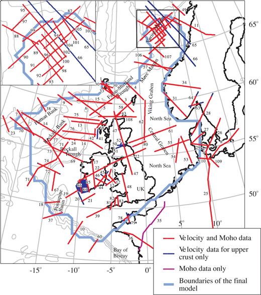
Map showing the locations of wide-angle seismic data entered into the database (Numbers on seismic profiles refer to the listing in the Appendix). Coastlines and 1 km bathymetry contours are marked on this and all subsequent maps.
Uncertainties in the velocities and Moho depths have been assigned to the wide-angle seismic data and have been included in the database. Where available, published uncertainties have been used, but it is rare for a comprehensive review of uncertainties to be included in most published work. Consequently, experience with modelling wide-angle seismic data and estimates based on comparable published work have been used as a guide in making qualitative uncertainty estimates. Experiments were considered comparable when they used similar source and receiver coverage and modelling methods. These two factors were the primary considerations in assessing uncertainties. Models constructed using ray tracing methods or methods in which the velocity structure is determined by traveltime tomography with the Moho included as a floating reflector (e.g. FAST, Zelt and Barton 1998) were considered ‘good’. Modelling using time term methods, T2–X2 and other miscellaneous methods were considered ‘poor’. Simple fitting of constant velocity layers on the basis of gradient and intercept time of arrivals on record sections was considered ‘very poor’. This qualitative assessment included whether the modelling was 1-D or 2-D, with 1-D models being considered significantly poorer than 2-D models. Methods based on inverse, rather than forward, modelling were considered superior, although less emphasis was placed on this than the general modelling method. The density of data coverage (i.e. spacing of receivers and shots) and whether the survey had reversed coverage were considered almost as important to the velocity uncertainty as the modelling method. The data coverage was generally assessed through published ray path diagrams. Inspection of ray path coverage was considered particularly significant when assessing uncertainty in Moho depth as is it rare for a survey to have PmP reflections along the full length of the profile. Large sections of the Moho are often unsampled in even the best-designed experiments with good data recovery (e.g. Klingelhöfer 2005). Additionally, the use of gravity modelling was considered to improve the uncertainty in the depth to the Moho, particularly in regions poorly constrained by PmP reflections, but to be very much secondary to the seismic modelling method and data coverage. The use of amplitude information was considered to significantly reduce uncertainties in velocities by better defining gradients in the models. The quality of the data in terms of signal-to-noise ratio was also examined, although not considered as significant. Within the published wide-angle seismic models coincident normal incidence reflection surveys have been used in a number of ways: to construct a starting model; to constrain the sediment geometries and velocity structure; directly as additional data in the modelling; and as an independent source of data to assess the final model. When used in either the first or second approach, the normal incidence data is considered to help produce a more accurate final model, but to have little effect on the constraint/uncertainty of that model. In the third approach the data is considered during the assessment of data coverage. If used only to assess the final model the data has no effect on the constraints on velocity.
Uncertainties have generally been assigned as percentages of the velocity values and as absolute uncertainty, in kilometres, for the Moho depths. The two most common modelling methods are ray tracing and time-term analysis. Typical errors assigned to a ray traced model with good data coverage (e.g. ocean bottom recorders every 30–60 km and dense coverage of airgun shots) and consideration of amplitude data would be ∼3 per cent (approximately equivalent to ±0.2 km s−1) for the upper crust and ±5 per cent (∼±0.35 km s−1) at the base of the crust. The models in which time-term analysis has been used are generally older than the ray traced models and so have poorer data coverage and amplitude data is not used. As a result such models are typically assigned errors of ±7 per cent (approximately equivalent to ±0.3 km s−1) for the upper crust increasing to ±10 per cent (∼±0.6 km s−1) at the base of the crust. The depths to mid-crustal interfaces were not assigned uncertainties as this information is largely redundant. In the case of first order discontinuities, the uncertainty on mid-crustal interfaces is related to the velocity step across the interface. Interfaces associated with large velocity discontinuities are generally well constrained. Only those interfaces associated with small velocity steps (or highly uncertain velocities) are poorly constrained. Therefore, where interfaces are poorly constrained the velocity step across the interface is generally much smaller than the uncertainties in the velocity values on either side. As a result the discontinuity is largely masked by the velocity uncertainties and the uncertainty on its depth becomes relatively irrelevant. A full list of the assigned uncertainties for each model is given in the Appendix.
At locations where published 2-D models intersect there is often a small difference in the interpreted crustal structure, both in terms of the Moho depth and the velocity structure. In such cases the data were recorded in the database with their original, published values. If necessary the uncertainties assigned to the data were increased to incorporate the different values at the intersections. In building the velocity model, described below, any such differences were accommodated by averaging the values at the intersections.
Where the sedimentary layer is present, a 1-D profile of increasing velocity with depth was used to define the velocity structure. This velocity–depth function was derived using the interval velocities calculated from stacking (rms) velocities taken from the reflection profiles listed in Table 1. These data were chosen to cover each of the major sedimentary basins in the region. The velocity data were converted to a mean velocity–depth profile by calculating a power regression curve through the median value of velocities (binned into 0.5 km depth intervals) (Fig. 2). An estimate of the uncertainties associated with the velocity of the sediments was acquired by fitting similar regression curves through the 5th and 95th percentiles of the binned data (Fig. 2). The equations that define the minimum, best-fitting and maximum velocity values are: 5th percentile v= 2.1648z0.2929; median v= 2.909z0.2255; 95th percentile v= 4.8018z0.0584; where v is velocity (km s−1) and z is the depth below the surface/sea bed (km).
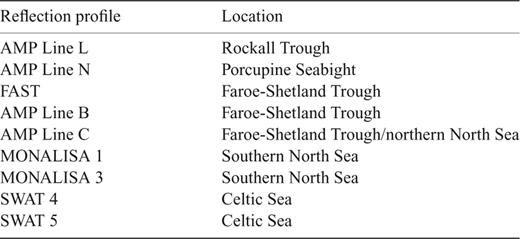
Seismic reflection profiles used as sources of data on P-wave velocity variation with depth in the sedimentary basins.
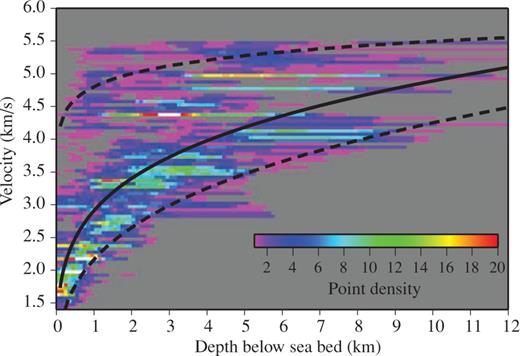
Interval velocities plotted against depth from nine regional seismic profiles from around the UK (Table 1) used to derive the mean velocity–depth function used in the sedimentary layer—solid black line. Broken lines are the minimum and maximum velocity–depth functions.
The top surface of the model is defined by the topography and bathymetry. The data used in the model were extracted from the Smith & Sandwell (1997) bathymetry and GTOPO30 topography.
The interface between the sediments and crystalline crust was compiled from a number of data sources. For much of the model the NGDC map of ‘Sediment Thickness in the World's Oceans and Marginal Seas’ (National Geophysical Data Center 2004) defines the surface. This map was not used in the North Sea as it follows the base of the Mesozoic syn-rift sediments and does not include the significant thickness of pre-rift Permian sediments in the region. In the North Sea top basement picks in the BIRPS reflection data (Klemperer and Hobbs 1991) were converted to depth using an empirically derived velocity function based on a conversion of stacking (rms) to interval velocities and high-resolution wide-angle seismic data. These profiles were then extrapolated using the tensioned minimum curvature algorithm of Smith & Wessel (1990). For onshore Britain a digital version of the Variscan unconformity was provided by the British Geological Survey and was used to define the base of the sediments. These data are published in Whittaker (1985). In regions not covered by the data sets described above, the base of the sediments was taken from a 1° resolution, global map of sediment thickness (Laske & Masters 1997). The only exceptions are Scotland and Ireland where the sediment thicknesses were set to zero as the 1° resolution of the global data results in artificial sediment thickness in regions of short-wavelength topographic change.
3 Construction of the velocity model
The model is defined using Cartesian coordinates, with distances measured in kilometres, based on a Transverse Mercator projection centred at 3.4° west, 57.15° north. The velocity structure of the crystalline crust was constructed by interpolation of the digitised wide-angle seismic data assuming that the data were a randomly distributed set of points. This assumption fails in the direction of the profiles but is valid between profiles in the areas in which the velocity is to be interpolated, since the majority are not arranged systematically. The interpolation method was 3-D ordinary kriging using the Deutsch and Journal (1998) code KT3D. The Moho surface was also built primarily through ordinary kriging using KT3D. However, the regions around the Porcupine Bank and Biscay Margin were adjusted after gravity modelling, discussed below.
3.1 Ordinary kriging
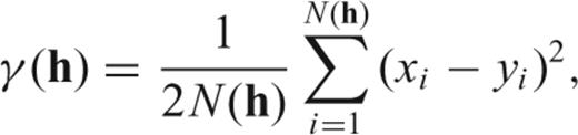
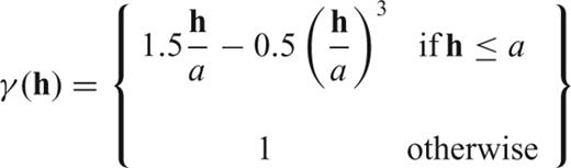
Kriging is an interpolation technique that utilizes knowledge of the spatial continuity of a variable to estimate its value away from data points. Kriging assumes that the spatial autocorrelation of the variable (in this case velocity or Moho depth) is known in the form of the semi-variogram or covariance, and uses this to weight data points and estimate the value of the variable away from the known sample locations. This use of the statistical model to produce weights for the interpolation makes kriging a superior technique compared to traditional methods, such as inverse distance interpolation, which use a weighting function that may not be appropriate for the data.
The spatial continuity of the variable is described by the variogram model. This is determined through analysis (variography) of experimental variograms constructed from the sample data.
3.2 Variography
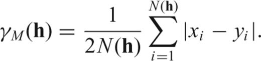
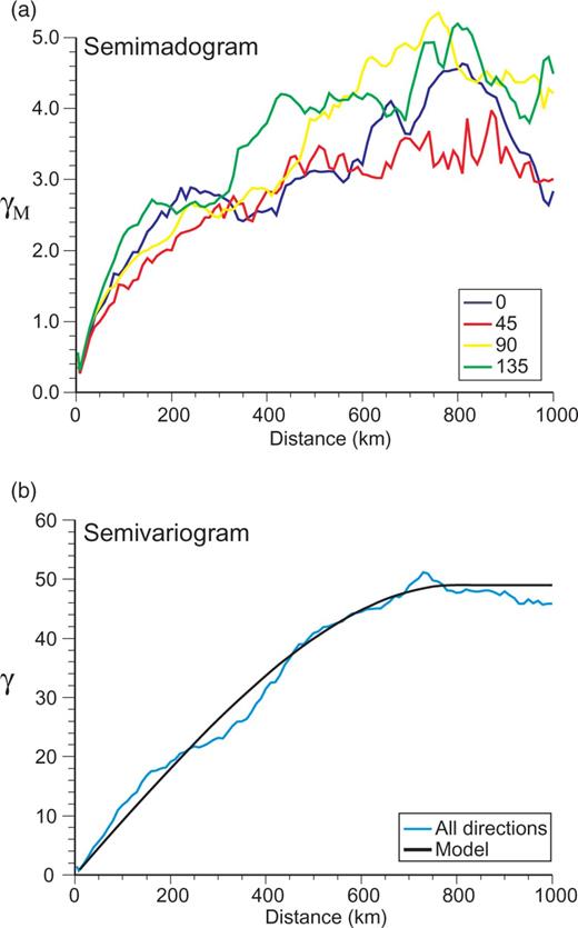
Experimental and model variograms for the Moho depth data. In each case spatial variability is plotted against lag (the distance between samples). Range is the maximum lag over which the data shows spatial continuity. The sill is the plateau associated with the maximum variation in the correlated data. (a) Semi-madograms for the Moho data, calculated only for data separated along the azimuth given in the legend (±22.5°). (b) Experimental and model semi-variograms for the Moho data.
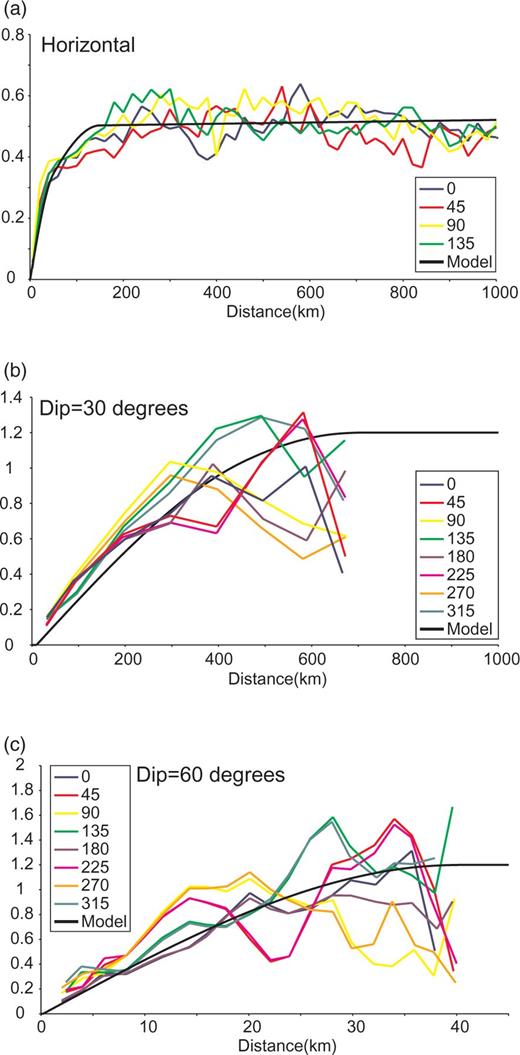
Experimental and model variograms for the crystalline crust velocity data. In each case spatial variability is plotted against lag for data separated along the azimuth given in the legend. (a) Semi-variograms for the crustal velocity derived from a search in the horizontal plane through the model space. Black line is the best-fitting curve to the experimental data. (b) Semi-variograms for the crustal velocity derived from a search in a plane dipping at 30° through the model space. (c) Semi-variograms for the crustal velocity derived from a search in a plane dipping at 60° through the model space.
The experimental variograms were inspected to assess anisotropy, range, near origin behaviour and structure at intermediate lags.
3.2.1 Anisotropy
For both the Moho and velocity data sets the experimental variograms show evidence for anisotropy. In the Moho data there is zonal anisotropy, that is, a direction dependent sill (the maximum value to which the variogram tends at large lags) but constant range (the distance at which the difference from the sill is negligible), with a minimum sill, that is, minimum variability, in a NE or NNE direction (Fig. 3a). Such a trend is likely to be inherited from the relatively high sampling of the continental margin between Hatton Bank and the Vøring Margin. Along this margin the topography and Moho depths show a rapid change in a NW direction associated with the transition from continent to ocean, but far greater continuity in the NE direction, parallel to the margin (Fig. 1). It is also possible that the NE–NNE structural trend generated during the Caledonian Orogeny has some residual signature affecting the Moho data away from the continental margin. However, since a visual inspection of the data suggests that the strong anisotropy is restricted to the northwest European continental margin, the risk of overinterpreting and introducing erroneous structure into the interpolated Moho surface was considered too high to include anisotropy in the model.
The velocity data show unquestionable dip-dependent zonal and geometric anisotropy, that is, dip-dependent sill and range, with the horizontal variograms exhibiting greater ranges and lower sills than the dipping variograms (cf. Figs 4a–c). This is consistent with what is known of the crustal velocity structure from 2-D models. A vertical profile through the crust may well show increasing velocity from 5 to 7 km s−1 over a few tens of kilometres depth, whereas the horizontal variation may well be less than 1 km s−1 along a 2-D profile several hundred kilometres in length. Therefore, the horizontal variation is expected to be both smaller in magnitude and spatially less rapidly changing than the vertical variation. There is no clear evidence for azimuth-dependent anisotropy. Therefore, the model variogram was constructed to reproduce the dip-dependent zonal and geometric anisotropy, but to be azimuthally isotropic.
3.2.2 Sill and range
The experimental semi-variogram for the Moho data shows a well-developed sill with a range of approximately 800 km (Fig. 3b). For the velocity data the horizontal variograms show a well-developed sill, at ∼0.5 km2 s−4, beyond a range of approximately 150 km. The sill for the dipping variograms is not well developed, but is higher than 0.5 km2 s−4. The best-fitting curve to the dipping variograms suggests a model with a vertical range of 35 km and sill of 1.2 km2 s−4 (Figs 4a–c).
3.2.3 Near-origin behaviour
3.2.4 Structure at intermediate lags
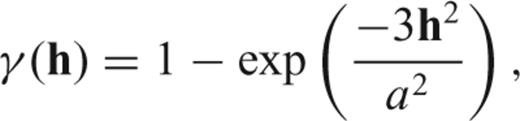
The models are broadly similar in structure at intermediate lags, differing only in the rate of change. As the Moho experimental semi-variogram (Fig. 3b) shows reasonably linear behaviour at the intermediate lags, the spherical model was preferred to the exponential model. For the velocities, the dipping variograms show reasonably smooth variation at intermediate lags. However, the horizontal variograms have a distinct change in gradient at a lag of approximately 50 km. This gradient change is reproduced by adding a second horizontal structure with a short range to cause the initial rapid increase, but which keeps the horizontal range at 150 km.
The final variogram structure chosen to model the Moho data was a single, isotropic spherical structure with a range of 800 km and sill of 49 km2 (Fig. 3b). The velocity variogram model consists of three structures: A spherical structure with a 50 km horizontal range, 35 km vertical range and 0.2 km2 s−4 sill; a spherical structure with a 150 km horizontal range, 35 km vertical range and 0.3 km2 s−4 sill; and a further spherical structure with infinite horizontal range, 35 km vertical range and 0.7 km2 s−4 sill (Fig. 4).
3.3 Dimensions of the model elements
To determine the optimum spatial dimensions of the model elements the Moho data were interpolated onto a range of grids. Investigation of the model dimension was based on the Moho data, rather than the velocity data, in order to save computational time. Given the similarity between the Moho and velocity distributions (Fig. 1), and that velocity data were interpolated with very little weight allocated to data at different depths, using 2-D data instead of 3-D data has very little impact on the evaluation of model parameters. The cell size that produced the optimum balance between reproducing details in the data and minimizing contouring artefacts (such as bulls-eye features around data points) was found to be 40 km. The vertical element size was set to reflect the balance between the desire to have fine spacing to reproduce the vertical variation seen in the input data and the need to have coarser spacing to allow for the poorer resolution of the velocity structure in the lower crust (Section 2). The Moho depth uncertainties, which have an average of approximately ±2 km, give an indication of the depth resolution in the lower crust. However, given that the resolution in the upper crust is significantly greater and that lower crustal velocity gradients are generally small, a vertical element dimension of 1 km was considered the most appropriate for the crustal layer as a whole. Prior to interpolation the data were declustered by calculating the mean value and location of data within each model cell.
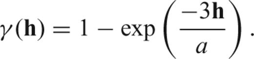
The search parameters used in the final model required a minimum of 25 and maximum of 64 data points, with the maximum per octant of 8. The search radius was set to 800 km, allowing Moho depths to be estimated at all constrained locations. The interpolated Moho depths are shown in Fig. 5a. The region encompassing the Porcupine Basin and Biscay margin has substantial bathymetric relief which is mirrored in the Moho structure imaged in the 2-D seismic profiles in the database. However, the data distribution is unfortunate in that only one profile fully samples the change from abyssal plain to continental shelf (Fig. 1). The distribution of data results in interpolated Moho depths that vary over a wider region than does the bathymetry and only weakly capture the structure of the Porcupine Basin (Fig. 5a). The velocity and Moho structure of an earlier iteration of the crustal model presented here were verified by converting the velocities to density and performing 3-D gravity modelling (Kelly 2006). The results of this modelling indicated that Moho in this region must echo the bathymetric change more closely than the interpolated data. Therefore, in producing the crustal model the Moho depths along the Biscay Margin and under the Porcupine Basin have been replaced by the depths derived from this gravity model (Fig. 6a). The interpolated Moho depths show very high uncertainties under continental Europe and Scandinavia (Fig. 5b); therefore, these areas were removed when defining the model boundaries (see Fig. 1 for model extent).
(a) Interpolated surface representing the Moho and (b) uncertainty in Moho depth. Final Moho shown in Fig. 6. Coastlines, 1 km bathymetry contours and lines of longitude and latitude are shown in white.

Surfaces used to build the velocity model. Coastlines, 1 km bathymetry contours and lines of longitude and latitude are shown in white, labels and contours indicate surface depth. (a) Moho depth, with the interpolated surface edited along the southwest continental margin after gravity modelling. (b) Basement depth, compiled from data on sediment thicknesses as outlined in the text.
An 800 km range was also used for the velocity data, ensuring that all cells within the model would be assigned a Moho depth and velocity. The kriged velocity data were combined with the sediment velocity estimates, with the layer thicknesses defined using the final Moho (Fig. 6a) and filtered versions of the topography and base-sediment surfaces (Fig 6b). The interface between the sediment and crystalline layers in general falls within one of the model cells (rather than falling exactly at the cell boundary). Therefore, to reproduce the velocity structure as accurately as possible, the cell containing the base–sediment interface is assigned a weighted average of the sediment and crystalline crust velocities. The weighting is controlled by the fraction of the cell containing sediment and the fraction containing crystalline crust.
To obtain uncertainty in the velocity of each model cell and the Moho depth, the uncertainties in the database were combined with the kriging uncertainties using the law of propagation of errors. Two assumptions were made in doing this. First, the uncertainty associated with the input data conforms to a Gaussian distribution. Second, the database uncertainties are equal to twice the standard deviation in the data. These assumptions are supported by an analysis of uncertainties from modelling the MONA LISA wide-angle seismic profile crossing the Southern North Sea (Kelly 2006). The Moho uncertainties are shown in Fig. 5 and the velocity uncertainties are shown alongside depth slices through the final model in Fig. 7 and Supplementary figures.
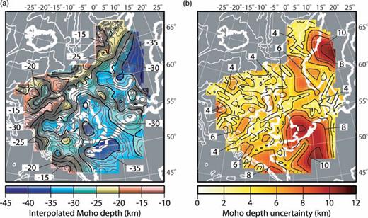
Example depth slice from the final crustal velocity model. The slice is for the cells 12–13 km below sea level. Pale grey regions are outside the model area, dark grey elements are below the Moho and therefore do not contain velocity data. Velocity contours are drawn in black at 0.25 km s–1 intervals, for velocities greater than 5.5 km s–1. Uncertainty contours are drawn in black at 0.5 km s–1 intervals.
4 Principal features of the model
The variogram model of the velocity data has a relatively short range compared to the profile spacing and this is reflected in the plots of uncertainty in velocity (Fig. 7 and Supplementary figures). As a result of the short variogram range the velocity constraint diminishes rapidly away from the data points, resulting in uncertainty maps that, once below the sediment layers clearly mimic the data distribution. Consequently, for much of the model space the calculated velocities represent a poorly constrained best estimate. The uncertainty maps also indicate the density of data required for this method of model construction to produce a well-constrained model for the whole region.
For the top few kilometres, the model shows significant lateral velocity variation associated with the sedimentary basins (Supplementary Fig. S1). By 6–7 km depth much of the model has standard upper-crustal velocities (∼6 km s–1), but in the deeper parts of the basins substantial lateral variations are maintained to approximately 10 km depth. At depths greater than 10 km the model represents the lower crust in the west and northwest, near the continental margin (Fig. 7 and Supplementary Fig. S2). As a result the velocities are higher in these areas and the model shows a notable lateral velocity gradient. At greater depths the lower crust on the northwest side of the North Sea Central Graben shows higher velocities than the southeast. Elevated velocities are also seen under Ireland and particularly the Irish Sea (Supplementary Fig. S4), a region of possible magmatic underplating (Al-Kindi 2003; Shaw Champion 2006; Tomlinson 2006).
The largest lateral variations in the velocity structure in the model are associated with the sedimentary basins (Fig. 1 and Supplementary figures). This is also shown by the mean crustal velocity (Fig. 8a). However, removing the sediments from the mean velocity calculation (Fig. 8b) illustrates that there are also variations in the velocity structure of the crystalline crust. Most notable are the higher average velocities recorded in regions where magmatic underplating is postulated to have occurred, especially along the Hatton Bank and Vøring Margin ocean–continent transitions. The median, mean and standard deviation of the crustal velocities are 6.14, 6.09 and 0.34, respectively, when including the sediment, and 6.36, 6.36 and 0.12 when using the crystalline crust only.
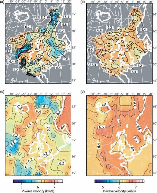
Mean crustal velocity for the new model and CRUST2.0, the most widely used existing model. (a) The mean velocity of the new model for the entire crust including sediments. (b) The mean velocity of the new model for the crystalline crust only. (c) The mean velocity of the CRUST 2.0 model for the crust including sediments (after Bassin 2000). (d) The mean velocity of the CRUST 2.0 model for the crystalline crust only (after Bassin 2000).
5 COMPARISONS WITH EXISTING MODELS
The most widely used crustal velocity model is the CRUST2.0 global 2° model of Bassin (2000). To assist the comparison between the model presented here and the CRUST2.0 model, the average velocity structure of the CRUST 2.0 model is shown in Fig. 8. The median, mean and standard deviation in crustal velocities of the CRUST2.0 model in the same region as the new model are 6.26, 6.24 and 0.21, respectively, including sediment, or 6.56, 6.50 and 0.11 excluding the sediment. These values are notably higher than in the new model. The main areas producing these differences between the two models are the sedimentary basins and shallow marine areas around Britain and Ireland (Fig. 8). The significant refinement in cell size for the new model results in far greater detail for the marine sedimentary basins; for example the Rockall and Porcupine basins are only poorly resolved in the CRUST2.0 model, but are well defined, and have lower mean velocities, in the new model. However, most of the difference comes from the shallow marine areas around Britain and Ireland, which are defined using a continental shelf type section in the CRUST2.0 model. This type section has higher velocities than the model presented here. As the new model is based on seismic profiles, rather than a general type section, it is more consistent with the measured velocity structure in these regions.
The Moho used to define the base of the model can be compared with the most recent published Moho map of Western Europe by Dèzes & Ziegler (2001). The two maps are very similar for much of the area covered. One area of notable difference between the two maps is the Northern North Sea, where the Dèzes & Ziegler map predicts significant Moho relief under the Shetland Platform and Viking Graben. This Moho structure is not seen in the model as there is no wide-angle seismic data across this region to image such relief. The Dèzes and Ziegler map is based on a Moho map of the United Kingdom (Chadwick & Pharaoh 1998) constructed using normal incidence reflection profiles, which are relatively abundant in the region and suggest that there is significant Moho uplift under the Viking Graben. Therefore, this area of the model could benefit from further modelling using constraints provided by depth converted near normal incidence deep seismic data.
6 CONCLUSIONS
We believe the model presented here (which can be obtained in full from ) is uniquely detailed for such a large region. The resolution and details of the Moho are similar to existing crustal thickness maps. However, unlike these earlier maps, the work presented here is a true crustal model, recording lateral and vertical variations in velocity structure as well as crustal thickness. This model is unique in that it includes estimations of the uncertainties in the velocity structure and crustal thickness. The velocity structure of the new model is broadly similar to the existing models, but velocities are slightly slower than in the CRUST2.0 model (Bassin 2000). These lower average crustal velocities reflect a more detailed record of the sedimentary basins and the determination of velocity based on seismic profiles, rather than general type sections. However, the model would benefit from increased data coverage.
ACKNOWLEDGMENTS
AK gratefully acknowledges financial support from a University of Leicester, Department of Geology research studentship and the British Geological Survey. Our thanks also to those colleagues and researchers who generously provided data incorporated in the database. Andy Chadwick, Tim Pharaoh, Paul Williamson and Geoff Kimbell of the British Geological Survey generously provided time, advice and access to the Gmod program. We thank Marek Grad and an anonymous reviewer for suggestions that significantly improved this paper. Many of the figures presented here were produced using GMT software (Wessel & Smith 1998).
APPENDIX: CATALOGUE OF WIDE-ANGLE REFLECTION/REFRACTION PROFILES USED IN THE DATABASE
Listed below are the wide-angle data sets used to build the database from which the 3D model was constructed. Also given are the published or estimated uncertainties in the depth to the Moho and the seismic velocities.
The first column of Table A1 refers to the numbers on Fig. 1; the second column gives the profile name, if one is given in the publications; the third column contains the lowest uncertainty in km assigned to the Moho depth; the fourth column the highest uncertainty in km assigned to the Moho depth; the fifth column gives a representative percentage uncertainty for the upper crust; the sixth contains a representative percentage uncertainty for the lower crust (if no value is present the profile does not provide constraints on lower crustal velocity structure); the seventh column gives a representative percentage uncertainty for the low velocity zones (if any exist in the model); and the 8th column gives the reference for the published models. The uncertainties are in italics if they have been taken from the original publication and in standard font if no uncertainties were provided, or the provided uncertainties have not been used.
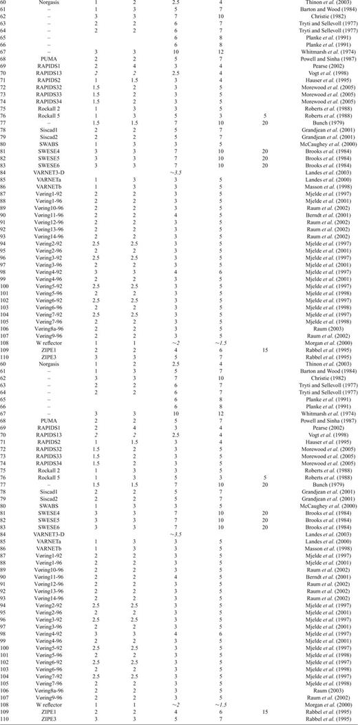
Catalogue of wide-angle reflection/refraction profiles used in the data base.
REFERENCES
