


Summary
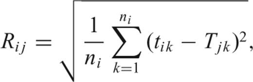
We develop a systematic approach to the phase identification of late-arriving groups in 2-D seismic data. Waveforms in the same traveltime branch are grouped, and synthetic traveltimes for all phases are calculated using an initial approximation to the 2-D structure. For each group, we identify the two synthetic phases providing the smallest RMS residuals. If their ratio is less than some predetermined threshold, then the group's phase is ambiguous and both assignments must be tested by traveltime inversion. If there are n unidentified groups, we construct 2n phase tables and perform a traveltime inversion on every plausible phase assignment. The phase table that provides the highest value of the posterior probability density is taken as correct, and a 2-D velocity model is constructed from the data. This approach is shown to be effective and efficient on both simulated and real data. In addition, the residuals associated with late-arriving groups provide a means of identifying deficiencies in the initial model.
1 INTRODUCTION
Refraction and wide-angle reflection experiments using artificial sources are widely used to reveal the velocity structure of the crust and uppermost mantle in marine experiments. Over the last two decades, many authors have developed methods of inverting wave traveltimes to infer structure (e.g. Zelt & Smith 1992; Hammer . 1994; Toomey, Solomon & Purdy 1994; Zelt & Forsyth 1994; McCaughey & Singh 1997; Mochizuki . 1998; Zelt & Barton 1998). These methods can objectively determine the uncertainty and resolution of derived model parameters by analysing their covariance matrices (or the so-called ‘checkerboard’ tests). Although the technique of traveltime inversion has greatly improved the quality of seismic velocity models, there remain two major barriers for further improvement.
The first lies in constructing the initial 2-D or 3-D models. Because traveltime optimization and fitting are highly non-linear problems, most approaches are highly dependent on the initial model assumptions. Inversion results may be trapped in local minima or become unstable if the proper initial model is not used. The second problem is encountered during the phase identification of a given traveltime. The later arrivals are very useful in improving the resolution of the model, but a wave should only be included in the inversion if it can be confidently identified (Zelt 1999). Because it can be quite difficult to distinguish later arrivals, most authors have used only first arrivals (e.g. Mochizuki . 1998; Zelt & Barton 1998) or later waves that can be unambiguously recognized by visual inspection (e.g. Zelt & Smith 1992).
To solve the former problem, we have developed a new inversion method based on the progressive model development method (PMDM), which uses the traveltimes of refracted waves to derive the 2-D velocity structure of the medium (Sato & Kennett 2000). PMDM consists of three steps. (1) 1-D continuous velocity models are constructed using a genetic algorithm for each side of each receiver (for marine experiments) or shot (for land experiments). This simple inversion is then used to construct a pseudo-2-D continuous velocity model using the turning point approximation. This model is used to infer the number and general location of layer boundaries. (2) Using the inferred number and general location of layer boundaries derived in step 1, we search for 1-D layered models on each side of each receiver. These are then used to construct a pseudo-2-D layered model. The purpose of this step is to provide a rough idea of the 2-D layered structure. (3) Starting from a smoothed version of the 2-D layered model derived in step 2, we construct an accurate 2-D model using a Bayesian, non-linear, iterative traveltime inversion. Since steps 1 and 2 both use inversion (except to determine of the number and general location of layer boundaries), step 3 allows us to construct the proper initial model for a fully 2-D inversion. The major drawback of current PMDM implementations is their exclusive use of first arrivals to derive the velocity models.
This paper presents a systematic approach to identifying later arrivals and using them in the analysis of seismic refractions and wide-angle reflections. The resulting models thus have higher resolution. Since this approach does not require visual inspection, the estimated structures are more objective and the validity of initial assumptions can be quantitatively assessed.
2 SYSTEMATIC PHASE IDENTIFICATION AND INVERSION
Our initial model of the 2-D layered structure is generated from first arrivals, using the current implementation of PMDM as described in the introduction. This model is then refined using later arrivals via the following process.
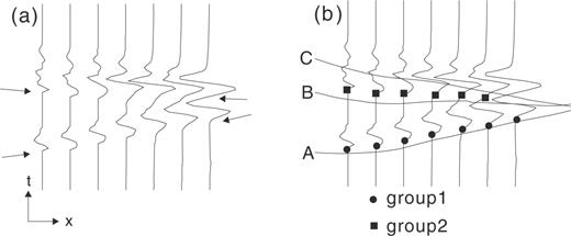
Schematic diagrams demonstrating grouped arrival data and the synthetic traveltimes of three phases. (a) A seismogram showing two traveltime branches (indicated by arrows). (b) Picked data groups based on the traveltime branches (circles and squares), and the traveltimes of three synthetic phases (A, B, C) calculated from an initial model.
Fig. 1(b) shows an example of two data groups (1, 2) and three synthetic traveltime branches (A, B, C). Let us first consider group 1. Phase A clearly produces the smallest RMS residuals (rms1), while phase B provides a second minimum (rms2). Because phase A is very close to group 1 the ratio rms2/rms1 is large, and we can unambiguously associate phase A with group 1. In contrast, phases B and C have similar time residuals with respect to group 2. This may indicate that the initial model does not accurately represent the true velocity structure.
To determine which phase is more representative of group 2, we carry out two traveltime inversions using fixed phases for the picked data, similar to the method used by Zelt & Smith (1992). The phase of each arrival must be assigned (whether correctly or not) before the inversion is performed. Thus, one inversion will use a table in which phase B corresponds to group 2, while the other uses a table in which phase C corresponds to group 2. In both phase tables, however, phase A corresponds to group 1. The inversion that provides the larger value of the posterior probability density function is selected as more representative of the group phase.
When there are several unidentified groups, many inversion calculations must be performed. If the number of unidentified groups is n, the number of possible phase tables is 2n. The phase table that produces the largest value of the posterior probability density function is used to derive the velocity model.
Note that visual inspection plays a role only in data picking and grouping. Although the above procedure requires large amounts of computation, the identified phases are reliable and objective because the inversion calculations are conducted for all reasonable alternatives.
3 NUMERICAL SIMULATION
To judge the quality of the procedure described above, we simulate a generalized marine experiment with many artificial sources and a network of ocean bottom seismometers. The test model is shown in Fig. 2. Layers 1 and 2 are the water and the sediment layers. Layers 6 and 7 have a convex-upward structure. We parametrize the structure following the RAYINVR method (Zelt & Smith 1992), which produces a layered representation of the 2-D isotropic velocity structure with variable block sizes. Each layer boundary is specified by an arbitrary number and arrangement of nodes connected by linear interpolation. The velocity field is specified independently in each layer, by an arbitrary number and arrangement of nodes specified at the upper and lower boundaries. Within a layer the velocities at arbitrary points are calculated by linear interpolation proposed in Zelt & Smith (1992), but the velocities may be discontinuous across a boundary. The inversion parameters are the depths of the layer boundaries and the velocities of the layers, holding the horizontal positions of boundary and velocity nodes fixed. In this analysis, we simulate an experiment with seven receivers and sources spaced every 2 km. Synthetic seismograms, constructed using the Maslov asymptotic method (Chapman & Drummond 1982), are shown in Fig. 3.
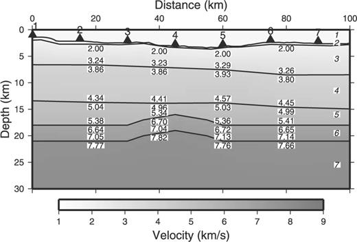
Test model structure. The lines indicate layer boundaries. P-wave velocities (in km s−1) are shown in plain text, and layer numbers are shown in italics. Layer 1 is seawater (1.5 km s−1), and layer 2 is sediment (1.7 km s−1 at the top, 1.8 km s−1 at the bottom). Numbered triangles indicate the receivers.
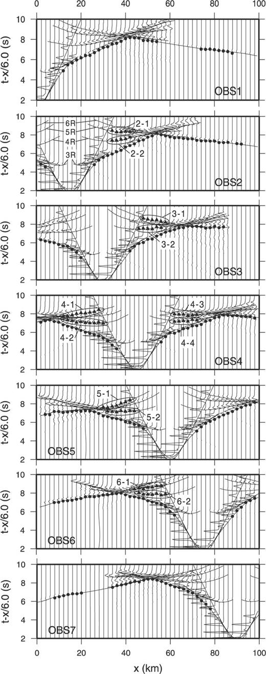
Synthetic seismograms and picked data. Circles indicate first arrivals, and triangles indicate later arrivals. Groups of later arrivals are indicated by ellipses and labelled with their group number. The solid lines are traveltime curves. 3R, 4R, 5R and 6R denote rays reflecting from the lower boundaries of layers 3, 4, 5 and 6, respectively. Some artificial noise due to endpoint error (Chapman & Drummond 1982) is added to the synthetic seismograms.
First arrivals and later arrivals were picked from each receiver. Gaussian noise with a standard deviation of 0.05 s was added to the picked data; the noisy data are represented by circles and triangles in Fig. 3. Later arrivals were grouped based on traveltime branches, as previously described. This resulted in 2 groups for receivers 2, 3, 5 and 6 and 4 groups for receiver 4. Thus, there are a total of 12 groups arriving after the first.
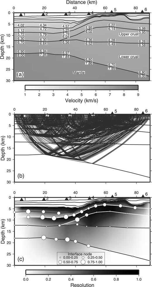
Simultaneous with the grouping of later arrivals, the current implementation of PMDM (Sato & Kennett 2000) was used to construct an initial 2-D model (Fig. 4). The PMDM model does not reproduce the convex-upward structure of layers 6 and 7, and the resolution of the boundary between layers 4 and 5 is poor. Taking the PMDM model as a starting point, we calculate synthetic traveltimes for all refraction and reflection phases. Here again we use the RAYINVR method (Zelt & Smith 1992).
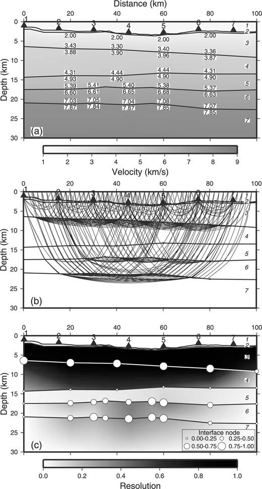
Results of PMDM using only first arrivals. (a) Estimated structure. (b) Ray paths using PMDM. (c) Resolutions of the interface nodes and velocity nodes, using the diagonal elements of the resolution matrix. A value of one means that the parameter is completely resolved, while a value of zero means that the parameter is completely undetermined. Larger circles represent better resolution for interface nodes, and darker shading represents better resolution for the velocities.
Table 1 shows the phases with the two smallest RMS residuals associated with each group, and the ratio between their residuals rms1 and rms2. Only in two groups (3–1 and 5–1) did the true phase correspond to rms2 rather than rms1. We can see from this example that setting the limit of rms2/rms1 to 3 singles out four groups (2–1, 3–1, 4–1 and 5–1) for a systematic search. The other groups will be assigned the phase corresponding to rms1.
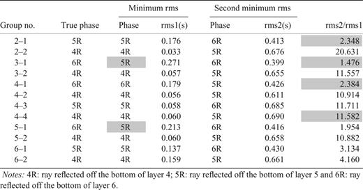
Minimum and second minimum rms phases for late-arriving groups.


In these equations s(m) represents the total variance, m the parameters of the new estimated model, d the traveltime data, and T(m) the traveltimes calculated for m. Cd is the covariance matrix of the data, m0 is the initial set of model parameters, Cm0 is the covariance matrix of m0, and c is a constant. For simplicity, we assume that Cd is a diagonal matrix composed of the variances di. The initial information (m0 and Cm0) is obtained from the PMDM model. Our iterative algorithm for the inversion is similar to that developed by Jackson & Matsu'ura (1985), which allows estimation of both the covariance and the resolution of the model. Partial derivatives of the model parameters for each iteration are calculated using the RAYINVR method (Zelt & Smith 1992).
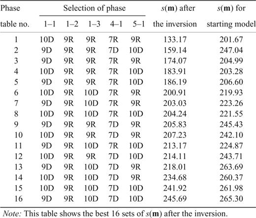
Table 2 reports the value of s(m) for all 16 inversions, in increasing order. (Smaller total variances s(m) correspond to larger values of the posterior probability density.) The phase table with the minimum s(m) is the same as the true phase table (No. 1, group2–1:phase5R, 3–1:6R, 4–1:6R, 5–1:6R) In contrast, note that the phase table with the minimum s(m) relative to the starting model (No.11, 2–1:5R, 3–1:5R, 4–1:6R, 5–1:5R) does not also provide a post-inversion minimum of s(m).
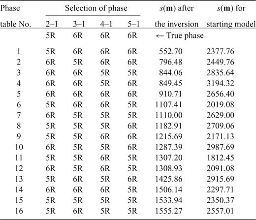
Result of the systematic inversion .
This result means that the systematic search described here is an effective means of determining the best phase model. The relative consistency of phase identification can be estimated from the inversion sets. In the top four options of Table 2, for example, groups 3–1 and 5–1 are identified with phase 6R (reflection from the bottom of layer 6) three times and 5R (reflection from the bottom of layer 5) only once. Group 2–1 is identified with phase 5R in the best phase table, but with phase 6R in the following three entries. This means that the consistency of phase identification is relatively high for groups 3–1 and 5–1.
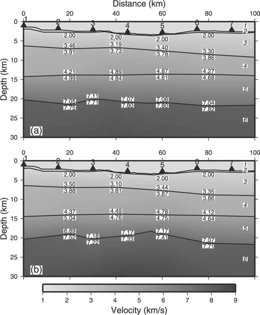
Fig. 5 shows the revised model structure obtained by using the best phase table. This model successfully reproduces the convex-upward structure of layers 6 and 7. Its resolution is also much higher than that of the starting model (Fig. 4), especially at the boundary between layers 4 and 5. In contrast, Fig. 6 shows the model estimated using the phase table with the smallest s(m) relative to the initial PMDM model (No. 11). This model does not reproduce the convex structure of layers 6 and 7. The phase table closest to the starting model does not always provide good results.
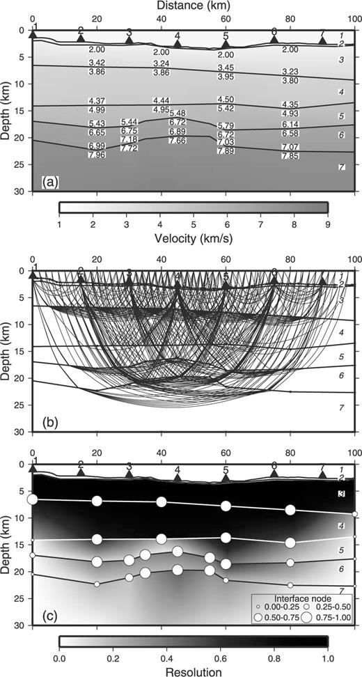
Results of the systematic inversion. This model is derived from the phase table that minimizes s(m) after the systematic inversion. (a) Estimated structure. (b) Ray paths. (c) Resolution values of the interface and velocity nodes.
A model derived from the phase table that provides the minimum s(m) with respect to the starting model. (a) Estimated structure. (b) Ray paths. (c) Resolution values of the interface and velocity nodes.
It is clear from these results that later arrivals are very effective in improving structural models. However, incorrect phase identifications may lead to an incorrect structural interpretation. Fortunately, the quality of the phase table and its associated velocity model can be objectively assessed by a systematic evaluation of all the reasonable alternatives.
4 APPLICATION OF THE SYSTEMATIC INVERSION TO REAL DATA
The previous section has shown that the systematic inversion of all possible phase identifications can effectively determine the correct phase of late-arriving groups, and thus improve the quality of artificial velocity models. In this section, the procedure is applied to real data and its results are compared to those derived from manual phase evaluation and modelling by trial-1135-error.
We use data obtained from a seismic refraction/reflection survey conducted in the Japan Sea (Sato . 2006). The objective of this survey was to investigate the transition zone between oceanic and continental velocity structures, and thereby shed light on the formation of the Japan Sea. The survey was conducted using six ocean bottom seismometers (OBS) and a towed airgun array. Sato . (2006) modelled the seismic structure using a combination of the PMDM method, the RAYINVR method (Zelt & Smith 1992), and trial-1135-error forward modelling. Obtaining the final model was a very lengthy process, due to the time spent identifying the phases of later arrivals.
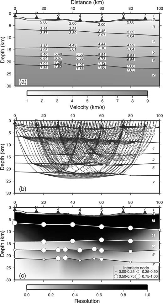
Fig. 7 shows the data observed by each OBS and the picked group arrivals (points). The priorities of group 1 in OBS 1 and group 2 in OBS 4 cannot be identified with certainty, so these two groups are treated as later arrivals and their proper phases are determined during the systematic inversion. A 2-D structure is estimated first, using PMDM and unambiguous first arrivals exclusively (Fig. 8). The well-defined shallow velocity structure (at depths less than 3–4 km) was estimated by Sato . (2006) based on the reflection profile and refraction survey. The resolution of the deep velocity structure (lower crust and the Moho boundary) is poor due to the low number of first-arrival rays passing through the lower crust and the upper mantle.
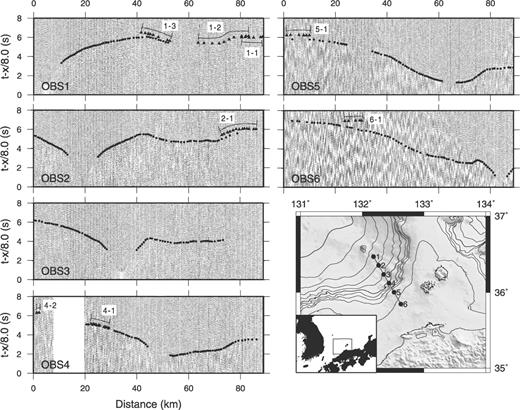
Real seismograms and picked data from a seismic survey of the Japan Sea. Circles indicate the first arrivals, and triangles indicate later arrivals (as interpreted by Sato . 2006). Groups of later arrivals are indicated by lines and labelled with their group number.
The PMDM model for the Japan Sea data, using only first arrivals. (a) Estimated structure. (b) Ray paths using PMDM. (c) Resolution values of the interface and velocity nodes.
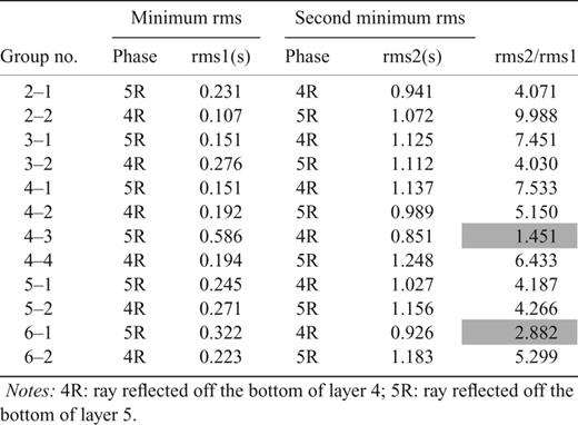
Table 3 shows the two best phases for each group, and the ratios rms2/rms1. Five groups have an rms2/rms1 ratio less than 3, so 25= 32 phase tables are constructed for the systematic inversion.
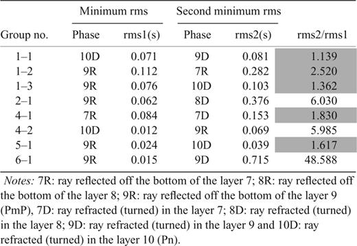
Minimum and second minimum rms phases for late-arriving groups of the real data.
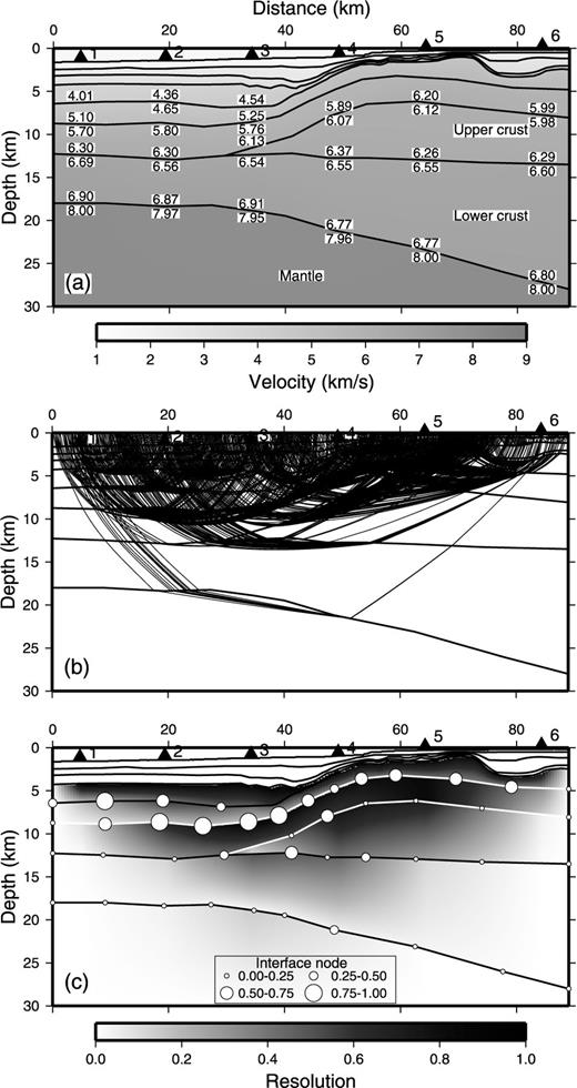
Table 4 and Fig. 9 show the results of the systematic inversion. Including later arrivals increases the number of rays passing through the lower crust and the upper mantle substantially, greatly improving the resolution of the deep velocity model. The eight best phase tables show that the identification is relatively consistent for groups 1–2 and 4–1. The phases of the later arrivals are the same as those eventually chosen by trial-1135-error (Sato . 2006), so the velocity structure derived from the systematic inversion process is essentially identical to the model constructed by Sato et al.
Result of the systematic inversion for the real data.
Results of systematic inversion for the Japan Sea data. This model is derived from the phase table that minimizes s(m). (a) Estimated structure. (b) Ray paths. (c) Resolution values of the interface and velocity nodes.
The inversion of a single phase table requires 5–10 min of computation time on a PC-Linux workstation with a 2 GHz Celeron CPU, so the total time required in this case is 3–5 hr. The systematic method performs as well as trial-1135-error phase identification with forward modelling, but also provides a quantitative and objective analysis of the results and errors. Furthermore, it requires much less time than manual methods.
5 DISCUSSION
The systematic inversion of all possible phases for later arrivals represents an efficient and rapid approach to deriving the best velocity model from 2-D refraction/reflection data. In the previous section, however, note that we used a good initial model produced by PMDM. To investigate the limitations of this approach, we now consider an example using a poor initial model.
Using the simulation of Section 3 (Fig. 3), we construct an artificial six-layer structure created by combining layers 5 and 6 (Fig. 10a). The systematic inversion procedure is then carried out using this as the initial model. Table 5 shows the two best phases and the ratios rms2/rms1 for all late-arriving groups. Two groups have an rms2/rms1 ratio less than the predetermined limit of 3, so only four phase tables are required for the systematic inversion.
(a) Estimated model using PMDM with an incorrect six-layer structure. The first arrival data are the same as those shown in Fig. 3. (b) Results of systematic inversion using Fig. 10(a) as the initial model.
Minimum and second minimum rms phases for late-arriving groups using a poor initial model.
Fig. 10(b) shows the model that provides the minimum s(m) after inversion. It does not reproduce the true convex-upward structure, but this test still reveals that the later groups may provide a useful check on the quality of the initial model. Table 6 compares the RMS residuals for later arrivals found in the good and poor initial models, calculated using the best model in both cases. In the case of the poor initial model, four groups (4–1, 4–3, 5–1 and 6–1) had RMS residuals exceeding twice the standard deviation of 0.05 s. In the good initial model, no group had an RMS residual greater than 2 standard deviations. This result suggests that when a large number of groups have RMS residuals greater than 2 standard deviations, we should consider reconstructing the initial model.
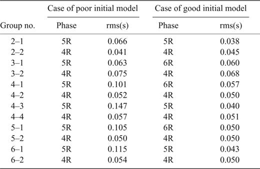
RMS for later arrival groups calculated from the best model.
Another limitation on this method is that high-quality data sets are needed to produce the initial velocity structure and to pick and group late-arriving phases. The data sets used in the previous examples are quite dense, with many rays sampling the volume under consideration. The procedure outlined above may not be appropriate for data sets with low ray density or poor coverage. The procedure discussed in this paper should probably also be restricted to data sets with high resolution at the reflection or turning points of late-arriving rays.
Significant computation time may be required when there are many unidentified groups. Inverting 16 phase tables (four unidentified groups) requires only 2–3 hr. For n= 10, however, 1024 inversions may take 4–7 d on a standard workstation. This problem can be resolved by parallelization, because each inversion computation is completely independent of the others.
Even parallelization may be insufficient, however, if the number of unidentified groups is larger than 10. One may be able to solve this problem by subdividing unidentified groups into ‘families’ based on their reflection or turning points, as determined from ray path analysis. Then the phase identification can be carried out within each family while holding the phases of all other families constant. For example, if 20 unidentified groups are subdivided into four families of five groups each, the number of required inversion sets is only 25× 4 =128 instead of 220. In this manner the computation time can be greatly reduced with little loss of resolution or efficacy.
Global search algorithms can also be applied in cases where there are very large numbers of unidentified groups. For example, the phase tables used in the present approach could easily be represented as binary strings, and the optimal phase table found using a genetic algorithm (e.g. Sambridge & Drijkoningen 1992). If the minimum rms phase is represented by 0 and the second minimum rms phase is represented by 1, the best phase table in the numerical simulation found in Table 1 can be represented as 0101. Computation time can be greatly reduced by using a genetic algorithm to optimize the solution.
In the above examples, we set a heuristic threshold of 3 on the rms2/rms1 ratio. In practice, this value needs to be determined by users based on the character, quality, and density of their data set. Further investigation is required before the appropriate value of this limit can be determined from first principles. In the meantime, we propose carrying out the systematic inversion once with a small value of the threshold (2 or 3), then again with a somewhat larger value. If the two limits result in the same phase identification, the value may be appropriate. If not, further inversions should be carried out with successfully larger limits until the phase identification stabilizes.
We have not discussed how best to determine the number and arrangement of nodes in the model, choosing to focus on explaining our systematic approach to phase identification. The appropriate number of nodes will depend on the specific application. One approach is to set up an underdetermined model, with many nodes and some smoothness constraints on the model parameters. In non-linear problems, the weights of the constraints may be determined using the scheme developed by Constable . (1987). Their scheme is that the smoothest model which fits the experimental data to within an expected tolerance is sought, rather than fitting the experimental data as well as possible.
6 CONCLUSIONS
The systematic inversion of all possible phase identifications for later arrivals is a rapid and objective approach to deriving the best velocity model. The essence of this approach lies in determining the two phases which provide the smallest RMS residuals for each late-arriving group; this allows us to identify ambiguous groups and perform inversions on a well defined and limited set of possible phase tables. This approach may not perform well if the initial velocity model is poor; however, this can be checked using standard statistical procedures by evaluating the residuals of the groups. This inversion method may also require high-density data sets, with good ray coverage of the volume under investigation. When there are many unidentified groups, computation times may also become unreasonably large. Alternative computing solutions can alleviate this problem, including: (1) parallelization, (2) subdivision of the unidentified groups into families with similar reflection or turning points and (3) using a genetic algorithm to search for the optimal phase table.
ACKNOWLEDGMENTS
The author thanks Takeshi Sato for providing data from the Japan Sea survey. This paper has been improved by comments from Y. Ben-Zion, J. Fletcher and an anonymous reviewer. The figures were generated using the GMT software developed by the University of Hawaii (Wessel & Smith 1998). This work was supported by JSPS (Grants-in-Aid for Scientific Research, 12640401). The programs associated with this work will be made available. See
REFERENCES
Notes: 4R: ray reflected off the bottom of layer 4; 5R: ray reflected off the bottom of layer 5 and 6R: ray reflected off the bottom of layer 6.
Notes: 7R: ray reflected off the bottom of the layer 7; 8R: ray reflected off the bottom of the layer 8; 9R: ray reflected off the bottom of the layer 9 (PmP), 7D: ray refracted (turned) in the layer 7; 8D: ray refracted (turned) in the layer 8; 9D: ray refracted (turned) in the layer 9 and 10D: ray refracted (turned) in the layer 10 (Pn).
Note: This table shows the best 16 sets of s(m) after the inversion.
Notes: 4R: ray reflected off the bottom of layer 4; 5R: ray reflected off the bottom of layer 5.
