


Summary
We implement the wave equation on a spherical membrane, with a finite-difference algorithm that accounts for finite-frequency effects in the smooth-Earth approximation, and use the resulting ‘membrane waves’ as an analogue for surface wave propagation in the Earth. In this formulation, we derive fully numerical 2-D sensitivity kernels for phase anomaly measurements, and employ them in a preliminary tomographic application. To speed up the computation of kernels, so that it is practical to formulate the inverse problem also with respect to a laterally heterogeneous starting model, we calculate them via the adjoint method, based on backpropagation, and parallelize our software on a Linux cluster. Our method is a step forward from ray theory, as it surpasses the inherent infinite-frequency approximation. It differs from analytical Born theory in that it does not involve a far-field approximation, and accounts, in principle, for non-linear effects like multiple scattering and wave front healing. It is much cheaper than the more accurate, fully 3-D numerical solution of the Earth's equations of motion, which has not yet been applied to large-scale tomography. Our tomographic results and trade-off analysis are compatible with those found in the ray- and analytical-Born-theory approaches.
1 INTRODUCTION
One of the important challenges in seismology is to enhance the tomographic resolution of the Earth's interior. A way to achieve this goal is by elaborating more accurate theoretical descriptions of seismic wave propagation and using them to formulate the tomographic inverse problem. The Born approximation (single-scattering theory) represents a possibly significant improvement with respect to simple ray theory; for some time now it has been known to be valid at least for weak scattering in the Earth (Hudson & Heritage 1981; Wu & Aki 1985). On the basis of the Born approximation, the ‘banana–doughnut’ paradox, or the prediction that the sensitivity of seismic traveltime observations be maximum away from the ray-theoretical path, was pointed out most clearly by Marquering (1999) (but see also Kennett 1972; Woodhouse & Girnius 1982; Snieder 1987; Snieder & Nolet 1987; Li & Tanimoto 1993; Li & Romanowicz 1995); numerous studies have been made to understand the nature of this phenomenon (Dahlen 2000; Hung 2000; Zhao 2000; Spetzler & Snieder 2001; Spetzler 2002; Baig 2003; Tanimoto 2003; Baig & Dahlen 2004; de Hoop 2005; Tromp 2005).
The Born approximation, while representing an improvement with respect to simple ray theory, cannot reproduce non-linear effects that take place in reality (Wielandt 1987; Nolet & Dahlen 2000; Hung 2001; Baig 2003). In addition, implementations of Born theory found in the literature are typically based on far-field expressions of the wavefield, giving rise to singularities in the computed Fréchet derivatives (sensitivity kernels) (Favier 2004). In practice, the forward problem is formulated under the assumption that scattering occurs only at distances from source and receiver much larger than the wavelength, but its solution is then used to compute the values of sensitivity kernels in the vicinity of source and receiver as well, where the kernels are actually singular. This singularity appears to be integrable (Friederich 1999, Appendix E), but it remains unclear to what extent these asymptotic kernels are valid near the source and receiver. Capdeville (2005) proposed an efficient way to overcome this problem in the computation of sensitivity kernels, combining adjoint methods (Tromp 2005, and references therein) and normal mode summation, though his approach has not yet been applied in practice to the inversion of real seismic data.
Direct numerical integration of the equations of motion is another way to avoid the far-field approximation, and simulate, at least to some extent, the non-linear phenomena mentioned above. Computational power has grown tremendously in recent years thanks to a combined improvement in processor performance and in size of multi-processors clusters (Bunge & Tromp 2003; Boschi 2007); over the last decade, the average growth-1098-year in the computational performance of supercomputers has slightly exceeded Moore's law, which predicts a factor of 2 in 18 months (Strohmaier 2005). Seismologists with access to large parallel computers are now able to calculate seismic waves propagating through a 3-D, complex medium closely resembling the Earth. Nevertheless, such simulations can take quite a long time even for a single earthquake and on large cluster systems; for example, Tsuboi et al.'s (2002) simulation of the Denali earthquake in a very realistic earth model took about 15 hr on one of the fastest supercomputers in the world. It is therefore, too time-consuming to perform the large number of full numerical integrations required to set up an inverse problem numerically unless one simplifies the problem (e.g. Tape 2007).
Here we explain how the 3-D problem of fundamental-mode surface wave propagation is represented by a 2-D, zero-thickness membrane analogue. We then use the membrane wave analogue to compute sensitivity functions relating surface wave phase measurements to lateral anomalies in the phase velocity of surface waves. This is a notoriously time-consuming endeavour, but we reduce its cost through the application of an adjoint-method approach (e.g. Tarantola 1984) similar to that of Tromp (2005). We apply the sensitivity functions in an inversion of real data to derive phase-velocity maps of the Earth, which we compare in the last part of this work with those obtained from ray-theory and analytical Born-theory tomography (e.g. Spetzler 2002; Boschi 2006).
2 THE FORWARD PROBLEM: MEMBRANE WAVES
Membrane waves as an analogue for surface waves were introduced by Tanimoto (1990), to investigate locally the strong effects of lateral heterogeneity on short-period surface waves (10 and 20 s). We follow the same approach to derive a numerical model for the propagation of intermediate-period surface waves at the global scale, which requires special spherical grids and numerical techniques (e.g. Sword 1986). In the interest of simplicity, we give only a detailed theoretical treatment of the Love-wave case below. Working with a Rayleigh wave Ansatz leads to an algebraically more complicated, but qualitatively analogous derivation (Tanimoto 1990; Tromp & Dahlen 1993).
2.1 Theory

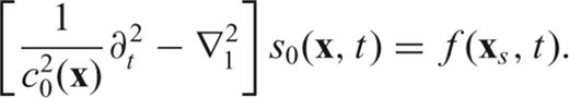
 denoting the unit vector, ∇1 the surface gradient (e.g. Dahlen & Tromp 1998) and s(ϑ, ϕ) a scalar ‘potential’ at colatitude ϑ and longitude ϕ. It follows that for an isotropic stress–strain relation and in the smooth-Earth approximation, s satisfies

2.2 Meshing the Earth's surface
It is impossible to evenly distribute more than 20 points on the surface of the sphere, a distribution of points describing a platonic dodecahedron. Modelling on the sphere at regional scale lengths requires thousands of points, and thus the grids will have at least some undesired irregularities. Spherical geodesic grids of triangular faces, first introduced in the context of meteorological flow modelling (Sadourny 1968; Williamson 1968), are one approach to the non-trivial problem of uniformly discretizing the Earth's surface (Cui & Freeden 1997; Saff & Kuijlaars 1997).
In practice, the sphere is first discretized by a platonic solid, that is, a regular polyhedron consisting of identical cell faces. We find the initial triangular mesh combining the vertices of a dodecahedron and an icosahedron (Tape 2003), also known as a truncated icosahedron or a buckyball. We then refine the grid iteratively, using the midpoints of the three sides of each spherical triangle to divide it into four new smaller triangles, forming the next finer grid. This method will be referred as dyadic refinement (Baumgardner & Frederickson 1985). The corresponding hexagonal/pentagonal (in the following loosely referred to as hexagonal) grid is constructed from the triangular grid. The corner of each hexagonal or pentagonal face is found by calculating the central point of each spherical triangle from the corresponding triangular grid. Vertices of the triangular grids then coincide with the cell centres of the hexagonal grids.
As we shall show in the next section, s is evaluated at the vertices of the triangular grid, while the computation of its Laplacian involves the areas of the hexagonal grid cells, so that the properties of both grids are relevant to our implementation. Comparisons in Table 1 show that our hexagonal grid has a more uniform distribution than others based on the icosahedron as the initial triangular grid (e.g. Heikes & Randall 1995a; Wang & Dahlen 1995). A further improvement of the distribution could still lead to an even more accurate numerical solution; in the next section we show that our hexagonal grid is sufficiently good to provide a valuable basis for the numerical computations.
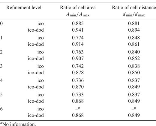
Properties of spherical grids. Comparison between spherical grids based on icosahedral (ico) and icosahedral-dodecahedral (ico-dod) initial platonic solids. The membrane wave calculations use the hexagonal grid based on the second combination of two platonic solids (ico-dod). Values for the icosahedral case are taken from the twisted grid used by Heikes & Randall (1995a).
2.3 Finite-difference scheme
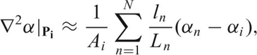
Eq. (7) shows that the calculation of the Laplacian for a given cell requires only information on the neighbouring cells. This is why this scheme is said to be a ‘local’ method, in contrast to other ‘global’ numerical implementations like the spectral methods mentioned above. The advantage of local methods is that they can be parallelized in a very efficient way.

We explain this effect introducing ‘grid distortion’ as the distance between the midpoint of the segment connecting two neighbouring cell centres, and the midpoint of the corresponding cell edge, divided by the cell edge length (Heikes & Randall 1995b, section 2). At each cell, we average grid distortion over all its neighbours, and plot the result in Fig. 1(a). When the plotted value is zero, the cell is symmetric and the grid is not distorted at the corresponding location. We find the Laplacian to be nearly second-order accurate at most gridpoints (see also Heikes & Randall 1995b). A few cells exist with a particularly high distortion (∼2 per cent or less). Table 1 confirms, nevertheless, that our grid is more uniform (hence, less distorted) than alternatives found in current literature.
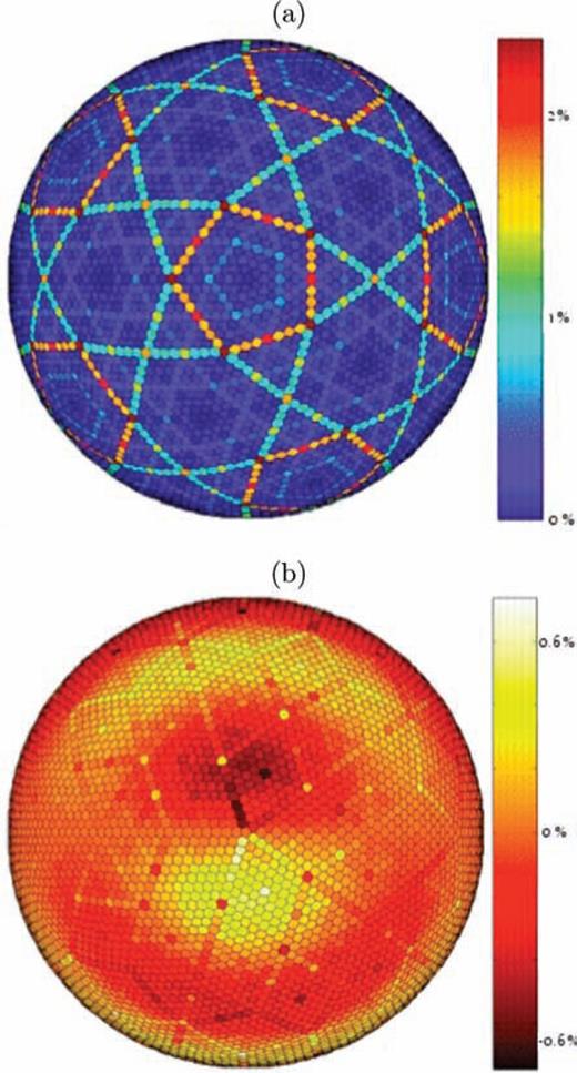
Properties of the hexagonal grid. (a) Distortion measured by the midpoint ratio of distance between cell centres and cell edges to corresponding cell edge length (Heikes & Randall 1995b). (b) Accuracy of Laplacian for a spherical harmonic function (l= 6, m= 1). Differences between numerical and analytical values are normalized to the maximum value of the analytical Laplacian. View from North Pole down projected onto the equatorial plane.
Fig. 2 shows a snapshot of the scalar potential solution to the wave eq. (3) derived numerically over the whole sphere. Fig. 3 shows the resulting scalar potential solutions and phaseshifts between the analytical and numerical solutions for Love waves at 150 s period. Phaseshifts are shown for filtered and unfiltered solutions; the simple source mechanism described by eqs (5) and (6) excites a wider range of frequencies, which have to be filtered out in order to isolate the frequency of interest. We examine this in more detail in Section 3.3.2
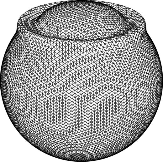
Snapshot of wave propagation on the spherical membrane for a source at the North Pole. Wavefield s is plotted on a spherical-triangular grid with 7682 vertices.
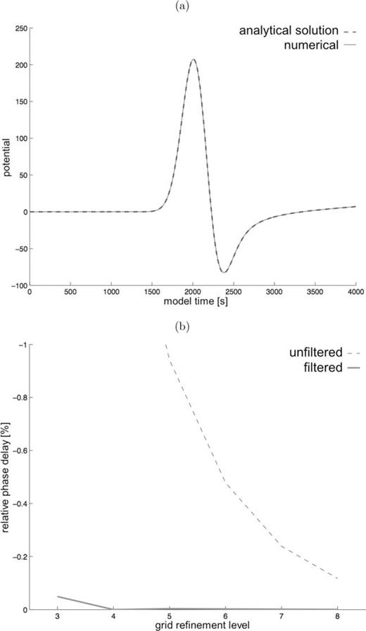
Accuracy of numerical membrane waves. (a) Analytically (dashed) and numerically (solid) calculated membrane wave s, generated from a source at (0°N, 0°E) and recorded at (0°N, 90°E). (b) Phase-shift between the analytical and numerical, filtered (solid) and unfiltered (dashed) solutions shown in (a), for different levels of grid refinements. Filtering is discussed in Section 3.3.2
We find that differences between the analytical and numerical solutions are small enough that the numerical algorithm can be considered valid, and can be applied to evaluate the effects of small lateral heterogeneities, or formulate a tomographic inverse problem. We conduct numerical integrations on the grid defined by six successive dyadic refinements, yielding 122 882 hexagonal or pentagonal cells. On the basis of Fig. 3, we consider this mesh a good compromise between the cost of further refinements, and inaccuracies introduced by making the grid coarser. The grid spacing, or average distance between the centres of neighbouring cells, is ∼70 km, corresponding to about 10 gridpoints per dominant wavelength for the reference case of 150 s period waves.
 is the average phase velocity of the model. Simulations with a time step smaller than (13) will require a longer computation time without increasing the precision. The time step also limits the sampling rate of modelled waves; in Section 4, we will apply a quadratic interpolation between sampled times to cross-correlate accurately our computed traces (e.g. Smith & Serra 1987; Press 1992).
2.4 Computational considerations
The main advantage of collapsing a 3-D problem to two dimensions is an order-of-magnitude gain in the speed of simulations. Our software is parallelized to optimize its performance on a Linux cluster. We use the implementation MPICH of the standard message passing interface on a 16-processor cluster. Software performance on parallel computers depends on the amount of communication between different processes needed during a simulation. If no communication were needed, the calculation time would decrease linearly as a function of the number of available processors. The more communication required, the slower the performance will get, and, above a certain number of processors, no further gain in speed will be possible.
Table 2(a) shows how the performance of our implementation scales with respect to the number of processors. It can be seen that if the latter is doubled, runtime decreases by a factor of ∼2. Above eight processors, the gain in speed falls off. Note that in principle we should expect the simulation time to increase by a factor 8 for a next finer grid, as there will be four times more grid cells due to the dyadic refinement, and the number of time steps will double due to a halving of the space step. Table 2(b) shows the runtimes for single simulations conducted with different grid spacings employing 16 processors in parallel. A single simulation, running in parallel on clusters larger than ours, will nevertheless be punished by the need of data communication between the processes. Since one simulation can be completed within a minute on a single processor (for grid spacings around 70 km), a large cluster system has the obvious advantage that each processor can run a separate simulation.
Performance efficiency. Runtimes with (a) different numbers of processors and an average grid spacing of 70 km, (b) 16 processorsa, different grid spacings.
A single simulation of surface wave propagation via the full numerical integration of the equation of motion in 3-D (e.g. spectral-element methods) would take minutes even on large cluster systems, and can be carried out in seconds by our approximate, 2-D membrane wave algorithm on a small cluster. While analytical methods like that of Spetzler (2002) are only proved to perform well in a spherical-background-Earth scenario, we show below that ours, through an application of the adjoint method (Tarantola 1984), can provide a full kernel library in a heterogeneous reference model as well, in a reasonable amount of time.
3 MEMBRANE–WAVE SENSITIVITY FUNCTIONS
3.1 A ‘direct’ approach

Note that numerical integration of eq. (3) on the membrane involves a simplified representation of the source in terms of initial displacement and source–time function (Section 2.1). We must therefore, neglect the effects on wave propagation of specific seismic source mechanisms (Zhou 2004; Yoshizawa & Kennett 2005). This will be the subject of further investigations.
In principle, calculating K(ϑi, ϕi) for each cell i requires as many simulations as there are cells. This exercise then has to be repeated, in the case of a homogeneous reference Earth [constant c(ϑ, ϕ)], for a dense set of epicentral distances spanning the range of true epicentral distances at which observations are available. In the case of a laterally heterogeneous reference Earth, it has to be repeated for each combination of source and station locations for which observations are available. The latter endeavour is too costly and we have discarded it; however, in the case of a constant reference phase velocity, it is feasible to calculate kernels via eq. (17).
3.1.1 Geometrical setup
We reduce the number of simulations needed to find K(ϑ, ϕ) in the ‘direct’ approach as follows (Tong 1998): after placing the source at, say, the North Pole, we perform one simulation for each scatterer location along one chosen meridian (Fig. 4). For each simulation, we save modelled traces at an array of receivers located along the parallels, spaced 1° in longitude and latitude from each other. If the background earth model is homogeneous, what matters is not the absolute locations of scatterer and receiver, but their relative positions. From the set-up described above, we therefore, find the same traces that we would find considering one receiver at a time, and performing one simulation per possible scatterer location.
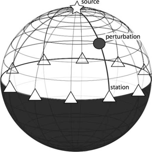
Set-up for the ‘direct’ approach to computing sensitivity kernels (Section 3.1.1), with one source (star) located at the North Pole, the scatterer position (circle) varying along a single meridian, and a set of receiver stations (triangles) located along parallels.
In practice, this results in reducing the number of required simulations from 64 442 to 181 (for the reference case of 1°× 1° sampling of K(ϑ, ϕ), and using 360 receivers simultaneously). Running our parallel algorithm on 16 processors, with a gridspacing of about 70 km (level six hexagonal grid), we entirely determine K(ϑ, ϕ), for a given epicentral distance, in about 6 min. Without the simplification introduced here, the same computation would take approximately 3 d.
3.1.2 Non-linearity
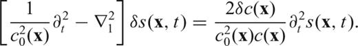
In principle, sensitivity functions derived as in Section 3.1 should not depend on the value of the imposed phase-velocity perturbation γ. However, as γ grows, the problem eventually becomes non-linear, and the linearized eq. (14) ceases to be valid, together with the concept itself of sensitivity kernels. Testing the stability of our algorithm, we have found that, above a certain threshold (γ∼ 2 per cent), the mentioned non-linearity comes into play and numerical kernels we find are slightly but visibly affected by changes in the value of γ.
Hung (2001) found a similar effect from a set of 3-D spectral element simulations. In their fig. 17 they plot traveltime anomaly found by cross-correlation (equivalent to our δΦ) as a function of imposed heterogeneity (γ in Section 3.1 here, ɛ in Hung 's (2001) notation). While Born theory requires that a linear relationship exists between δΦ and γ, the corresponding curve obtained from numerical results is a straight line only for small values of γ. Hung (2001, section 5.6) find an asymmetry in the dependence of δΦ on γ for positive versus negative values of γ. They explain this result as a combination of wave front healing and the ‘overhealing’ effect of the cross-correlation technique. In our case there is not such a strong asymmetry between the effect of negative and positive anomalies.
3.2 The adjoint approach
Our ‘membrane’ algorithm is efficient enough that, on a homogeneous reference Earth, K(ϑ, ϕ) can be computed by a large set of direct simulations. The number of simulations required to determine K(ϑ, ϕ), however, is much larger when the reference Earth is laterally heterogeneous, and the ‘direct’ approach outlined above ceases to be practical. Tromp (2005) give an overview of the application of backpropagation to the calculation of sensitivity functions, resulting in the ‘adjoint methods’ introduced by Tarantola (1984) or Talagrand & Courtier (1987). In this approach, regardless of the complexity of the reference model, K(ϑ, ϕ) for a given source–receiver pair can be fully determined with two simulations only: one for the forward-propagating wavefield, from the source to the receiver; another for the backpropagating wavefield, from the receiver to the source. At each point (ϑ, ϕ), K(ϑ, ϕ) is found algebraically as a function of the forward- and backpropagating wavefields.
Next we provide a formulation of the adjoint method for the case of surface wave phase-anomaly observations, to be inverted tomographically in our spherical membrane approach. Part of our treatment is very similar to that of Yoshizawa & Kennett (2005, section 2), except that we prefer to work in the time domain; the rest follows Tromp (2005, sections 2 and 4.1).
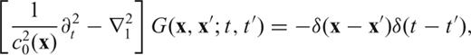
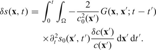
3.2.1 Writing displacement anomalies in terms of the Green's function

 to both sides of (18),

3.2.2 Writing traveltime (or phase) anomalies in terms of the Green's function
 (which coincide with relative perturbations in phase), this implies
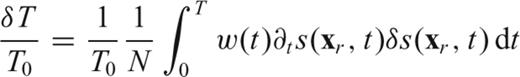
3.2.3 Finding membrane sensitivity kernels in the adjoint approach
 coincides with the wavefield originated on the membrane by a source
 and
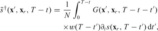
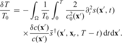
and  ‘adjoint field’ and ‘adjoint source’, respectively. Note that the adjoint source is by definition located at the receiver xr, and that it contains the time-reversed velocity seismogram from the forward synthetic wavefield.
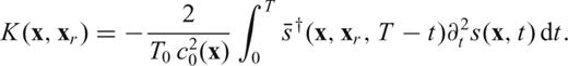
The practical relevance of eqs (31)–(34) becomes apparent when one realizes that (31) can be implemented numerically, feeding  as defined by (34) to a numerical algorithm like our finite-difference membrane scheme, reversed in time. One forward-propagating simulation must be conducted previously, so that s(xr, t) be known (its first and second derivatives with respect to time can be determined numerically): the adjoint source is then entirely defined, and one more run of the finite-difference algorithm is sufficient to determine K(x, xr), for all values of x. Whatever the source-station geometry, and the complexity of the starting model c0(x), K(x, xr) is known after two simulations only.
3.3 Some practical considerations
3.3.1 Discretization of the adjoint source
 (subscript m for membrane) of
  as defined by eq. (34),
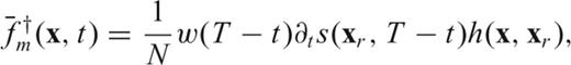
 the adjoint field generated by
  on the discretized membrane. Then, by definition of Green's function,
 , it makes sense to use (40) and replace
  with
with  in (33), to find an expression for the discrete version Km of sensitivity kernels
3.3.2 Waveform filtering
While we are interested in the propagation of one mode (one frequency of the dispersive surface wave packet) at a time, our membrane analogue is excited over a range of frequencies, depending on the initial conditions (5) and (6). To isolate the mode of interest, we bandpass-filter the solution using as centre frequency the frequency of the mode of interest, and a half-bandwidth of 2.5 mHz. Spetzler (2002) average their sensitivity kernels over the same bandwidth, to account for the fact that single-frequency phase-velocity measurements are not possible, owing to the finite sampling of seismograms and to the finite parametrization of the dispersion curve in the measurement process. The selected value for bandwidth also coincides with the spacing between splines parametrizing the measured dispersion curves in Ekström (1997, fig. 1), which could be taken as a rough estimate of the accuracy of said dispersion curves (Boschi 2006).
As noted in Section 2.1, each membrane simulation provides the surface wave potential s associated with one specific surface wave mode. Strictly speaking, only the component of s at the frequency of the mode of interest is then physically meaningful. The relatively large bandwidth of our bandpass filter leads, however, to an effect similar to that found analytically by Spetzler (2002), reducing the amplitude of kernels' sidelobes. Filtering can be equivalently applied to the scalar potential s found by numerical integration on the membrane, or to the initial conditions (5) and (6). We have experimented with both approaches, obtaining practically coincident results. The latter option is naturally more efficient.
4 RESULTS
The discussion that follows is limited to phase-velocity kernels of intermediate-to-long period Love waves; we expect that a similar procedure is valid, and the same qualitative results hold for the case of Rayleigh waves.
4.1 Sensitivity kernels for a homogeneous (spherical-Earth) starting model
4.1.1 Comparing analytically and numerically determined sensitivity kernels
In Fig. 5, we compare a sensitivity kernel calculated numerically in the membrane approach, with one calculated analytically from Boschi's (2006) implementation of Spetzler 's (2002),eq. (16), based on Snieder & Nolet's (1987) single-scattering approach. Source (0°N, 0°E) and receiver (0°N, 90°E) locations, and surface wave period (150 s) are the same in both cases. The background value for phase velocity coincides with the Love-wave, PREM-based (Dziewonski & Anderson 1981) value. Numerical kernel values are calculated on the cell midpoints (as described in Section 2.3) of our grid and then interpolated for plotting with 1° spacing in both latitude and longitude. Analytical values are likewise averaged over each cell and interpolated for plotting.

Sensitivity kernel for Love waves at 150 s, spherical earth model (homogeneous phase velocity), source at (0°N, 0°E) and receiver at (0°N, 90°E), (a) calculated numerically in the ‘direct’ approach; (b) calculated implementing the analytical formula of Spetzler (2002).
As pointed out by Favier (2004) and Boschi (2006), Spetzler 's (2002) and other Born-theory formulations (e.g. Zhou 2004; Yoshizawa & Kennett 2005) involve a far-field approximation of the unperturbed solution; sensitivity kernels found in this approach are necessarily singular at source and receiver. This explains the unphysical behaviour of analytical kernels evident from Fig. 5(b) at longitudes around 0° and 90°. Furthermore, analytical kernels in Fig. 5 are zero at longitudes larger than the epicentral distance, and at any location at a negative azimuth from the source; this is an effect of simplifications in Spetzler 's (2002) procedure—a fictitious feature that we do not find in expressions for analytical kernels later derived by Zhou (2004) and Yoshizawa & Kennett (2005).
4.1.2 Comparing sensitivity kernels found via the ‘direct’ versus adjoint approach
In Fig. 6, a comparison between cross-sections of numerical kernels for Love waves at 150 s period is shown. Numerical kernel values are either calculated with the ‘direct’ approach or the adjoint method, both described in Section 3. We employ in both cases the same numerical mesh and homogeneous background model. For the ‘direct’ approach, we apply a relative perturbation γ of −0.2 per cent. Source and station are at a fixed epicentral distance and placed as in Fig. 5. Cross-sections of both kernels are taken at distinct longitudes. The ‘direct’ calculation takes about 6 min on 16 processors to produce a complete numerical-direct kernel over the whole sphere (using the reduction from Section 3.1.1). With the adjoint method, the complete numerical-adjoint kernel is obtained in about 2 min on a single processor. As can be seen, the two kernels are practically identical. This is an important demonstration of the internal consistency of our approaches.
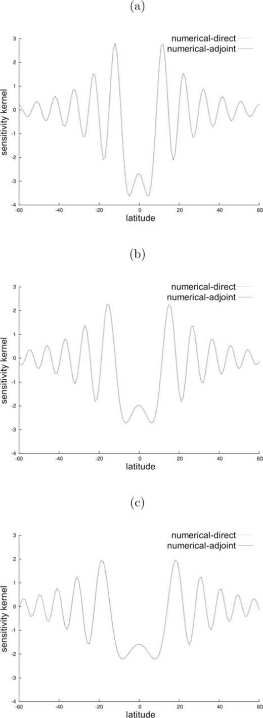
Cross-sections of sensitivity kernels for Love waves at 150 s calculated via the ‘direct’ approach (dashed lines) and adjoint method (solid lines), with source at (0°N, 0°E) and receiver at (0°N, 90°E). Sensitivity values are plotted as a function of latitude only, along three chosen meridians, namely (a) 10°, (b) 20° and (c) 45°.
In Fig. 7, we explore how membrane sensitivity kernels vary as a function of source-station distance; the area of all Fresnel zones expands as already described by, for example, Spetzler (2002, fig. 2b). For stations located closer to the epicentre, overall higher sensitivity is found. Fig. 8 shows the dependence of sensitivity kernels on wave period at a fixed epicentral distance. The central lobes of the kernels increase with increasing period. This is qualitatively confirmed by analytical results (e.g. Spetzler 2002, fig. 2a).
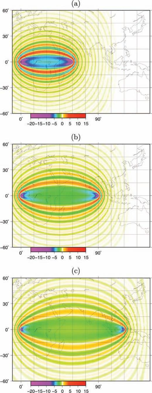
Numerical-adjoint kernels derived for 150 s Love waves in a homogeneous starting model. The source is located at (0°N, 0°E), the receiver at 0°N and (a) 60°E, (b) 90°E and (c) 120°E.
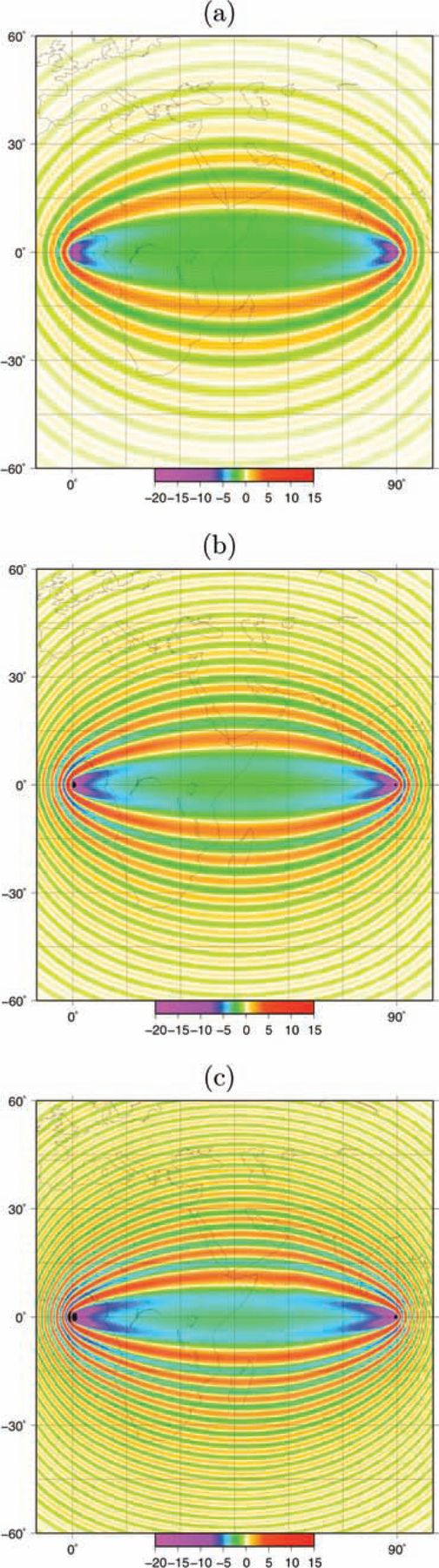
Numerical-adjoint kernels for Love waves at (a) 150 s, (b) 100 s and (c) 75 s periods, in a homogeneous starting model. The source is located at (0°N, 0°E), the receiver at (0°N, 90°E).
Due to the memory-intensive storage of the numerical grid, our current computer hardware prevents us from running simulations with periods <75 s. The numerical scheme we apply requires about 10 nodes per wavelength for an accurate representation of the wave phenomena on the membrane (see Section 2.3); thus, for shorter periods we would need a grid spacing with less than 17 km distance which leads to more than two million grid cells. With 2 GB RAM memory per cluster node we are bound by this limitation. A work-around could consist of accessing the mesh points through I/O with a corresponding file storage. This would considerably slow down the computation process.
4.2 Sensitivity kernels for a laterally heterogeneous starting model
Our method naturally allows us to calculate phase-velocity sensitivity kernels associated with a laterally heterogeneous starting model (background Earth). Computing a single numerical kernel in the adjoint approach takes exactly the same time (2 min on one of our processors) regardless whether the background Earth is homogeneous or heterogeneous. In the limit of our smooth-Earth assumption, we explore the impact of background heterogeneities on the properties of surface wave kernels.
Fig. 9 shows a starting model for 150 s Love wave phase velocity. We derived it based on local normal-mode theory (Boschi & Ekström 2002), from an earth model consisting of the 3-D crustal model Crust-2.0 (Bassin 2000), overlying a 1-D, radially isotropic profile of the mantle as in Boschi (2004). The map in Fig. 9 represents a rough guess of crustal effects on long-period Love wave propagation, and is independent of surface wave observations like those we will invert in the following. In order to expect significant differences, it has been filtered to harmonic degrees ≤40 (thus allowing spatial wavelengths close to the ones of Love waves at 150 s). Our implementation is only physically meaningful in the smooth-Earth approximation (Section 2.1); the algorithm remains stable in the presence of strong gradients, but the formulation of the membrane approach depends upon lateral smoothness.
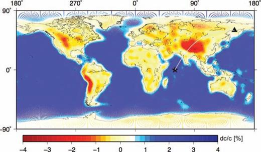
150 s Love-wave phase-velocity map based on Crust-2.0 (Bassin 2000) and an isotropic upper-mantle model. The phase-velocity heterogeneities are represented by a spherical harmonic expansion with degrees l≤ 40, resulting in a low-pass filtered phase-velocity map (the membrane analogue has physical meaning in a smooth Earth regime). Phase-velocity values are projected onto our hexagonal grid, and plotted as coloured dots at the centre of each of its cells (122 882 total cells). Source and receiver are denoted by the star and triangle connected by the source–receiver great circle, which crosses the Tibet anomaly. Phase-velocity anomalies are given in percent with respect to PREM.
We show in Fig. 10(a) a 150 s Love wave kernel based on the model of Fig. 9, and a source-station geometry that should maximize the effect of the starting model's strongest phase-velocity heterogeneity, located in the Himalaya region with approximately −3 per cent relative phase-velocity perturbation. The homogeneous-Earth kernel associated with the same source and receiver is shown in Fig. 10(b), and the difference between the two in Fig. 10(c). The two kernels coincide in the first Fresnel-zone (main lobe), while significant differences are apparent in the sidelobes. Strongest differences are found to the southeast of the great circle path, corresponding to higher gradients in phase velocity (transition from a continental to an oceanic region).
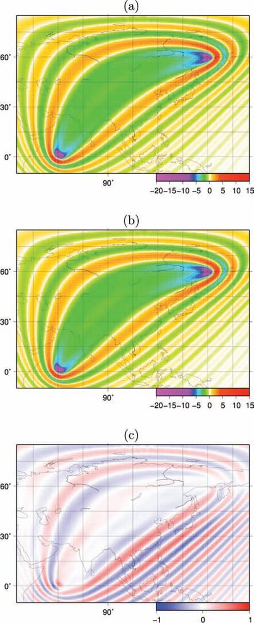
Sensitivity kernels derived with the adjoint method for 150 s Love waves in (a) homogeneous and (b) heterogeneous (Fig. 9) starting phase-velocity models. (c) Difference between (a) and (b).
4.3 A test of the first-order scattering approximation
Born theory is a single-scattering theory, that is, it neglects the interaction of scattered wavefields with other heterogeneities. In practice, the linearized, Born-theoretical eq. (14) implies that the effect of multiple heterogeneities be equal to the sum of the independently calculated effects of each heterogeneity. In forward calculations made on a smooth earth model, our numerical algorithm naturally accounts for multiple scattering. Hence, while we do not attempt to formulate an inverse problem accounting for multiple scattering, we can perform a set of forward calculations to evaluate its relevance, and the associated inaccuracy of the linearized Born approximation.

In the approach (i), multiple scattering is implicitly accounted for; in the approach (ii) it is neglected. The linearized Born approximation would suggest that both values of δΦjk are identical; differences between the resulting phase anomalies are the effect of multiple scattering. We perform a number of simulations with: source and receiver located at (0°, 0°) and (0°, 90°), respectively; one scatterer located at 45° longitude, and at latitudes varying between −60° and 60°; a second scatterer at the same latitude, and at a longitudinal distance of +3°, +6° or +9° to the first. For each considered couple of scatterers, we find phase anomaly both by ‘direct’ numerical calculation [approach (i)] and by eq. (42)[approach (ii)]; we plot in Fig. 11 the difference between the resulting values of δΦ as a function of scatterer-latitude.
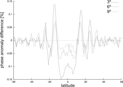
Effects of multiple scattering. We use the membrane-wave method to calculate the phase anomaly δΦnumi resulting from two scatterers, located at the same latitude and longitudinal distances 3°, 6° and 9°, and source and receiver at (0°N, 0°E) and (0°N, 90°E), respectively. After each simulation, we subtract δΦnumi from the phase anomaly δΦBorni by simple Born theory (no multiple scattering, but the sum of the individual effects of each scatterer) and normalize the result to the maximum value of δΦBorni from all our multiple-scattering simulations. The resulting quantity (δΦBorni−δΦnumi)/max{δΦBorni} is plotted in percent vs. scatterer latitude, with a separate curve for each value of longitudinal distance between scatterers (3°: solid line, 6°: long-dashed line, 9°: short-dashed line).
As a general rule, we find that the effects of multiple scattering on seismic phase are small and the linearization in eq. (14) is valid. The largest discrepancy in δΦ amounts to ∼0.15 per cent of the maximum δΦ predicted by eq. (42) and corresponds to the smallest distance (3°) between the two scatterers. These values are so small that the shape of the curves is significantly affected by the irregularity of the grid: gridpoints do not precisely align along parallels, but can be shifted up to ±0.5° in our mesh and the curves in Fig. 11 are jagged as a result. Multiple scattering becomes even less relevant for larger interscatterer distances (6° and 9° in our experiment). The latter result is to be expected, as the energy of the scattered wavefield at a given point decreases with increasing distance from the scatterer, by simple geometrical spreading. We infer that in a smooth-Earth regime the Born linearization is valid in the tomographic determination of phase-velocity anomalies. It would become less reliable at longer times/higher orbits.
4.4 Application to fundamental-mode surface wave tomography

We invert the database of Ekström (1997), updated as described by Boschi & Ekström (2002), implementing (44) and least-squares solving (43) with the algorithm of Boschi (2006), but calculating K(ω, ϑ, ϕ) in different ways and different starting models, as described below. Our phase-velocity maps are linear combinations of equal-area pixel functions as in Boschi (2006). The coverage (see Fig. 12 for 150 s Love-wave observations) and resolving power of the Harvard dispersion database have been evaluated in earlier publications (e.g. Ekström 1997; Carannante & Boschi 2005).
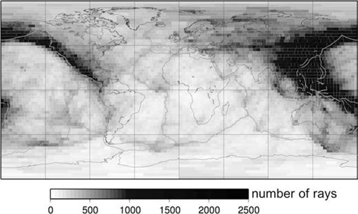
Ray-theoretical hitcount map (number of rays crossing each pixel) from the Harvard database, 150 s Love wave observations only. The equal-area pixel parametrization (3°× 3° at the equator) is the same used in our inversions.
4.4.1 Tomography with a homogeneous starting model
We follow the procedure described in Sections 3.2 and 3.3 to calculate sensitivity kernels K(ω, ϑ, ϕ) defined by eq. (14)[strictly speaking, what we find and use is their ‘discretized version’Km(ω, ϑ, ϕ) defined by (41)]. So long as the starting model is homogeneous, the function K(ω, ϑ, ϕ) changes if the source–receiver distance changes, but is not affected by changes in the locations of source and receiver: following Boschi (2006), we find K(ω, ϑ, ϕ) at a discrete set of epicentral distances ranging from 20° to 179°, with 1° increments. We later spline-interpolate (Press 1992) calculated K(ω, ϑ, ϕ)’s to find K(ω, ϑ, ϕ) for any epicentral distance (Boschi 2006). In analogy with Spetzler (2002) or Boschi (2006), we neglect source-mechanism variations for different events in the database, and use the source term (5), (6).
After implementing eq. (44) for the entire database at a chosen surface wave mode, we least-squares invert (43) a number of times, varying the value of the roughness-damping parameter (Boschi 2006; Boschi 2006); no other regularization constraint is applied. The resulting L-curve, or plot of misfit versus normalized roughness of the solution, as defined by Boschi (2006), is shown in Fig. 13(a). While we experimented with a variety of surface wave modes and tomographic parametrization, we shall limit our discussion to 150 s Love wave data inverted on a grid of equal area pixels with surface extent 3°× 3° at the equator.
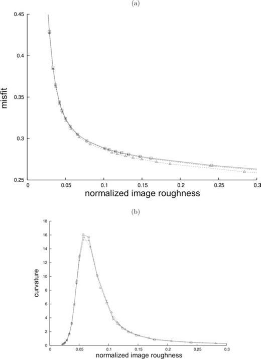
Trade-off analysis for the phase-velocity inversions of Section 4.4.1 (homogeneous starting model). (a) L-curves for solutions derived from ray theory (dotted line, triangles), analytical Born theory (dashed line, pluses), and numerical-adjoint kernels (solid line, squares). (b) Curvature of the curves shown in (a). Image roughness is defined and normalized as in Boschi (2006).
We repeat this exercise, employing alternatively ray-theoretical sensitivity kernels, and analytical Born-theoretical ones based on Spetzler (2002). We find that the L-curves resulting from the three approaches are qualitatively similar, as also noted by Boschi (2006). We identify from Fig. 13(b) solutions corresponding to equal curvature of the associated L-curves, and roughness comparable to that of, for example, Ekström (1997). Associated phase-velocity maps are shown in Fig. 14. The results of the three approaches are remarkably similar; the only discrepancies worth mentioning are perhaps two fast anomalies of small lateral extent, in the southeastern part of the Chinese Gansu province and in the Andes, present in the analytical-Born-theory solution, but not in the other two.
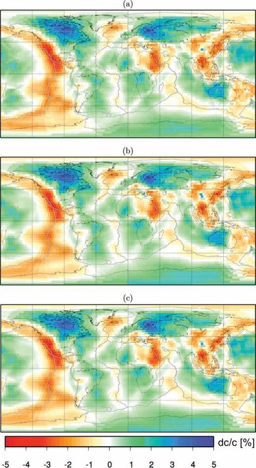
Phase-velocity maps from the inversions of section 4.4.1 (homogeneous starting model). We compare solutions found from (a) ray theory, (b) analytical Born theory, (c) numerical-adjoint kernels. Phase anomalies are in percent with respect to the value predicted by PREM.
The most time-consuming part of our experiment was the calculation of sensitivity kernels at the mentioned set of 160 epicentral distances, for one surface wave mode (150 s Love waves). Applying the adjoint method on one processor, this would last about 5 hr. Computing Aij for 16 624 observations of δΦ/Φ takes another 5 hr. Finally, least-squares solving the resulting linear inverse problem by means of LSQR, with A relatively dense, for a large set of roughness-damping parameter values takes a further 3 hr.
4.4.2 Tomography with laterally heterogeneous starting models
As discussed in Section 4.2, in a laterally heterogeneous Earth the form of a sensitivity function K(ω, ϑ, ϕ) depends not only on epicentral distance, but also on the specific locations of source and receiver. For this reason, K(ω, ϑ, ϕ) has to be calculated for each source–receiver pair, that is, for each observation in the database. At the speed of currently available hardware, this would be practically impossible if the ‘direct’ approach algorithm of Section 3.1 were used. It becomes feasible when the procedure described in Section 3.2 is applied, thanks to the gain in speed achieved with the adjoint approach.
We limit ourselves, again, to Love-wave phase-anomaly observations at 150 s, and use as a starting phase-velocity model the one of Fig. 9, based on the crustal model Crust-2.0 and an isotropic upper-mantle model (Section 4.2). We next
- (i)
multiply the matrix A found in the homogeneous-model case by the vector of starting-model coefficients, and subtract the resulting phase-anomaly vector from the data; let us denote d′ the resulting, corrected phase-anomaly vector;
- (ii)
following the method described in Section 4.2, compute a sensitivity kernel for each of the 16 624 summary observations (150 s Love waves only) available in the Harvard database; let us denote
 the kernel associated with the i-th observation;
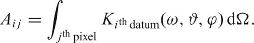
 - (iii) after a kernel is calculated, augment the matrix A′ accordingly; the ij entry of A′ is naturally definedwith the same pixel grid used in previous inversions (approximately equal-area pixels, 3°× 3° at the equator);45

- (iv)
iterate the two previous steps until A′ accounts for all available data;
- (v) dubbed x′ the coefficients of perturbations to the starting model of Fig. 9, least-squares solve the linear inverse problemrepeatedly, for a wide range of values of the roughness damping parameter (again, no other regularization constraint is applied);46

- (vi)
conduct a trade-off analysis to identify a preferred solution model, whose regularization is compatible with that applied in earlier experiments, so that the results can be compared (Boschi 2006).
The L-curve and its curvature resulting from the trade-off analysis (vi) are shown in Fig. 15(a) and (b), respectively, as functions of normalized image roughness. The L-curve of Fig. 13 derived by numerical-adjoint kernels is also shown in Fig. 15 for comparison. Starting the inversion from a heterogeneous model, derived from Crust-2.0 and a spherically symmetric upper-mantle model (Fig. 9), leads to solutions with a worse datafit than the homogeneous-starting-model ones of equal roughness, suggesting that the chosen heterogeneous model does not describe sufficiently well the propagation of Love waves at 150 s period. As in this approach the starting model has non-zero roughness, the corresponding L-curve does not tend to zero for decreasing model complexity, but converges to the roughness value of the initial starting model.
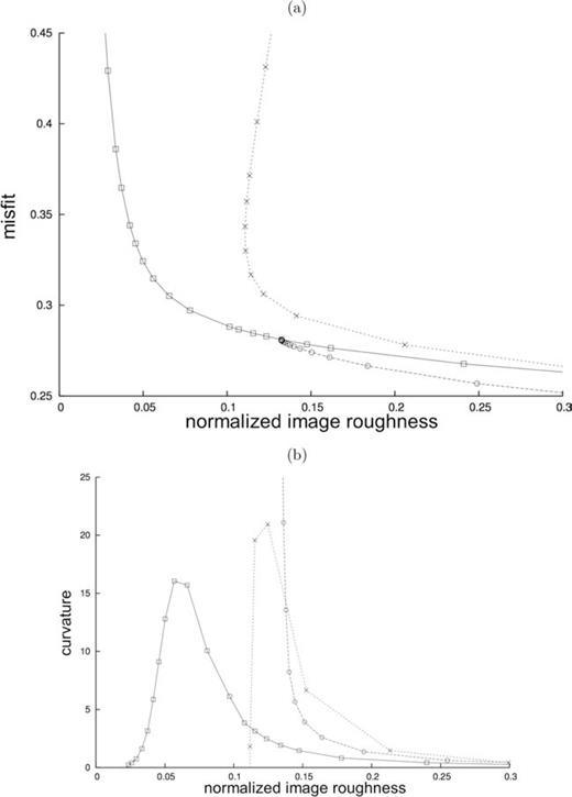
Trade-off analysis for the phase-velocity inversions of Sections 4.4.1 and 4.4.2 (heterogeneous starting model). (a) L-curves for solutions derived using numerical-adjoint kernels based on three different starting models: a homogeneous starting model (solid line, squares) (curve repeated from Fig. 13); the heterogeneous starting model shown in Fig. 9, which itself was derived from Crust-2.0 and an isotropic upper-mantle model (dotted line, crosses); the heterogeneous starting model shown in Fig. 14c, which itself was derived using numerical-adjoint kernels (dashed line, circles). (b) Curvature of the curves shown in (a).
We repeated this exercise, using as a starting model the one shown in Fig. 14(c), derived from the inversions using numerical-adjoint kernels. This represents a first iteration step in a non-linear inversion scheme where the zeroth iteration starts with a homogeneous phase-velocity model. Steps (ii), (iii) and (iv) are the most time-consuming and took about 22 hr using 16 processors in our cluster. Step (v) takes about 3 hr on a single processor, as in the homogeneous-model case: this is not surprising since A and A′ are equally dense. The solutions obtained have a slightly better fit to the data than from the zeroth iteration. We iterated the process one more time, to find only insignificant changes in model and misfit.
The points of equal curvature in Fig. 15(b) (dotted line/crosses, dashed line/circles) identify our preferred solutions, which we show in Fig. 16. We first combine x′ with the starting model (of Fig. 9 and Fig. 14c, respectively), so that heterogeneities are again defined with respect to the value of 150 s Love-wave phase velocity predicted by PREM. Only few, small differences between the maps of Fig. 16 and those of Fig. 14 are apparent. Namely, in the top panel of Fig. 16 a fast, southeastern Atlantic anomaly can now be distinguished from the fast anomalies corresponding to cratons in western and southern Africa; the same happens in South America, where the fast anomaly in the southern Atlantic Ocean is more clearly separated from the Brazilian one. Using Crust-2.0 as a starting crustal model in a 3-D, ray-theoretical inversion, and then computing phase-velocity maps associated with the resulting 3-D shear velocity model, a similar effect is observed (unpublished result by L. Boschi, 2006, based on the method of Boschi & Ekström 2002 and Boschi 2004).
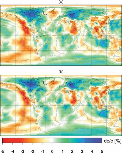
Phase-velocity maps derived from inversions based on two different heterogeneous starting models. In each case the inversion employed sensitivity kernels calculated via the adjoint method for each respective heterogeneous model. In (a), the starting model is the phase-velocity map of Fig. 9, which was based upon Crust-2.0 and an isotropic upper-mantle model (see Section 4.2). In (b), the starting model is the phase-velocity map of Fig. 14(c), which was derived using numerical-adjoint kernels (see Section 4.4.1).
We show in Fig. 17 the power spectrum up to degree 40 of the phase-velocity maps in Figs 14 and 16. All spectra strongly resemble each other, particularly at lower harmonic degrees (longer spatial wavelengths). Note that the phase-velocity maps obtained from laterally heterogeneous starting models (based on Crust-2.0 and an isotropic upper-mantle model; and based on an initial inversion from PREM) show slightly higher spectral values at degrees >5.
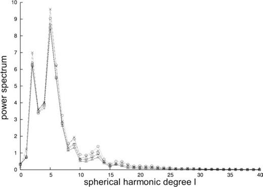
Harmonic spectra of models from Figs 14 and 16. The power spectra are taken from the phase-velocity maps shown in Fig. 14, which were derived from a homogeneous starting model by ray theory (solid line, triangle), analytical Born theory (dashed line, pluses) and numerical-adjoint kernels (short-dashed line, squares), as well as the phase-velocity maps shown in Fig. 16, which were derived from the heterogeneous model shown in Fig. 9 (dash–dotted line, crosses) and Fig. 14(c) (dotted line, circles) employing numerical-adjoint kernels.
5 CONCLUSIONS
We model surface wave propagation in a smoothly heterogeneous Earth, implementing the wave equation numerically on a spherical membrane (zero thickness). The numerical method utilizes a finite-difference scheme specifically designed for the spherical grids. In comparison with existing techniques, our approach has both advantages and disadvantages. It is less accurate than the fully 3-D, numerical solution of the Earth's equations of motion (e.g. Komatitsch 2002; Capdeville 2003) in that it requires the smooth-Earth/no-mode-coupling approximation to be made, but an order of magnitude faster. Unlike the analytical approaches like those of, for example, Spetzler (2002); Zhou (2004) and Yoshizawa & Kennett (2005), it does not involve any far-field approximation (Favier 2004), and accounts for some of the non-linearities of wave propagation in a realistic medium (Tanimoto 1990). Zhou 's (2004) method, on the other hand, considers also mode coupling. Both Zhou 's (2004) and Yoshizawa & Kennett's (2005) methods account for the effects of seismic source radiation, which our membrane analogue does not.
The high speed of our finite-difference membrane wave algorithm, combined with the application of the adjoint method (e.g. Tarantola 1984; Tromp 2005), allowed us to use our membrane analogue to derive sensitivity kernels relating surface wave phase-anomaly data to phase-velocity heterogeneities. We computed sensitivity kernels using two different approaches—one employing adjoint methods, the other using a large set of direct calculations (no backpropagation)—and found coincident results (Fig. 6). We then calculated sensitivity kernels both in a homogeneous and a laterally heterogeneous starting model of phase velocity, and employed them in a set of global inversions of the Harvard dispersion database (e.g. Ekström 1997). Kernels calculated in this way are free from the far-field approximation often used in analytical Born theory (e.g. Dahlen 2000; Spetzler 2002; Boschi 2006). Fundamental-mode tomographic images and trade-off analyses (Figs 13 and 14) derived from different approaches (ray theory, analytical Born theory, numerical Born kernels) are approximately coincident (see also Fig. 17).
As explained in Section 2, our membrane wave formulation of surface wave propagation relies on the assumption that lateral heterogeneities in upper-mantle structure are relatively smooth. In the near future, we shall extend our numerical-adjoint method approach to 3-D earth models, where the only limit to possible Earth's complexity resides in the accuracy of its numerical discretization, and it will be easier to account for the specific geometry of seismic sources—neglected here—and definitions of phase anomaly more realistic than simple cross-correlation—employed here as a first approximation. Recently published applications of analytical finite-frequency methods to surface wave tomography (e.g. Zhou 2004, 2005) suggest that the 3-D problem overcomes inherent ray theoretical assumptions made when inverting for 2-D phase-velocity maps as in this study; it will take account of depth-dependent radiation patterns for single scatterers. We therefore, expect the 3-D experiment to bring an improvement in data fit and model quality, more significant than what was found here.
ACKNOWLEDGMENTS
We thank Domenico Giardini for his support and encouragement, Yann Capdeville and Jeroen Tromp for their many insightful comments. We are grateful to Göran Ekström for making his dispersion database available to us. We would also like to thank T. Tanimoto, B. Romanowicz, G. Laske and an anonymous reviewer for critical and constructive comments. Funding for this project is provided by the European Commission's Human Resources and Mobility Program Marie Curie Research Training Network SPICE Contract No. MRTN-CT-2003-504267. Carl Tape's master thesis (Tape 2003) is available at
REFERENCES
aNo information.
aProcessor type: AMD Opteron 64-bit, 2 GHz clock speed.
