Maximum entropy regularization of time-dependent geomagnetic field models Free

Summary

1 INTRODUCTION

The evolution of the geomagnetic field takes place over a wide spectrum of timescales ranging from 10–10³ yr for secular variation to 10⁵–10⁶ yr for polarity reversals (Merill 1996). Numerical simulations of convective dynamos in rapidly rotating spherical geometry are now able to reproduce the primary (large lengthscale) features of the Earth's magnetic field and its long term evolution. Despite the limitations of the numerically accessible parameters, these help to provide mechanisms for the geodynamo process (Kono & Roberts 2002). A problem is however presented by the wide variety of dynamo behaviour found in numerical simulations and observed in planetary magnetic fields (Jones 2003). This diversity makes it difficult to reach a comprehensive understanding of the geodynamo. More detailed observational knowledge of the spatial structure and temporal evolution of the geomagnetic field is needed to help distinguish the true mechanisms underlying the generation and evolution of the Earth's magnetic field.

Databases of observations of the Earth's magnetic field, developed from modern sources, historical sources (Bloxham 1989; Jonkers 2003) or archaeomagnetic sources (Korte 2005), have lead to construction of continuous models of the magnetic field at the core–mantle boundary (CMB) from decadal timescales (Sabaka 2004; Olsen 2006) to historical (Bloxham & Jackson 1992; Jackson 2000) and millennial timescales (Korte & Constable 2005). It is well known that given a finite data set, many possible models can be found that fit the data equally well (Backus & Gilbert 1970). To avoid this issue some recent models minimize not only the fit to the data, but also a measure of field complexity. This procedure (known as regularization or damping) leads to simpler—and perhaps more realistic—models, and avoids overfitting of the data (Parker 1994). A variety of norms have been used to measure complexity in field models, many of which have been quadratic functions. All quadratic norms tend to heavily penalize small length-scale field structure, causing a loss of contrast in the reconstructed picture of the field. Their use involves a priori assumptions concerning the field structure, and introduces artificial correlations (for a simple demonstration see the well known ‘kangaroos’ argument for example in Sivia & Skilling 2006, p. 111–112). Furthermore, the minimization of a quadratic norm of the magnetic field at the CMB is not a procedure derived from any fundamental physical law, so that one cannot argue that any specific quadratic norm is ‘the’ relevant measure of field complexity.

In the 1980s the maximum entropy image reconstruction method was developed (Gull & Skilling 1984; Skilling 1988, 1989; Gull 1989). Entropy, in this information theory context, is a non-quadratic measure of model complexity that arises from a minimum of a priori assumptions, and which reduces artificial correlations. Its mathematical form (see Section 3.3) can be derived by requiring that any sensible measure of model complexity should have properties of subset independence, co-ordinate invariance, system independence and should scale correctly (Skilling 1988). Further background details are presented in the companion paper by Jackson (2007), hereinafter referred as Paper I. First developed for positive images only, the maximum entropy method was later extended to non-positive fields (Gull & Skilling 1990; Hobson & Lasenby 1998). Recently, Jackson (2003) applied it to reconstruct snapshots of the radial magnetic field at the CMB for the epochs 1980 and 2000, using the Magsat and Ørsted satellite data. The maximum entropy method is known permit high contrast images, with well-resolved maxima and minima. As pointed out by Jackson (2003), sharper pictures of the radial magnetic field at the CMB are of interest, since numerical simulations often present rather sharp concentrations of magnetic field lines (e.g. Rau 2000).

In Jackson (2003) as well as in Paper I the entropy norm was computed in the spatial domain. In the present study we show how to implement it while working in the spectral (spherical harmonic) domain. At the same time we extend the method to the time-dependent problem, and test its ability to model the main field and its secular variation from historical data over the period 1840–1990. The structure of the paper is as follows. In Section 2, we present the main characteristics of the data sets used during this study. In Section 3, we detail the notation and the methods used to invert the data, including both quadratic and maximum entropy regularization techniques. Then in Section 4 we compare the results obtained with the two types of regularization. Finally, in Section 5, we discuss perspectives for the method and implications for our understanding of the dynamics of the Earth's outer core.

2 DATA COMPILATION

In this study we use the same data compilation as was employed by Jackson (2000). However, the time span has been shortened to the interval 1840–1990, where the data coverage and quality is best. This avoids the need to parametrize the axial dipole intensity before 1840, when no intensity data were available (Gubbins 2006). Here, we briefly recall the most important characteristics of each data set. For more detailed information and references, see Bloxham (1989), Bloxham & Jackson (1989), Jackson (2000) and Jonkers (2003). A few statistics concerning the data's temporal distribution and accuracy are presented in order to give a feeling of the constraints provided by the data on the magnetic field models. The major categories of data in the compilation are listed below. The number of data in each category is summarized in Table 1, together with the time interval covered.

1

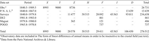
The total number of data and the time span for each data set: X, Y and Z stand for the three Cartesian components of the magnetic field, H, F, I and D stand for the horizontal intensity, total intensity, inclination and declination, respectively.

Open in new tabDownload slide

1. 1

   Survey data: The survey compilation (around 85 per cent of the total amount of data in this study) covers the whole time-span except the last 10 yr. These data have been spatially culled in order to avoid too much correlation from the crustal field arising due to dense local sampling (Bloxham 1989; Jackson 2000). We use a standard estimated error of 200 nT to account for this effect. Note also that some of these data are actually repeat stations that could be used in the future as pseudo-observatory data.

2. 2

   Observatory data: Composed of annual means of the X, Y and Z components of the field at the Earth's surface, these are first differenced in order to become free from the affects of the static crustal magnetization. These data cover the whole time span, though rather few go back to the 19th century. Median values of the estimated errors associated with all three components are, respectively, 5.1, 2.9 and 6.6 nT yr⁻¹. Although these constitute only around 10 per cent of the total amount of data, they provide our best constraint on the time derivative of the field.

3. 3

   Data from the Paris National Library and Archives: These were collected on ships over the first 27 yr of the time span. Composed of declination measurements only (with a median value of the estimated error of 39 min arc), they constitute around 5 per cent of the total number of data.

4. 4

   Satellite data:

   • (i)

     POGO (1965–1970): only quiet time intensity F data were considered (see Langel 1980, for precise details on the selected data), at altitudes from 399 to 1519 km, with typical estimated error of 9 nT.

   • (ii)

     DE2 (1981–1983): only intensity F data were considered (Langel 1988), at altitudes from 248 to 912 km, with typical estimated error of 20 nT.

   • (iii)

     Magsat (1979): quiet time intensity F and vertical Cartesian component Z data were considered, with a Dst correction for the external fields (Langel & Estes 1985), at altitudes from 350 to 575 km, with typical estimated errors of, respectively, 15 and 9 nT for F and Z.

Only satellite data with angular separation greater than 15 degrees have been included to avoid bias from the crustal field (Bloxham & Jackson 1989). Although the satellite data only represent 0.6 per cent of the total amount of data, they provide a very good spatial constraints around 1970 and 1980, in the last 25 yr of the model. This has implications for the modelling since it permits us to build a more complex picture of the field at the end of the time span

The whole data set is then composed of more than 276 000 data, of which nearly 40 per cent are declinations, 20 per cent are horizontal intensities, 10 per cent are total intensities, 15 per cent are inclinations, 15 per cent are Cartesian (northward, eastward or downward) components (see Table 1). We show on Fig. 1 the evolution of the total number of data with time. The sparsity of the data near t_e= 1990, as well as the lack of high quality data near t_s= 1840, have implications for the boundary conditions imposed during the modelling (see the discussion in Section 3.2).

Figure 1

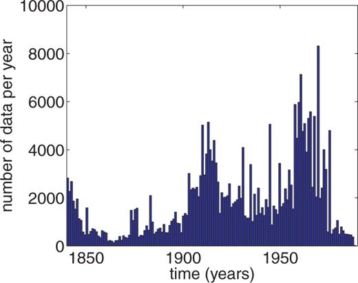
Temporal evolution of the number of data per year, over the period 1840–1900.

Open in new tabDownload slide

3 METHODS AND NOTATIONS

3.1 General framework

Most of the concepts and notation used here are standard (see, for example, Langel 1987). We adopt a spherical coordinate system (r, θ, φ); a= 6371.2 km is the Earth's radius and c= 3485 km is the outer core radius. We assume the mantle is an insulator, so that the magnetic field can be derived from a potential: B=−∇V for r > c. As there are no magnetic monopoles (∇· B=0), we look for the solution of the equation ∇²V= 0. Note that the radial component of the magnetic field B_r entirely describes the potential V for this problem of Laplace's equation with Neumann boundary conditions. The radial magnetic field at the CMB, which we want to reconstruct, is then B_r|_CMB=−∂_rV|_r=c. We use a spherical harmonic expansion of V that can be written for any radius r > c as

1

where the P^m_l are the associated Legendre functions. Regardless of the regularization employed (quadratic or maximum entropy) the same truncation level L= 24 is used throughout this paper. This rather high truncation level enables the undesirable effects produced by over-zealous truncation to be avoided. Note that for l > 13 the core field is dominated by the crustal field at Earth's surface; the field models presented here are controlled only by regularization beyond this point. All models (both quadratic and maximum entropy regularized) converged satisfactorily for l < 24.

We follow Bloxham & Jackson (1992) and use B-splines of order 4 (Lancaster & Salkauskas 1986) as the basis functions to represent the time-dependence of the coefficients g^m_l,

2

with a similar expression for the h^m_l. We use T= 63 B-splines for the temporal representation of the period [t_s, t_e]=[1840, 1990], erected on T+ 4 knots regularly spaced every 2.5 yr. Endpoints were treated by adding three extra knot positions beyond t_s and t_e— trials showed that this produced identical results to using three repeated knots positions at t_s and t_e as is done, for example, by Olsen (2006). 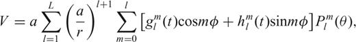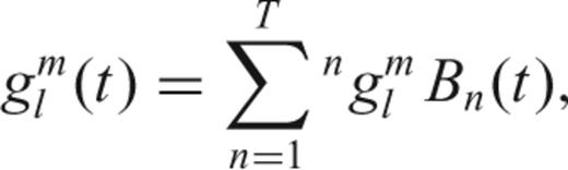In summary, our model consists of a set of P=TL(L+ 2) = 39 312 free parameters to represent the spatial structure and temporal evolution of the CMB field.

The complete set of observations γ, comprising N data, is related to the model m through a forward function f, and we therefore, wish to find solutions to the problem . Note that we assigned to each datum γ_i an uncertainty e_i and considered errors to be independent, so that the covariance matrix C_e is diagonal (see Jackson 2000, for a detailed description of our error treatment). As discussed in the introduction, the inverse problem of finding a model consistent with the data is an ill-posed problem with an infinite number of possible solutions. Acceptable solutions are found by adding a priori constraints concerning the complexity of the magnetic field model and minimizing an objective function of the form,

3

The first term on the right-hand side is the χ² measure of the discrepancy between the model predictions and the data. The second term on the right-hand side is a regularization function, which can generally be written as the sum , where λ_S and λ_T are the damping parameters associated with, respectively, the spatial and the temporal regularization functions. The solution is sought iteratively using a standard least-squares scheme based on Newton's method:

4

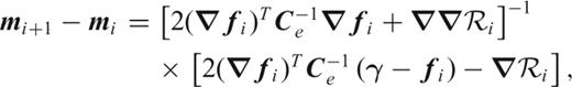
where the subscript ‘i’ stands for the functions evaluated at the ith model iterate. To obtain an reasonable model the conventional approach is to have a misfit to the data of order unity. As our problem relies on two damping parameters, a wide family of (λ_S, λ_T) can satisfy this demand. Moreover, the statement is reliable only if both correlation in the errors and error estimates are perfectly represented; unfortunately this is not the case for the geomagnetic problem. For instance anisotropy in the error treatments as well as correlation between errors could be taken into account (Holme & Jackson 1997; Rygaard-Hjalsted 1997). Furthermore, a model m will in practise not simultaneously satisfy the collection of conditions for all the subsets of data γ_k, of size N_k. For example, we find that our treatment of the survey data globally overestimates the errors, and tends to produce a global misfit for this set that is weaker than unity. Finally, for all the models presented here, we reject all data further than 3 standard deviations (as measured by the estimated error) from the model, except when considering observatory annual means for which manual rejection was previously applied (Bloxham 1989; Jackson 2000). A consequence of this model-dependent data rejection is that all the models reported do not rely exactly on precisely the same number of data.

3.2 Quadratic regularization

The regularization functions and used in geomagnetic field modelling are typically quadratic measures. Spatial norms such as (Shure 1985; Constable 1993), or the minimum ohmic heating norm (Gubbins 1975; Bloxham & Jackson 1989; Jackson 2000) have been widely used. In this paper we employ the norm of Shure (1982),

5

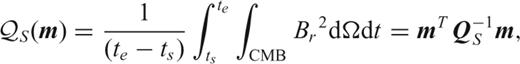
where the integral is defined over a sphere of unit radius. Regarding the temporal regularization function, many time-dependent, spline-based field models (e.g. Bloxham & Jackson 1992; Jackson 2000) have been built using the secular acceleration norm . Sabaka (2004), in their comprehensive model CM4, used instead the secular variation norm , added to a secondary norm in order to regularize the field of internal origin, where and . In this study we use the a similar secular variation norm

6

to implement quadratic temporal regularization. We note that for the quadratic norms (5) and (6), the Hessian and gradient operators of the regularization function appearing in the solver scheme (4) take the form .

We choose the damping parameters (λ_S, λ_T) in order to achieve a balance between the spatial and temporal smoothness, while still satisfactorily fitting the data. Of particular importance in this regard is the sensitivity of model behaviour to the boundary conditions implemented at the endpoints. Because of the lack of information at the extremities of the time span, a relatively strong temporal damping will usually imply that the temporal norm tends towards zero at t_s and t_e. A natural consequence of our scheme (4), where we find a model that minimizes (3), is that the spatial norm can become very large, especially at t_s where there is a much weaker constraint from the data. To help avoid such undesirable effects we strictly imposed the boundary conditions (note that this does not force the temporal norm to be zero).

We choose λ_S by producing a time-dependent quadratic inversion with spatial norm in 1980 similar to that of a 1980 snapshot model, built separately from the Magsat data set (this is the data set which has best coverage and is least noisy). This procedure suggested setting λ_S= 10⁻¹⁰ (in nT⁻² throughout the paper). We then found that taking λ_T= 5 × 10⁻⁶ (in (nT/yr)⁻² throughout the paper) provided a reasonable balance between the temporal and the spatial regularizations. Models were checked to ensure that neither the temporal or spatial norms strongly diverge close to the endpoints. We also note that our results do not depend on the number of splines used. The damping parameters are kept fixed at λ_S= 10⁻¹⁰ nT⁻² and λ_T= 5 × 10⁻⁶ (nT/yr)⁻² throughout the paper, for both quadratic and maximum entropy regularized models.

3.3 Maximum entropy regularization

In this paper we investigate using the entropy of the radial magnetic field image at the CMB as a spatial norm and the entropy of the radial secular variation image at the CMB as a temporal norm, rather than the traditional quadratic norms discussed in the previous section. Skilling (1988) defines the entropy S of a positive function H, over a domain Ω, as

7

where d is a measure which can be interpreted as the default model obtained in the absence of any constraints (the so-called ‘flat map’). From (7) it is possible to define the entropy for functions H consisting of both positive and negative values (Gull & Skilling 1990; Hobson & Lasenby 1998):

8

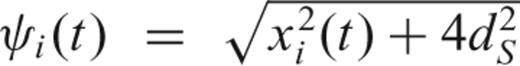
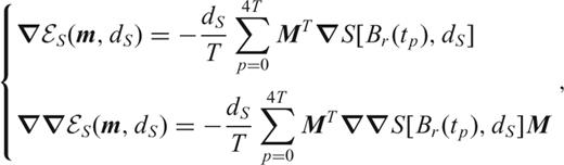
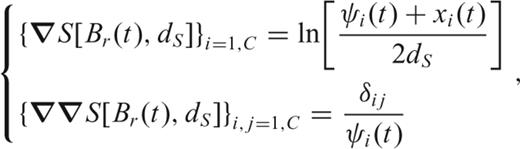
where (see also eq. 12 of Paper I). When looking at the limit of S[H, d] as d becomes very large compared to the typical amplitude of H, a second order Taylor series expansion of (8) gives (e.g. Maisinger 2004)

9

It is therefore, possible to quantitatively benchmark the maximum entropy regularization at large d against quadratic regularized inversions based on the integral of H².

Since the radial magnetic field image at the CMB is not a positive distribution, eq. (8) was used by Jackson (2003) to produce single epoch models using the maximum entropy method. Here, for the time-dependent problem, we take a slightly different approach and begin by writing the spatial norm based on the entropy definition (8) as

10

where d_S is the default parameter associated with the spatial entropy norm. Note d_S has the same dimensions as B_r, so that and also have the same dimension. The −4d_S factor in eq. (10) allows us to take advantage of (9), to have a directly comparable damping parameter for both the quadratic and entropy regularizations. Next we discretize the CMB into a spherical triangle tessellation (STT, see Constable 1993) so the entropy function in (10) becomes,

11

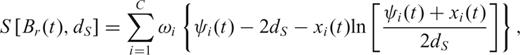
where and x_i(t) =B_r(c, θ_i, φ_i, t) is the radial magnetic field evaluated at the centre of the cell i of surface area ω_i. C= 6480 cells relying on 3242 nodes were used and some more expensive computations with 5762 nodes (11 520 cells) were carried out to verify that convergence as function of the STT grid had occurred. The time span [t_s, t_e] is discretized over 4T equally spaced intervals to numerically perform the temporal integration (10).

Then, using (1) and (2), the vector x(t) ={x_i(t)}_i=1,C, which contains the radial magnetic field values in the cells, can be written as a linear function of the spherical harmonic coefficients:

12

The linear operator M(t), of size C×P, is calculated from the spherical harmonic evaluated on each cell, and the B-spline functions evaluated at the time t (see Appendix A). From (10), (11) and (12) we derive the gradient and Hessian functions in the spectral domain, which we need to perform the iterative process (4):

13

with t_p=t_s+p(t_e−t_s)/4T. The gradient and Hessian functions of S[B_r(t), d_S] in the physical domain are given by Hobson & Lasenby (1998 and Paper I, eqs 13–14):

14

where δ_ij is the Kronecker's symbol.

In a similar manner to eq. (10) we define a temporal norm based on the entropy of the radial secular variation image at the CMB,

15

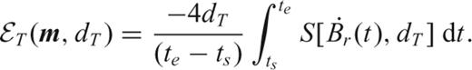
The associated gradient and Hessian functions are computed in the same manner as in (13) and (14), but replacing B_r by and d_S by d_T. The default parameter d_T associated with the temporal entropy norm has the same dimensions as , so that and have the same dimensions.

Note that Jackson (2003) described the entropy constraint in the physical domain (r, θ, φ). Here the decomposition (12) allows us to impose the maximum entropy constraint in the spectral (spherical harmonic) domain in a similar manner as the quadratic constraints were previously implemented. The entropy method also requires an iterative approach using eq. (4), but in comparison with a quadratic inversion, it requires a larger number of iterations to converge. Consequently, we do not estimate the Hessian—the most time demanding step—at every iteration when carrying out a maximum entropy inversion. In practise, we find that convergence is straightforward for relatively large values of the default parameters, but that it is more challenging for smaller values of d_T and d_S, when it also becomes necessary to recompute the Hessian more frequently. We imposed a criterion that the norms presented in Table 2 be converged up to the third decimal place.

2

Values of the misfit , the number of data N, the spatial norms and (in mT²), the temporal norm and [in (μT yr⁻¹)²], and the integrals (in mT) and (in nT yr⁻¹) for several values of the default parameters d_S and d_T. In all cases the damping parameters are fixed at λ_S= 10⁻¹⁰ nT⁻² and λ_T= 5 × 10⁻⁶ (nT/yr)⁻².

Open in new tabDownload slide

We note that the particular choice of the spatial and temporal entropy-based norm remains arbitrary, in a similar manner to how the choice of a particular quadratic norm was arbitrary. In the regularization procedure one could equally well use the entropy of any scalar function of B_r (involving any spatial or temporal derivatives) to construct the norms and . If one wishes to image a particular function of φ(B_r), then the corresponding entropy function S[φ(B_r), d] should be used to penalize the inversion. We have chosen here φ_S(B_r) =B_r for the spatial regularization and for the temporal regularization because this is the most straightforward and easily understood scenario. Note as well that for the core motions problem (Bloxham & Jackson 1991) one needs both B_r and , so that it seems sensible to regularize the entropy function of each of these.

4 MAXIMUM ENTROPY VERSUS QUADRATIC MODELS

4.1 Comparison between quadratic and maximum entropy spatial regularizations

We present in this section the effect of using, instead of a quadratic spatial regularization, maximum entropy regularization in space. The temporal regularization is kept the same (quadratic, i.e. very large default value d_T) throughout this section. We reiterate here that the damping parameters are kept fixed at λ_S= 10⁻¹⁰ nT⁻² and λ_T= 5.10⁻⁶ (nT/yr)⁻² throughout this study.

In Table 2 we present the values of the different norms for all the models we computed. We focus in this section on the upper part of this table, where we test the effect of varying the spatial default parameter d_S. We checked that for large values of this parameter (e.g. here d_S= 10⁴ μT) the norms, misfit and number of data accepted converge towards the values obtained in the quadratic case (cf. Fig. 2 and Table 2). This constitutes a benchmark of our time-dependent spectral domain maximum entropy method against the previously used quadratic method. The convergence at large d_S of the magnetic field models spectra (Fig. 3a) also illustrates this point: when d_S≥ 10⁶ nT all the curves converge towards the quadratic spectrum.

Figure 2

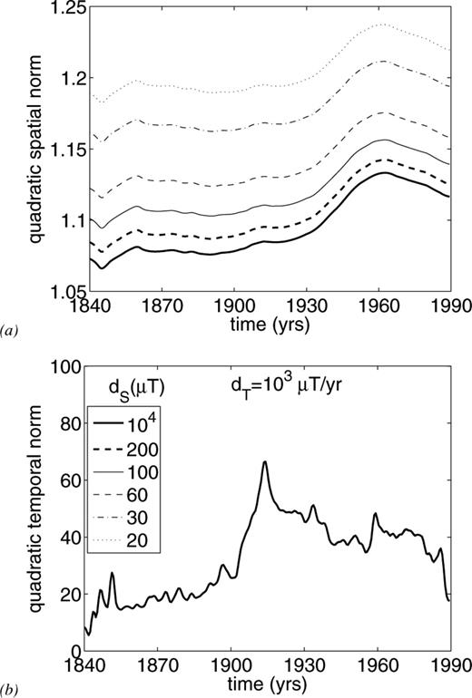
(a) quadratic spatial norm (in mT²) and (b) quadratic temporal norm (in (μ T yr⁻¹)²) for d_T= 10³ μT yr⁻¹ and several values of d_S. The quadratic spatial norm is increasing with decreasing d_S. The evolution of the quadratic temporal norms is very similar in all cases, so cannot be distinguished.

Open in new tabDownload slide

Figure 3

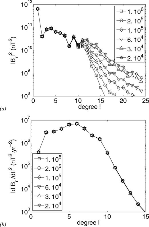
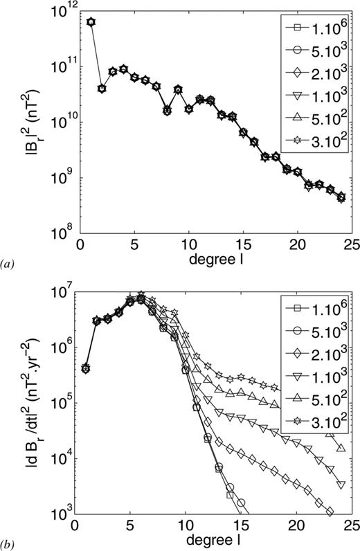
Power spectrum for (a) B_r and (b) for d_T= 10⁶ nT yr⁻¹ and several values of d_S (in nT). When d_S≥ 10⁶ nT the spectra converge towards the quadratic case. The spectra for all coincide, so cannot be distinguished.

Open in new tabDownload slide

Decreasing the spatial default parameter d_S has several implications when looking at the norms: decreases and increases while the temporal norms and are almost unaffected. We checked in Fig. 2 that no time-dependent bias appears when looking at the temporal evolution of the norms. The only modification is an expected upward shift of the spatial quadratic norm (Fig. 2a), while the temporal quadratic norm remains unaffected (Fig. 2b). It is also interesting to note that the time averaged unsigned flux over the CMB,

16

remains almost unchanged between the quadratic and the maximum entropy models (see Table 2). This is a good illustration of the meaning of maximizing the entropy. The fact is not affected too much as d_S is changed tells us that the maximum entropy method is a way of reorganizing a nearly constant amount of magnetic field lines going in and out of the core. This is done in such a way that maxima are raised and minima are depressed—which also increases . It is a completely different process than decreasing the damping parameter λ_S which would also result in an increase in . Decreasing λ_S on the other hand leads to a decrease of the misfit to the data , that is, to undesirable overfitting. That is not the case when using the maximum entropy in space, as shown in Table 2 where both the misfit and the number of accepted data remain similar regardless of the value of d_S. One can check in Table 3 (upper part) that no strong bias has been introduced when modelling the individual data sets.

3

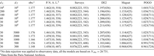
Values of the misfit (with in parenthesis the associated number of accepted data ) of the different subsets of data, for models built with several values of the default parameters d_S (in μT) and d_T (in nT yr⁻¹). In all cases the damping parameters are λ_S= 10⁻¹⁰ and λ_T= 5 × 10⁻⁶.

Open in new tabDownload slide

Another way to evaluate the success of the different regularization methods is to look at the comparison between model predictions and first differences of observatory annual means, as presented in Fig. 4. Both the model built using quadratic spatial regularization (large default value d_S= 10⁴ μT, black) and that built using maximum entropy spatial regularization (low default value d_S= 30 μT, blue) have similar fit to the data. The two model predictions also agree precisely at the two example observatories Niemegk (Germany, Fig. 4a) and Hermanus (South Africa, Fig. 4b). These examples were chosen to illustrate a geographical region where models are tightly constrained by the presence of data from a large number of observatories (in western to central Europe) and a more isolated region in the southern hemisphere (South Africa).

Figure 4

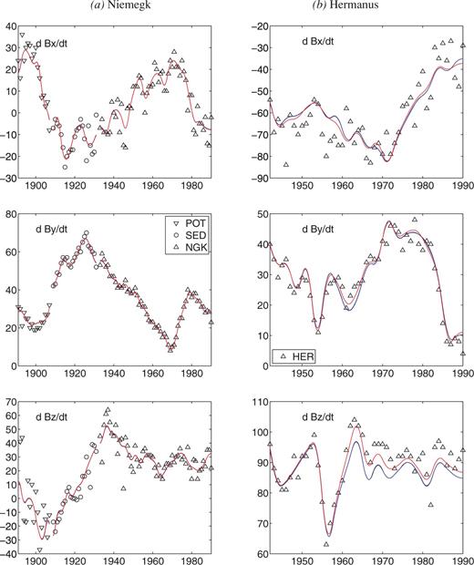
Time series of the time derivative of three components of the magnetic field for (a) Niemegk (NGK) in Germany, together with the near-by observatories SED and POT, and (b) Hermanus (HER) in South Africa. Comparison between the first differences of observatory annual means (open symbols) and the predictions for several models: quadratic in space and time (d_S= 10⁴ μT and d_T= 10⁶ nT yr⁻¹, black curve), quadratic in time and maximum entropy in space (d_S= 30 μT and d_T= 10⁶ nT yr⁻¹, blue curve), and maximum entropy in space and time (d_S= 30 μT and d_T= 300 nT yr⁻¹, red curve). At Niemegk the black and blue curves are nearly invisible as it coincides almost exactly with the red curve. At Hermanus the black curve only is invisible, superimposed with the blue curve. Note on (a) that we have chosen to show three distinct model predictions for the observatories POT, SED and NGK (these result in discontinuities at the transition from POT to SED and from SED to NGK).

Open in new tabDownload slide

Despite the similarity in their statistics the models with d_S= 10⁴ and 30 μT are rather different when snapshots of the field at the CMB are considered, as is presented in Fig. 5. For an equivalent fit to the data the maximum entropy method provides a significantly more contrasted picture of the field, showing a larger number of distinct flux patches (compare Figs 5a–b). At the same time the spectra of B_r at the CMB become more and more flat as d_S decreases (Fig. 3a), whereas the secular variation spectra remains unchanged (Fig. 3b). Care must be taken when interpreting these results: the maximum entropy method does not produce images containing very small length-scale features such as those produced when damping parameters are decreased. Instead it feeds the spectrum of the images at small and intermediate lengthscales in such a way that the large-scale features of the magnetic field become sharper. Of particular interest is the fact that for all the models the spectra are similar for spherical harmonics degrees up to l≃ 10. That gives a measure of the typical minimum size of features that our inversions can unambiguously detect, given the data sets (and their inherent errors) that we have considered.

Figure 5

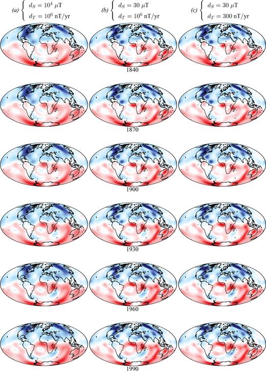
Radial magnetic field at the CMB for six equally spaced epochs from 1840 (top) to 1990 (bottom), for models built using (a) quadratic regularizations in space and time, (b) a quadratic temporal regularization together with a maximum entropy spatial regularization, and (c) maximum entropy regularizations in space and time. For all the snapshots the colourbar ranges from −1 mT (dark blue) to +1 mT (dark red), with contours every 50 μT.

Open in new tabDownload slide

When looking at snapshots of the field at the CMB, we see that the spatial maximum entropy regularization (Fig. 5b) reveals several features that were previously obscured in the quadratic model (Fig. 5a). The blue flux patch over the Northern America is now split into a series of four different patches, present throughout the 1840–1990 interval, and which stretch from under Alaska to under the western Atlantic Ocean near Brazil. We also isolate, under northern tropical latitude and between western Siberia and central Africa, four blue patches that can be associated with the same number of red patches under the equatorial region. The two main red patches in the southern hemisphere under mid-latitudes also show a structure more elongated in the meridional direction, with perhaps the presence of several extrema.

4.2 Comparison between quadratic and maximum entropy temporal regularizations

We present in this section a comparison between a model constructed in Section 4.1 (quadratic temporal norm , maximum entropy spatial norm with d_S= 30 μT) and models built using a maximum entropy norm for the temporal regularization. The spatial regularization is kept the same throughout Section 4.2. The norms and statistics relevant to this section are presented in the lower part of Table 2.

First, we verify that in the case where the temporal default parameter is very large (d_T= 10⁶ nT yr⁻¹) that the use of the maximum entropy temporal norm gives a result similar to that when is used. This constitutes a benchmark of the method. Then by decreasing d_T one can see that decreases, as increases. It is worth noticing the spatial norms and are almost unchanged. This behaviour is in accordance with our expectations, since it is equivalent to what we observed in Section 4.1 when implementing the spatial maximum entropy regularization and keeping the temporal regularization fixed. We check in Fig. 6 that no spurious time-dependent effects appear in the evolution of the norms. The main modification is an upward shift of the temporal norm (Fig. 6b) while the spatial norm remains rather unaffected (Fig. 6a).

Figure 6

(a) Quadratic spatial norm (in mT²) and (b) quadratic temporal norm [in (μT yr⁻¹)²] for d_S= 30 μT and several values of d_T. The quadratic temporal norm is increasing with decreasing d_T. The evolution of the six quadratic spatial norms is almost identical. To help the comparison, the vertical ranges have been chosen similar to those of Fig. 2.

Open in new tabDownload slide

As d_T is reduced the spatial spectrum is not affected, as shown in Fig. 7(a). Instead, the secular variation spectrum is enhanced at large wavenumbers (Fig. 7b) in order that secular variation features with larger spatial gradients (but not with shorter timescales) can be observed. One can see that given our data set, the largest spherical harmonic degree of secular variation that our modelling can unambiguously retrieve is around 6 or 7. We do not yet understand why the spectrum takes the peculiar form involving an inflexion in the tail.

Figure 7

Spectrum for (a) B_r and (b) for d_S= 30 μT and several values of d_T (in nT yr⁻¹). When d_T≫ 10⁴ nT yr⁻¹ all the curves converge towards the quadratic spectrum. The spectra for B_r almost coincide the one with the other.

Open in new tabDownload slide

The integral of the absolute value of the secular variation over the CMB averaged over the time span,

17

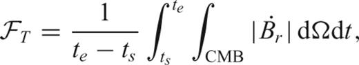
decreases slightly as d_T decreases (see Table 2). However, the amplitude of its evolution is minor compared to those found for the other norms and . In this regard the maximum entropy method can still to a reasonable approximation be interpreted as the rearrangement of the distribution, in order to produce a secular variation picture of higher contrast. It seems the stability of the norms and , noted when decreasing the spatial default parameter d_S in Section 4.1, is stronger than the stability of the norms and observed when decreasing instead the temporal default parameter d_T. This may be an indication that a smaller knot spacing is required as the temporal default parameter is reduced, which requires that sharper temporal changes be modelled.

We have seen that analogies can be drawn between the application of the maximum entropy method to temporal regularization and its use in spatial regularization. There nevertheless exists an essential difference between using the maximum entropy for the spatial and temporal regularizations: one can check in Table 2 that the misfit to the data is slightly reduced as d_T decreases, and also that a larger number of data are accepted. One can see in Table 3 that all the different data sets follow this trend, with the satellite and survey data misfits the most affected. However, this improved fit is not linked to a more complex temporal evolution of the norms, as would happen if we decreased the temporal damping parameter λ_T. Instead, for a given damping parameter, the entropy based temporal regularization allows us to model sharper changes in , without introducing fluctuations on shorter timescales.

This point is illustrated in Fig. 4, where the fit of our models to first differences of observatory annual means (a measure of secular variation) is presented. At Niemegk we can see that all the models give exactly the same prediction, regardless of the value of d_T (Fig. 4a). Note that this time series goes back to around 1890, so that our interpretation about the fit still holds for older data. On the contrary, at Hermanus, the fit to the data improves as the temporal default parameter is reduced (Fig. 4b). We interpret these results as follows: the Niemegk observatory is situated in a very well sampled area (Central Europe) where the data constraint is strong. There are thus very few changes that can be made to the model predictions, without greatly increasing the misfit. On the contrary, Hermanus lies in South Africa where fewer observatories are located, so that the secular variation is much less tightly constrained. Here, the maximum entropy temporal regularization allows us to take into account large changes in the secular variation (especially in the 1960's) without having to decrease the damping parameter λ_T, thus avoiding globally overfitting the data. Note also that for a specific observatory data series, the better the quality of the data, the smaller are the differences in the predictions made by the models built using the and norms.

When looking at the field snapshots in Fig. 5, the global picture seems to be mostly unchanged by the introduction of the temporal maximum entropy regularization—compare the model built with d_T= 10⁶ nT yr⁻¹ (quadratic temporal norm, Fig. 5b) with the one built with d_T= 300 nT yr⁻¹ (maximum entropy temporal norm, Fig. 5c). This reflects the fact that the spectrum of B_r is not affected, so the same power is devoted to the small lengthscales in each case (Fig. 7a). However, when looking more carefully at animations of the field evolution, one can detect some important changes. The most striking is related to the field evolution south of Madagascar, where the birth of a reverse flux patch occurs much later when temporal maximum entropy regularization is employed. One has to wait until the early 20th century for the reverse flux patch to appear, whereas it is already present in 1840 in the models derived using quadratic temporal regularization, regardless of the spatial regularization.

This example is characteristic of one of the effects of maximum entropy temporal regularization: it is capable of modelling sharper temporal changes when needed, as was previously illustrated in the comparison between model predictions and data at the Hermanus observatory (Fig. 4b). Few data are available around the south-west Indian Ocean in the early stages of the studied time span. The use of the quadratic temporal regularization tends to smear back in time the presence of the reverse flux patch that is actually only constrained by data from the first half of the 20th century. For any specific epoch, the use of entropy as a temporal norm allows one to produce time-dependent models without introducing temporal correlation from one epoch to the other, unless the data require it. In a sense it encapsulates the best qualities of snapshot models (e.g. Bloxham 1989) and of time-dependent models (e.g. Bloxham & Jackson 1992).

5 DISCUSSION

In this paper, we have proposed a new regularization method for modelling the time-dependent magnetic field at the CMB, based on maximizing the entropy of non-positive images. We introduced this technique into the inversion process, and applied it to historical data spanning the interval 1840–1990. Entropy norms have been introduced for both the temporal and spatial regularization methods, and comparisons have been carried out with more traditional quadratic regularizations.

By applying the maximum entropy method to the spatial norm, the spectrum of B_r is enhanced at small-to-intermediate lengthscales, in a manner that produces sharper large-scale field features. An image of the radial field at the CMB with improved contrast is obtained without altering the characteristics of the temporal evolution. The fit to the data obtained, as well as the unsigned flux through the CMB, are unchanged compared to the values found for an inversion using quadratic regularization. For the same balance between the misfit to the data and the damping our method provides an alternative way to organize the radial field lines, enabling sharp images of the field to be obtained and making fewer a priori assumptions about the structure of the field. Some new features become apparent (e.g. above North America or Siberia previously broad patches split into several smaller ones) and some previously known features are observed more clearly (e.g. wave-like structures at low latitudes).

Applying the maximum entropy method to the temporal norm, the spatial characteristics remain largely unaffected and the spectrum of B_r is unchanged. We are able to capture sharper temporal variations (those associated with larger spatial gradients in the secular variation) but emphasize that this method cannot capture shorter timescale fluctuations than those captured by conventional quadratic regularization. As a consequences data can locally be better fit in some areas where the geographical constraint on the field morphology is not so strong (e.g. around South Africa). The fit remains similar where the sampling is good, even going back to the 19th century where the data coverage is not so dense (e.g. Western Europe). The technique can, therefore, locally reduce the misfit to the data, but also avoids the smearing back in time of features in the models that are not constrained by the data. The most striking example of this is the reverse flux patch below Madagascar, that appears only after 1900 when maximum entropy temporal regularization is used, whereas it is smeared back to 1840 when a quadratic regularization is employed. In this regard a problem of previous time-dependent models in creating spurious temporal correlations between nearby epochs is avoided.

The method has been tested here on 150 yr of geomagnetic observations; in the future we plan to extend its application to the complete historical data set used by Jackson (2000), together with more recent data spanning the past 15 yr. Improved tests concerning the existence of the westward drift wave-like patterns (Finlay & Jackson 2003) and for their dispersion (Finlay 2005) will then be carried out. The maximum entropy method could also be used to build a new archeomagnetic field model, and help avoid artificial correlations being introduced where gaps in the data are present in both space and time, especially in the southern hemisphere (Korte & Constable 2005; Korte 2005). It would be interesting to test such models for the presence of both westward and eastward motions of the magnetic flux patches on the millennium timescales (Dumberry & Finlay 2006). In addition, one could apply our method to both core and crustal fields in comprehensive models, or in focused lithospheric field modelling. This could perhaps help push further, in terms of spherical harmonic degree, the limit of the robust modelling of the main field (Sabaka 2004; Sabaka & Olsen 2006; Maus 2007).

The construction of maximum entropy models of the radial magnetic field and its secular variation is also promising from the perspective of obtaining more accurate models for the motions u at the surface of the core, through the radial component of the induction equation

18

where ∇_h=c⁻¹[0, ∂_θ, (sin θ)⁻¹∂_φ] is the horizontal gradient operator, and D_r is the radial component of the magnetic field diffusion operator. To reconstruct the velocity field workers often make the assumption that diffusion is negligible, the so-called frozen flux approximation (Roberts & Scott 1965). In addition a second constraint on the flow dynamics is also made—for example, steady, tangentially geostrophic, toroidal motions, etc. (Bloxham & Jackson 1991). One can see from (18) that the inverse problem for the flow does depend on the horizontal gradients in B_r. Thus sharper models of B_r obtained with a maximum entropy regularization (capturing larger horizontal gradients) may improve the resolution of core flow features such as polar vortices (Eymin & Hulot 2005). Maximum entropy regularized field models may also contain smaller regions enclosed by iso-contours of B_r/cos(θ) not reaching the equator. These so-called ‘ambiguous patches’ are regions where the flow is non-unique under the widely employed tangentially geostrophic approximation (Le Mouël 1984).

The frozen flux constraint implies that the magnetic field flux is conserved inside null-flux curves (Backus 1968). It has been shown that it is possible to build magnetic field models that satisfy this constraint (Constable 1993; O'Brien 1998; Jackson et al., submitted). Rau (2000) also suggested that the frozen flux approximation may be reasonable based on studies of some geodynamo numerical simulations. However, the data constraints still permit considerable freedom in the model parameters, and the presence of diffusive processes cannot be ruled out (Bloxham & Gubbins 1985). For example, some features required by the data, such as the birth of a reverse flux patch under Madagascar, cannot be easily accounted for within the framework of the frozen flux hypothesis. Mechanisms involving magnetic diffusion, such as expulsion of toroidal field by up-welling flow, must be invoked (Gubbins 1996). The maximum entropy method employed here has the interesting property of clarifying the topology of the radial field map. This should allow more accurate tests of the magnetic flux changes through null-flux curves and therefore better tests the validity of the frozen flux approximation, and its impact on the ability of field models to satisfactorily explain observations.

ACKNOWLEDGMENTS

The authors thank Richard Holme for providing the idea of implementing the maximum entropy regularization in spherical harmonics. NG was supported by a NERC postdoctoral fellowship (grant number NER/A/S/2003/00451). CF was supported by a NERC postdoctoral fellowship, as part of the GEOSPACE consortium (grant number NER/O/S/2003/00674). This is Institüt für Geophysik contribution no. 1506.

APPENDIX A: CONVERTION FROM SPHERICAL HARMONICS TO STT

The magnetic field x_i(t) =B_r(c, θ_i, φ_i, t) can be written from (1) on any cell i as

(A1)

where ϕ(l) = (l+ 1) (a/c)^l+2. Using the B-spline basis defined in eq. (2) for the temporal representation, one can show that

(A2)

From (A2) one can write the magnetic field x_i(t) at any given cell and time as

(A3)

where m_k is the kth component of the spherical harmonic model. Each element of the matrix M(t) is given by

(A4)

REFERENCES