A covariance-adaptive approach for regularized inversion in linear models Free

Summary

1 Introduction

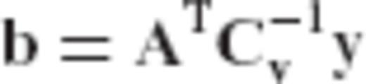
A generic estimation problem in many geodetic and geophysical applications is that of determining a set of unknown deterministic parameters which are observed through a known transformation model and corrupted by additive random noise. This type of problem is commonly formulated in terms of a linear system of observation equations , which needs to be uniquely solved for the unknown parameter vector x given a set of noisy data y (Tarantola 1987; Menke 1989; Dermanis & Rummel 2000). The residual term v describes the effect of random disturbances in the input data, whereas the elements of the matrix A correspond to known coefficients that depend on the conditions of the physical system under study. Note that such problems are inherently ill-posed as they can never have a unique solution due to the existence of the unknown random observation errors. In algebraic terms, we deal with an underdetermined system that has an infinite number of solutions, since for every candidate solution for the parameter vector there always exists a corresponding estimate of the unknown data errors, , which satisfies the original system of observation equations.

Typical examples of such discrete inverse problems arise in several fields of geosciences, including gravity field modelling and satellite geodesy (Schwarz 1979; Rummel 1985; Sanso & Rummel 1989; Xu 1992; Xu & Rummel 1994; Ilk et al. 2002), satellite orbit determination (Engelis & Knudsen 1989; Beutler et al. 1994; Tapley et al. 2004), tectonic plate motions (Chase & Stuart 1972; Minster et al. 1974), satellite altimetry and ocean circulation studies (Wunsch & Minster 1982; Knudsen 1992; Fu & Cazenave 2001), magnetic field modelling (Parker et al. 1987; Backus 1988), atmospheric tomography (Kunitake 1996; Kleijer 2004), seismology and acoustic tomography (Crosson 1976; Aki & Richards 1980; Pavlis & Booker 1980), wave propagation and scattering theory (Bee & Jacobson 1984; Koch 1985) and core and mantle dynamics (Parker 1970; Gire et al. 1986; Nataf et al. 1986).

A fairly common approach for solving parameter estimation problems in linear models is the method of least-squares (LS) which provides an optimal solution that reproduces as close as possible the given data by minimizing the weighted differences between the original measurements y and the model-induced observables . In statistical terms, the LS solution gives an unbiased estimate for the unknown parameters provided that there are no modelling errors or other hidden systematic effects in the data. In addition, it has the minimum mean squared estimation error (MSEE) among all linear unbiased estimators if the chosen weight matrix for the input data is equal to the inverse covariance (CV) matrix of their random observation errors; for more details, see Menke (1989), Koch (1999) and Rao & Toutenburg (1999).

Within the context of geodetic and geophysical applications, the LS methodology has been used not only as an optimal algorithm for estimating a set of unknown parameters from noisy measurements in a given linear model, but also as a trend analysis tool for identifying the main features of partially known physical systems through the fitting of simple analytic models to complex data records. In any case, the accuracy of LS inversion results may not be satisfactory in practice if the underlying linear model that relates the available data and the unknown parameters is ill-conditioned. In such cases, one or more eigenvalues of the corresponding normal matrix are close to zero, thus causing a large statistical uncertainty in the LS solution even for very precise data sets (Hoerl & Kennard 1970; Sen & Srivastava 1990). In this category belong many geodetic estimation problems that can be expressed in the linear form y = Ax+v, including the downward continuation of gravity field measurements from satellite or aerial altitude to the surface of the earth, the inversion of altimetric data for marine gravity determination, and the computation of gravity gradients from gravity anomaly data. For a general overview of ill-posed inverse problems in geodesy, see Neyman (1985) and Ilk (1991).

Various alternative techniques to the classic LS method have been developed in order to improve the parameter estimation accuracy in linear model inversion. Despite their differences and (sometimes) conflicting interpretations, most of these regularization techniques seem to follow a common rationale which points to the fact that a successful solution to a discrete inverse problem should not be solely determined by the quality of the fit between the data and the corresponding observables obtained from the estimated model parameters (i.e. the typical ‘LS logic’), but it requires also some quality control for the estimated parameters themselves. As an example, we can mention the method of Tikhonov—Philips regularization (Tikhonov & Arsenin 1977) which has been used extensively for the stable inversion of ill-conditioned linear models based on a hybrid optimal criterion that takes into account both the data-model fitting aspect and the size or smoothness of the actual model parameters (Schwarz 1979; Schaffrin 1980; Ilk et al. 2002; Kusche & Klees 2002; Ditmar et al. 2003). Other perspectives of the Tikhonov—Philips inversion scheme have also been considered by many researchers, including its implementation from a biased estimation or ridge regression viewpoint (Xu 1992; Xu & Rummel 1994; Bouman & Koop 1997), and its Bayesian interpretation which involves a priori parameter weighting (Xu & Rummel 1994) and variance component estimation procedures (Koch & Kusche 2002). Alternative regularization approaches that have been followed for the optimal inversion of linear models include the truncated singular value decomposition (TSVD) or bandpass filtering (Xu 1998), stochastic regularization techniques (Schaffrin 1985, 1989), LS collocation (Rummel et al. 1976, 1979) and numerical iterative methods (Landweber algorithm, conjugate gradient algorithm). A detailed comparison of regularization techniques for geodetic inverse problems has been given in Bouman (1998), where a unified framework for the spectral behaviour of several regularized estimators was presented; see also Gerstl & Rummel (1981).

The objective of this paper is to present a new parameter estimator for linear models y = Ax+v, which unifies under a common statistical framework all regularization methods that are systematically used in geodetic inverse problems. Our study lies on the fact that it adds an alternative perspective on the optimal statistical properties and the regularization mechanism of many inversion techniques commonly used in geodesy and geophysics, including Tikhonov—Philips regularization, generalized ridge regression (GRR) and TSVD estimation. The structure of the paper is organized as follows. In Section 2, the formulation and the properties of the new parameter estimator are presented along with the derivation of its analytic form. Additional topics of study in this section include the MSEE performance and the inherent bias characteristics of the new estimator, as well as the admissible range for the signal-to-noise ratio (SNR) of an arbitrary linear model that guarantees better MSEE performance when using the new estimator over the classic LS solution. Some particular regularization aspects associated with the new parameter estimator are discussed in Section 3, where it is shown that all regularized inversion techniques corresponding to an eigenvalue filtering of the normal matrix of the underlying linear model y = Ax+v are essentially special cases of the general estimation framework presented herein. An example for the numerical solution of a typical ill-conditioned problem in physical geodesy, namely the downward continuation of satellite gradiometry data for the determination of a gravity anomaly grid on the surface of the Earth, is given in Section 4 to demonstrate the practical implementation and the usefulness of the new estimator in geodetic inverse problems. Finally, some concluding remarks are given at the end of the paper.

2 CV-Adaptive Parameter Estimation in Linear Models

2.1 Problem formulation

Let us consider the standard linear model that is commonly used for tackling discrete inverse problems in geodesy (Xu & Rummel 1994; Xu 1998; Dermanis & Rummel 2000)

1

where y is a known observation vector, A is a matrix of known coefficients whose values depend on the geometrical and physical conditions of the data modelling process and x is a vector of unknown deterministic parameters. The residual term v corresponds to a vector of zero-mean random variables with a CV matrix C_v, and it describes the effect of random errors and other stochastic disturbances in the available data. Although it is not crucial for our problem formulation to specify the exact nature of the observations and the unknowns, it is nevertheless worth mentioning that eq. (1) often corresponds to a discretized Fredholm integral equation of the first kind with noisy data. This type of integral equations provides the fundamental mathematical basis for describing and studying several ill-posed inverse problems in geodesy and geophysics (Neyman 1985; Ilk 1991; Bouman 1998). In gravity field modelling, for example, the system in eq. (1) can describe the problem of marine gravity determination from satellite altimetry data using Hotine's or Stokes' integral, or the downward continuation of satellite and/or aerial gravity field data based on Poisson's integral (Heiskanen & Moritz 1967).

The optimal inversion of eq. (1) will be based on a tailoring methodology, according to which a known reference estimator of x is modified in such a way that it produces an improved solution for the unknown model parameters. This kind of constructive reasoning has actually shaped the development of several parameter estimators in statistics theory (Bibby & Toutenburg 1977). Following Rao (1973), an improved estimator may be heuristically described as one which is derived in the following manner: starting with some prescribed solution, say , having known statistical properties of bias, variance, etc., we try to adapt it in some way so that a newly generated estimator (based on ) is better in terms of some chosen criterion function. For instance, if the criterion function is the MSEE, then we should say that is better than if is smaller than (for more details, see Bibby & Toutenburg 1977).

In this paper, we form an optimal estimator for the parameter vector x in a linear model y = Ax+v based on a linear transformation of the classic LS solution (or equivalently, the minimum-variance linear unbiased solution). Thus, we have the following general scheme

2

with denoting the usual LS estimator

3

and R being a transformation matrix that needs to be determined according to some optimal criteria for the performance of .

Despite its optimal statistical properties, the LS solution in eq. (3) gives poor results when the original linear model is ill-conditioned. The effect of the matrix R in eq. (2) should thus be understood in a ‘regularization’ context as an attempt to correct the LS solution by adjusting it closer to the true vector x. In fact, many well-known regularization techniques are known to produce parameter estimators that can take the form of eq. (2) for specific expressions of the matrix R, including Tikhonov—Philips regularization, GRR, shrunken LS estimation, TSVD estimation and principal component estimation (Marquardt 1970; Mayer & Willke 1973). Note that the numerical implementation of the modified estimator does not necessarily require the prior computation of the entire LS solution (which is actually problematic in the case of ill-conditioned problems), provided that the matrix product R (A^TC⁻¹_vA)⁻¹ can be separately evaluated in a numerically stable and efficient manner (more details given in Section 3).

Our aim is to determine a general form for the regularization matrix R by combining (i) a ‘global’ optimal criterion that minimizes the weighted difference between the original LS solution and the transformed LS solution obtained from eq. (2) and (ii) a constraint that sets the error CV matrix of the modified estimator equal to an a priori, user-specified form.

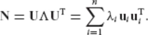
As it will be shown in later sections, all existing regularization methods for discrete inverse problems that correspond to an eigenvalue filtering of the ill-conditioned normal matrix N = A^TC⁻¹_vA can be formulated as special cases of the aforementioned framework. This kind of unification adds an interesting perspective on the statistical properties and the regularization mechanism of many inversion techniques that are currently used in geodesy and geophysics, by interpreting them as a collection of ‘CV-adaptive’ parameter estimators that obey the same optimal criterion and differ only on the pre-selected form of their error CV matrix under a fixed model design.

2.2 CV-adaptive inversion methodology and optimal regularization matrix

A fundamental characteristic of the LS solution is its unbiasedness, under the absence of any modelling errors. From the Gaussian viewpoint of LS estimation theory, the property of unbiasedness is essentially a constraint that is a priori imposed on the first moment of a linear estimator in conjunction with the minimum MSEE principle.

Here we seek an optimal parameter estimator by imposing an a priori constraint on its second (centred) moment . Since the general form of is taken as a linear transform of the LS solution according to eq. (2), a constraint on its second centred moment can be formulated in terms of the matrix equation

4

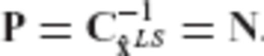
where is the user-specified CV matrix of the estimated parameters, N = A^TC⁻¹_vA is the normal matrix of the underlying linear model, and R is the required transformation matrix.

Note that the CV matrix of the estimated model parameters is identical to the CV matrix of the corresponding estimation errors , since

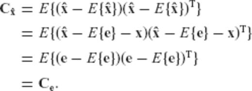
The required regularization matrix R cannot be uniquely determined through the matrix constraint in eq. (4). Hence, apart from its CV-adaptivity, an additional optimal property will be assigned to the estimator in terms of the principle

5

where the weight matrix P is taken as the inverse CV matrix of the LS solution; .

The parameter estimator is thus characterized by two basic statistical properties.

• 1

  It adheres to a minimization criterion that provides an optimal weighted fit with the LS solution according to eq. (5). The particular choice of the weight matrix P as the inverse CV matrix of ensures that the information about the parameter estimation accuracy in the original LS solution is assimilated into the new estimator by adjusting the elements of according to the dispersion of the corresponding elements of .

• 2

  It complies with a user-dependent constraint that specifies the variance and the correlation structure of the parameter estimation errors through an a priori selected CV matrix . Particular strategies and further discussion pertaining to the choice of will be given in Section 3.

From the combination of the above properties we can determine the required regularization matrix R according to an analytic procedure which is described in detail in Appendix A. The final result is given by the following formula:

6

In Appendix B it is proven that the above non-symmetric matrix is also equal to the alternative expression

7

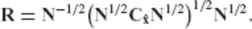
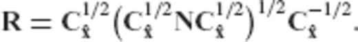
Remark 1: The square root of a symmetric non-negative definite matrix C is a unique matrix which is determined through the square roots of its eigenvalues. In particular, if C = UΛU^T is the orthonormalized eigenvalue decomposition of C, then we have that C^1/2 = UΛ^1/2U^T, where the diagonal matrix Λ^1/2 contains the square roots of the eigenvalues of C. Also, the inverse square root of a symmetric positive definite matrix is defined as (for more details see Rao & Toutenburg 1999, pp. 362–363).

Remark 2: Using the matrix identity ST^1/2S⁻¹ = (STS⁻¹)^1/2, it is easily verified that the optimal regularization matrix can also be expressed through the formula

8

In the trivial case that we choose , the regularization matrix becomes identity (R = I) and our inversion scheme simply reproduces the LS solution, as it should be expected.

2.3 Bias of the CV-adaptive estimator

The CV-adaptive estimator that was introduced in the previous section gives, in general, a biased solution for the unknown model parameters. Its associated bias vector is

9

where R is the regularization matrix obtained from eq. (6) or (7). By making use of the unbiasedness property of the LS solution, the above bias vector can be also expressed as

10

where d denotes the difference between our CV-adaptive estimator and the LS estimator.

Let us now rewrite the minimization principle which was previously introduced for the construction of the regularization matrix R (see eq. 5) in the equivalent form

11

The optimality of the CV-adaptive estimator, in terms of satisfying the above criterion, is closely related to the reduction of its inherent bias. This relationship is more clearly seen through a spectral representation approach, and for this reason let us consider the eigenvalue decomposition of the normal matrix N

12

where U =[u₁ … u_n] is a unitary matrix formed by the orthonormal eigenvectors and Λ = diag(λ₁, …, λ_n) is a diagonal matrix containing the eigenvalues of N. Using the above factorization, the criterion function can be expressed as

13

where n is equal to the number of the unknown parameters (n = dimx).

Also, using eq. (10), the bias vector can be represented in the following spectral form

14

The squared magnitude (Euclidean length) of the above bias vector takes the generalized Pythagorean expression

15

Using the well-known fact that the mean squared value of any random variable is always greater (or equal) than the square of its mean value, we have that

16

Comparing eqs (13) and (16), we can conclude that the minimization of the criterion function is equivalent to a weighted minimization of the maximum bias' Euclidean spectral components, with respect to the orthonormal basis formed by the eigenvectors of the normal matrix N.

Remark 3: The fact that the CV-adaptive estimator is optimized through a fitting to the classic LS solution may be perceived as a ‘weak’ point, due to the problems associated with the LS solution in ill-conditioned problems. However, a closer look at the formulation of the minimization principle in eq. (5) reveals that the fitting does not take place with a particular LS solution, but rather it takes place over the entire ensemble of possible solutions that we would obtain if we repeat the data collection and the LS inversion process an infinite number of times. Moreover, as seen from the previous analysis, the optimality of the CV-adaptive estimator in terms of achieving a best average quadratic fit with the LS estimator is essentially a means to control its inherent bias.

2.4 MSEE performance and admissible SNR range

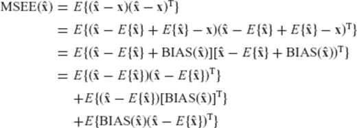
The evaluation of the statistical accuracy of the CV-adaptive estimator requires the analysis of its MSEE matrix

17

The above matrix is usually decomposed into two parts which reflect the additive contributions of the internal precision (variance and correlation structure) and the external accuracy (bias) to the total mean squared error of the estimated parameters. Taking into account the bias expression from eq. (9), we have

18

where is the a priori chosen CV matrix of , and R is the associated regularization matrix obtained from eq. (6) or (7).

We shall consider a scalar measure of the total MSEE of , namely the trace of its MSEE matrix

19

which can be used to quantify the average (per parameter component) MSEE of the entire solution. Note that Q denotes the symmetric matrix

20

which is non-negative definite due to its factorization as a product of a square matrix with its transpose (Harville 1997, p. 213). In this way, the following basic inequality holds (Strang 1988, pp. 348–349)

21

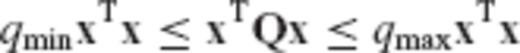
for any parameter vector x. The quantities q_min and q_max correspond to the minimum and maximum eigenvalues of Q, and they depend directly on the regularization matrix R. The maximum eigenvalue q_max, in particular, plays an important role in the assessment of the performance of the CV-adaptive estimator. The quadratic form x^TQx is equal to the squared magnitude of the bias vector , and thus q_max quantifies the maximum relative bias effect in the parameter solution .

Applying the previous inequality into eq. (19), we get

22

Let us now compare the CV-adaptive estimator and the classic LS estimator , in terms of their MSEE performance. Due to its unbiasedness property, the MSEE matrix of the LS estimator is equal to its CV matrix

23

and thus the scalar MSEE takes the simple form

24

In this case, the MSEE of the LS parameter estimator is bounded as follows

25

where λ_min denotes the minimum eigenvalue of the normal matrix N.

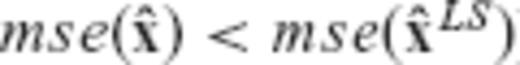
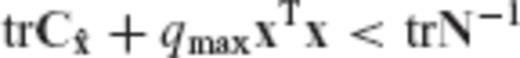
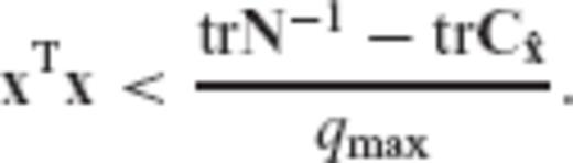
By comparing eqs (22) and (25), we see that the MSEE of the LS estimator has an upper bound that is completely independent of the magnitude of the unknown model parameters, whereas the MSEE of the CV-adaptive estimator has an upper bound that depends directly on the Euclidean length of the parameter vector. Such a result indicates the potential of the biased estimator to produce better results (with significantly smaller MSEE compared to the classic LS solution) in inverse problems with sufficiently low SNR. In fact, an admissible SNR range for an arbitrary linear model can be derived, within which the CV-adaptive estimator is guaranteed to outperform the LS estimator in the MSEE sense.

Let us first define the SNR of a linear model in terms of the ratio

26

The above quantity reflects the average (per parameter component) relative power of the parametric model with respect to the average noise level in its input data.

Taking into account eqs (22) and (24), the following inequality gives a sufficient condition to ensure MSEE improvement in linear model inversion when using the CV-adaptive estimator instead of the LS estimator [i.e. ]

27

or equivalently

28

Using the SNR definition from eq. (26), we finally obtain

29

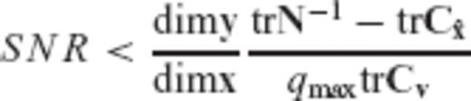
which defines the admissible SNR range for a linear model that justifies the use of the CV-adaptive estimator . The smaller the SNR value of a particular model y = Ax+v with respect to the upper bound given in eq. (29), the greater will be the reduction of the MSEE of .

Note that the quantities dim x, dim y, trN⁻¹ and trC_v are model- and data-dependent, whereas the terms q_max and are controlled by the a priori choice of the CV matrix for the estimated parameters.

As a final comment, we should mention that in every linear model there will always exist an admissible SNR range for applying the CV-adaptive biased estimator, provided that the latter is set to have smaller total error variance than the LS solution. Indeed, in such a case we have that and the right side of the inequality condition (29) will always give a positive upper bound for the admissible SNR of the underlying linear model.

3 Choice of —Regularization Aspects

3.1 General remarks

The a priori choice of the error CV matrix for the estimated parameters is a key issue for the implementation of the CV-adaptive estimator . Although it may seem perplexing to formulate an inversion scheme which conforms to a user-specified error CV structure for the estimated model parameters, the introduction of an external constraint for should be seen as a prospective regularization tool that gives us the flexibility to obtain and compare different solutions for the model parameters with particular statistical quality characteristics.

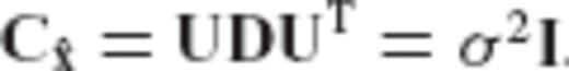
A relevant example is the case where the CV-adaptive estimator is designed to give a fully decorrelated solution with uniform precision for the model parameters, . This particular choice (which is actually equivalent to a special implementation of GRR, as it will be explained later on) can be beneficial in inverse problems y = Ax+v with a large number of unknown parameters that will be subsequently used for the determination of other quantities of interest z = f(x). The existence of a diagonal-scalar CV matrix simplifies to a large extent the accuracy assessment of , at least with respect to the rigorous propagation of random-related errors.

From an algebraic viewpoint, the regularization process in linear model inversion is usually viewed in terms of its filtering effect on the spectral representation of the traditional LS estimator (Gerstl & Rummel 1981; Bouman 1998). The LS inversion of a linear model can be represented through the orthogonal expansion

30

where b denotes the data-dependent vector

31

and {u_i}, {λ_i} are the eigenvectors and eigenvalues of the normal matrix N = A^TC⁻¹_vA

32

In ill-conditioned inverse problems one, or more, of the eigenvalues {λ_i} have very small magnitudes, thus causing problems of numerical instability and significant noise amplification in the LS solution from eq. (30).

In order to overcome these problems and obtain a stable solution with satisfactory accuracy, the classic LS estimator is modified according to the general scheme

33

The role of the filter factors {δ_i} is to stabilize the inversion of the input data, while improving the overall accuracy of the estimated model parameters. The above filtering mechanism provides a common view on various regularization methods in ill-conditioned inverse problems, whose individual characteristics are dictated by the form of their corresponding filter factors. The analytical expressions of {δ_i} for many popular regularization techniques used in geodetic and geophysical inverse problems, including Tikhonov—Philips regularization, GRR, LS collocation, TSVD, Landweber iteration method and conjugate gradient iteration method, can be found in Bouman (1998).

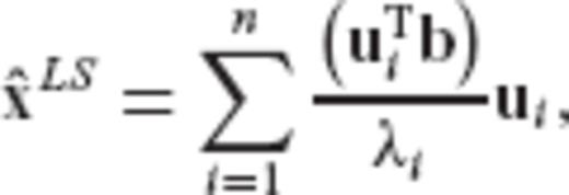
In the next section, it is shown that the CV-adaptive estimator from Section 2 corresponds to an eigenvalue filtering of the type given in eq. (33) for a particular ‘restrictive’ choice of the error CV matrix for the model parameters.

3.2 CV-adaptive regularization in the LS-based eigenvector basis

The problem of selecting the CV matrix of the estimated model parameters for the implementation of the CV-adaptive estimator can be simplified if the choice of is restricted to an a priori general form. Specifically, we adopt the following scheme:

34

where U is the unitary matrix associated with the eigenvalue decomposition of the normal matrix N = A^TC⁻¹_vA (see eq. 32), and D = diag(d₁, …, d_n) is an arbitrary diagonal matrix with non-negative elements. In this way, the CV matrix is constrained to have the same eigenvectors as the normal matrix of the underlying linear model, and its a priori selection is reduced into a problem of specifying only its eigenvalues.

Based on eq. (34), the optimal regularization matrix from eq. (6) or (7) takes the form

35

where Λ is the known eigenvalue matrix of the normal matrix N.

In this case, the auxiliary matrix Q = (R−I)^T (R−I) is

36

and its eigenvalues {q_i} are given by the general analytic formula

37

Furthermore, the CV-adaptive estimator can be expressed in terms of the spectral expansion

38

or equivalently

39

where the data-dependent vector b has been defined in eq. (31).

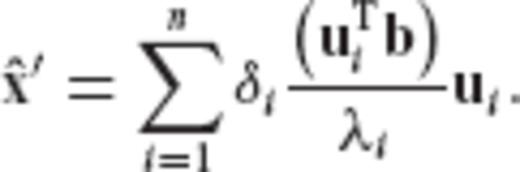
It is seen that the general choice of eq. (34) leads to a CV-adaptive estimator which is equivalent to an eigenvalue filtering of the normal matrix in the underlying linear model. As such, it can cover all regularization techniques that are based on the spectral expansion of eq. (33).

The filter factors {δ_i} associated with the CV-adaptive estimator have the general form

40

and they depend uniquely on the chosen eigenvalues {d_i} for the CV matrix .

By inverting the previous formula, we get

41

which establishes a one-to-one connection between existing regularized estimators that use specific parametrized forms for their filter factors {δ_i}, and the CV-adaptive estimator resulting from the CV-matrix constraint in eq. (34).

A regularization scenario of particular interest within the context of the CV-adaptive estimator is to set all eigenvalues {d_i} equal to the same positive value σ². Such a choice implies an a priori diagonalization constraint for the CV matrix (‘whitening’ of the parameter estimation errors) and it results in a decorrelated solution with uniform precision for the model parameters. It is actually interesting that this type of solution can be equivalently obtained through the well-known method of GRR by properly selecting its built-in regularization parameters. In general, the filter factors associated with the GRR method are given by the formula (Bouman 1998)

42

where {k_i} is a set of regularization parameters that appear in the GRR solution

43

and K = diag(k₁, …, k_n); see Xu & Rummel (1994).

If we set

44

for some chosen positive σ that satisfies for every eigenvalue λ_i of the normal matrix N, then the GRR filter factors from eq. (42) become

45

The equivalent filtering implementation of the CV-adaptive estimator , according to eqs (39) and (40), requires that the eigenvalues {d_i} of should be chosen as

46

which in turn implies the diagonalization constraint .

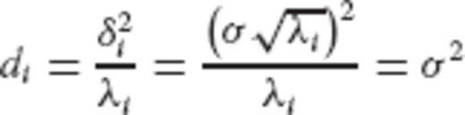
In Table 1, the analytic forms of the filter factors {δ_i}, the corresponding eigenvalues {d_i} of the CV matrix , and the maximum eigenvalue q_max of the auxiliary matrix Q, are provided for some known regularization methods (see also Bouman 1998). Note that all regularized estimators shown in Table 1 can be considered as special cases of the CV-adaptive estimator , for a particular a priori constraint on the CV matrix of the estimated parameters drawn from the general choice .

Table 1.

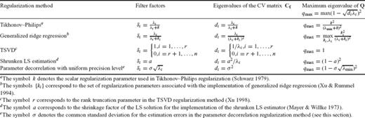
The analytic forms of the filter factors, the eigenvalues of the CV matrix for the estimated model parameters and the maximum eigenvalue of the auxiliary matrix Q, for some common regularization techniques in linear model inversion.

Open in new tabDownload slide

Remark 4: A more general regularization scheme can emerge from the use of the CV-adaptive estimator if the chosen eigenvectors of are different from the eigenvectors of the normal matrix N = A^TC⁻¹_vA. In this case, the optimal approximation of the unknown parameter vector is performed in a different orthogonal basis than the one used in traditional regularization schemes which rely on the eigenvalue filtering with respect to the eigenvector basis associated with the normal matrix N (see Section 3.1). In the context of the present paper, the use of such a different ‘regularization basis’ should be linked to the ability of the CV-adaptive estimator to impose an arbitrary structure on the error variances and covariances of the inversion results. As an example, we can mention the choice with , which gives a decorrelated solution with different error variances for the estimated parameters.

4 Numerical Example

A simulated numerical experiment has been performed to demonstrate the practical implementation and the usefulness of the proposed CV-adaptive regularization scheme. This particular example has been motivated by a similar experiment that is reported in Xu (1998) and it deals with a typical ill-posed inverse problem of downward continuation of gravity field functionals. More specifically, we consider the determination of a gravity anomaly grid on the surface of the Earth using gradiometric observables collected at satellite altitude of 200 km. The basic mathematical model that is used for the design of the experiment is given by the integral equation

47

where T_rr is the second radial derivative of the disturbing potential, R is the mean radius of the Earth, Δg is the gravity anomaly signal, and σ_s denotes the unit sphere. The kernel function S″ (r, ψ) corresponds to the second derivative of the generalized Stokes function with respect to the geocentric radial distance r (for more details, see Xu 1998).

Assuming that we have available n discrete gradiometric observations of T_rr (e.g. via a satellite gravity mission such as GOCE), the integral formula in eq. (47) can be discretized according to the following linear model

48

(see e.g. Xu & Rummel 1995; Xu 1998), where Δg_k are block-mean gravity anomalies, the constant (4πR/10) originates from the generalized Stokes' formula and unit regulation, and Δσ_k and are given by

49

50

51

52

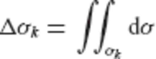
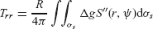
Using the discretized model of eq. (48), a linear system of observation equations can be formed, where y is the data vector with elements , A is the design matrix whose elements correspond to the products , x is the unknown vector of surface block-mean gravity anomalies Δg_k, and v is the data noise vector.

For our experiment, true 1°× 1° block-mean gravity anomaly values have been simulated within an 10°× 10° test area, using the Hirvonen CV function model

53

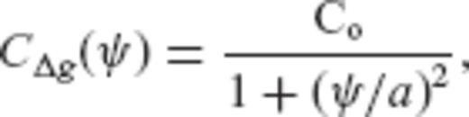
where , and the parameter a has been selected such that the correlation length of the gravity anomaly field is = 15.5 km. The number of satellite gradiometric observables Tⁱ_rr is 400, taken on an 30′× 30′ grid that is located directly above the area of interest at a constant altitude of . The accuracy of Tⁱ_rr is set to 0.01 E(1 E = 10 ⁻⁹ s⁻²), which was also employed in similar simulations by Koop (1993), Xu & Rummel (1995) and Xu (1998). The random errors v for the determination of the synthetic observations from the simulated gravity anomalies are generated according to (4πR/10) N(Tⁱ_rr), where N(Tⁱ_rr) is a Gaussian random number generator with mean zero and variance 10⁻⁴E².

We shall compare two different estimators for the downward continuation of the gradiometric data and the determination of the surface gravity anomaly grid. First, the inversion of the gradiometric measurements is performed using the standard LS methodology, without applying any special regularization tool. The condition number of the normal matrix is 1.93×10⁶, and its eigenvalues range from 1.58×10⁻⁵ to 30.57. As expected, the accuracy of the LS inversion results is considerably poor, giving an average error standard deviation of ±50 mgal in the estimated gravity anomaly values. The detailed statistics of the LS estimation errors are shown in Table 3, where it is seen that extreme errors of more than ±120 mgal occur during the downward continuation of the gradiometric data. In Table 2, we see the statistics of the estimated Δg values which exhibit much stronger variability than the original true values, thus indicating the numerical instability of the downward continuation process through a simple LS inversion algorithm.

Table 3.

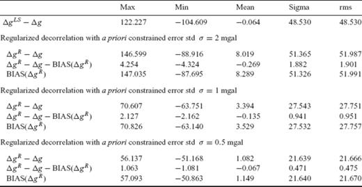
Statistics of the estimation errors in the block-mean gravity anomalies obtained from (i) standard LS inversion of the gradiometric data and (ii) regularized decorrelation for varying values of the a priori constrained error variance. The statistics of the estimation bias in the downward continuation results that are obtained from the regularized decorrelation inversion scheme are also shown. Note that the bias vector for the whole set of the block-mean gravity anomalies is determined as , where x contains the true (simulated) values and R corresponds to the optimal regularization matrix for each a priori choice of σ² (all values in mgal).

Open in new tabDownload slide

Table 2.

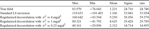
Statistics of the true (simulated) block-mean gravity anomalies Δg, in comparison with the statistics of the estimated block-mean gravity anomalies obtained from: (i) standard LS inversion (Δg^LS) and (ii) regularized decorrelation for varying values of the a priori constrained error variance (all values in mgal).

Open in new tabDownload slide

Alternatively, the inversion of the gradiometric data Tⁱ_rr is performed using the CV-adaptive regularization scheme by constraining the CV matrix of the estimated gravity anomalies to a specific a priori model. In particular, we examine three different constraint choices all of which correspond to a diagonal matrix of the general form . In this way, it is ensured that the parameter estimation errors during the downward continuation process become uncorrelated (i.e. ‘whitening’ of the estimated gravity anomalies) and they have a common user-dependent variance. The value of σ has been set equal to 2, 1 and 0.5 mgal, respectively. The results obtained from this CV-adaptive decorrelating inversion scheme are presented in Tables 2 and 3.

From the error statistics shown in Table 3, we see that there is a clear improvement in the downward continuation results when using the CV-adaptive regularized estimator. By setting the error standard deviation in the estimated gravity anomalies σ = 1 mgal, for example, the rms error drops from 48.53 mgal (standard LS inversion) to 27.75 mgal. There is of course a remaining bias in the estimated gravity anomalies that amounts to about 3.4 mgal on average, which is nevertheless well below the statistical uncertainty of the results. It must be noted that, as the value of the a priori constrained error variance σ² becomes smaller, the corresponding bias in the results of downward continuation decreases considerably (see Table 3). In this way, when we set σ = 0.5 mgal, then the rms estimation error is reduced to 21.67 mgal and the average bias drops to approximately 1 mgal. However, the trade-off in this case lies on the oversmoothing that takes place in the resulting grid of block-mean gravity anomalies, as seen in the values of Table 2.

5 Summary and Conclusions

A new approach for constructing optimal parameter estimators for the inversion of linear models has been presented in this paper. Our methodology is based on a linear transformation of the classic LS estimator and it adheres to two basic criteria. First, it provides a solution that is optimally fitted (in an average quadratic sense) to the classic LS parameter solution. Secondly, it complies with an external constraint that specifies a priori the error CV matrix for the estimated model parameters. The MSEE performance of the new estimator, as well as its optimality with respect to the maximum size of its inherent bias, have been explained and analysed. Furthermore, an expression for the admissible SNR range of the underlying linear model has been derived, within which the new estimator always outperforms (in the MSEE sense) the usual LS solution.

The paper does not claim the development of an autonomous regularization method that competes against other well-known inversion techniques, such as Tikhonov—Philips regularization, GRR or TSVD estimation. The aim of the paper was to present a certain theoretical formulation, based purely on statistical concepts and criteria, for the optimal inversion of linear models that leads to a general CV-adaptive biased estimator. It has been shown that the spectral representation of this parameter estimator offers a unified treatment for existing regularization methods in ill-posed inverse problems, particularly for those techniques that are based on the eigenvalue filtering of the inverse normal matrix. Our study provides an alternative viewpoint on the optimal statistical properties and the regularization mechanism of many inversion techniques commonly used in geodesy, by interpreting them as a family of ‘CV-adaptive’ parameter estimators that obey the same optimal criterion (i.e. optimal fitting with the LS solution in the mean squared sense) and differ only on the pre-selected form of their error CV matrix under a fixed model design.

Further studies and experimentation is obviously needed for the assessment of the practical potential associated with our proposed theoretical methodology in linear model inversion. The results obtained from a simulation experiment that was presented in this study certainly provide some encouragement for exploring new innovative strategies in ill-posed geodetic inverse problems (e.g. regularized decorrelation or optimal ‘whitening’ of the estimated model parameters).

Acknowledgments

The author would like to acknowledge the valuable suggestions and comments on the original manuscript by two anonymous reviewers, which led to an improved revised version of this paper.

References

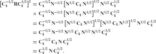
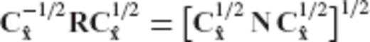
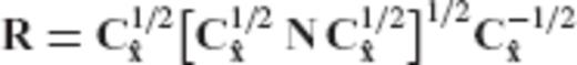
Appendix A: Determination of the Optimal Regularization Matrix

Given the usual LS estimator and its associated CV matrix for an unknown parameter vector x in the linear model , we seek an optimal regularization matrix R such that the biased estimator

(A1)

minimizes the quadratic form

(A2)

and satisfies the following CV-adaptive constraint

(A3)

where is a given symmetric positive-definite matrix. To a large extent, the proof that follows adheres to a similar derivation given in Eldar & Oppenheim (2003).

Let us first apply an auxiliary invertible transformation to the vectors and , as follows

(A4)

(A5)

In this way, the original quadratic form in eq. (A2) can be equivalently written as

(A6)

The CV matrices of the transformed vectors and will be given by the equations

(A7)

(A8)

Following from eq. (A1), the relationship between the transformed estimators and is expressed in terms of the linear equation

(A9)

where the matrix is related to the original regularization matrix R in terms of the transformation formula

(A10)

Let us consider the eigenvalue decomposition of the CV matrix given in eq. (A7)

(A11)

where V is a unitary matrix whose columns correspond to the orthonormalized eigenvectors of , and D is a diagonal matrix that contains the eigenvalues of .

Using the unitary matrix V, an auxiliary invertible transformation will now be applied to the vectors and , as follows

(A12)

(A13)

Due to the orthogonality of the matrix V^T, the quadratic form in eq. (A6) can be equivalently expressed as

(A14)

The CV matrices of both transformed vectors and are now diagonal, since

(A15)

(A16)

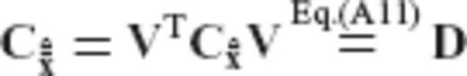
Following from eq. (A9), the relationship between the transformed vectors and is given by the linear formula

(A17)

where the new matrix is related to the previous transformation matrix via the equation

(A18)

Denoting by and the expectation vectors of and , respectively

(A19)

(A20)

the quadratic form in eq. (A14) can be decomposed as follows

(A21)

where the ancillary term ρ corresponds to the quantity

(A22)

Furthermore, we have

(A23)

Taking into account eq. (A16), the quadratic form ϕ from eq. (A21) can be now expressed as

(A24)

where x denotes the true vector of the unknown parameters.

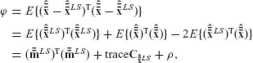
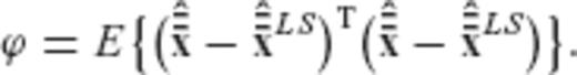
The first two terms in the above equation do not depend on the required regularization matrix R (or on any of its transformed versions and ), and thus the minimization of ϕ is equivalent to the minimization of the third term ρ which was defined in eq. (A22).

Taking into account the linearity of the expectation operator E{·}, we can express the quantity ρ in the alternative form

(A25)

where and denote the kth elements of the vectors and , respectively. Since the auxiliary vector also does not depend on the regularization matrix R (or on any of its transformed versions and ), the minimization of ϕ is thus reduced in finding the elements that minimize the value of ρ as given in eq. (A25).

In order to find the minimum of ρ we will use the well-known cosine inequality (Papoulis 1991, p. 154)

(A26)

which is valid for any pair (x₁, x₂) of real-valued random variables. Note that the equality sign in the previous inequality holds if and only if the random variables are linearly related, , where a is an arbitrary real scalar.

Putting the elements and in place of the arbitrary random variables x₁ and x₂, the cosine inequality of eq. (A26) yields

(A27)

or equivalently

(A28)

By adding the term to both sides of the above inequality, we get

(A29)

and by summing over all possible values of the index k, we finally obtain

(A30a)

or equivalently

(A30b)

The minimum value of ρ is attained when the equality sign in eq. (A30b) holds, and this occurs if and only if the cosine inequality in eq. (A27) becomes an equality for every value of the index k, that is,

(A31)

which obviously holds if and only if the random variables and are linearly related

(A32)

where λ_k denotes an arbitrary scalar factor that depends on the index k.

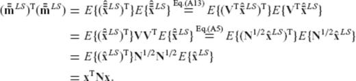
It is important to keep in mind that the elements are uncorrelated with each other with variances equal to one . The elements are also uncorrelated with each other, with variances specified by a given diagonal matrix which depends on the a priori choice of the constrained CV matrix for the original estimated parameters; see eqs (A11), (A15) and (A16). In this way, the proportionality constants λ_k in (A32) can be uniquely specified. Using vector notation, we have that and should be related through a diagonal matrix

(A33)

such that .

Hence, based on the vector transformation formula in eq. (A17), the regularization matrix becomes

(A34)

From eq. (A18), and taking also into account eqs (A7) and (A11), we obtain the regularization matrix

(A35)

Using the last result, the required regularization matrix R is finally determined from eq. (10) as

(A36)

In order to conclude the proof, it is required to show that the above result satisfies the CV-adaptive constraint given in eq. (A3). We have

(A37)

which concludes our proof.

The auxiliary matrices D and Λ which have been used in the previous derivations are not related to the diagonal eigenvalue matrices D and Λ that were introduced in the main body of the paper. In particular, the symbol D in the main paper corresponds to a diagonal matrix containing the eigenvalues of the a priori constrained CV matrix of the estimated parameters ; see (34). The same symbol, however, is also used in Appendix A to denote an auxiliary matrix that plays a supporting role in the presentation of the proof. Similarly, the symbol Λ in the main paper corresponds to a diagonal matrix containing the eigenvalues of the normal matrix N (see (12)), whereas in Appendix A the symbol Λ is employed to denote an auxiliary matrix that plays a supporting role in the presentation of the proof.

Appendix B: An Alternative Formula for the Optimal Regularization Matrix

In Appendix A it was proven that the optimal regularization matrix R in the CV-adaptive estimator is given by the equation

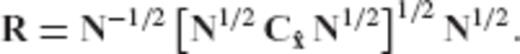
(B1)

Here we shall derive an alternative equivalent expression for the above regularization matrix. From eq. (B1) we have

(B2)

and

(B3)

Taking into account the result of the last formula, we can write that

(B4)

and finally

(B5)

which gives an alternative expression of the regularization matrix in eq. (B1).