


Summary
A grid of 32 across-axis and five axis-parallel multichannel seismic (MCS) reflection profiles were acquired at an axial volcanic ridge (AVR) segment at 57° 45′N, 32° 35′W on the slow-spreading Reykjanes Ridge, Mid-Atlantic Ridge, to determine the along-axis variation and geometry of the axial magmatic system and to investigate the relationship between magma chamber structure, the along-axis continuity and segmentation of melt supply to the crust, the development of faulting and the thickness of oceanic layer 2A.
Seismic reflection profiles acquired at mid-ocean ridges are prone to being swamped by high amplitude seabed scattered noise which can either mask or be mistaken for intracrustal reflection events. In this paper, we present the results of two approaches to this problem which simulate seabed scatter and which can either be used to remove or simply predict events within processed MCS profiles.
The 37 MCS profiles show clear intracrustal seismic events which are related to the structure of oceanic layer 2, to the axial magmatic system and to the faults which dismember each AVR as it ages through its tectono-magmatic life cycle and which form the median valley walls. The layer 2A event can be mapped around the entirety of the survey area between 0.1 and 0.5 s two-way traveltime below the seabed, being thickest at AVR centres, and thinning both off-axis and along-axis towards AVR tips. Both AVR-parallel and ridge-parallel trends are observed, with the pattern of on-axis layer 2A thickness variation preserved beneath relict AVRs which are rafted off-axis largely intact.
Each active AVR is underlain by a mid-crustal melt lens reflection extending almost along its entire length. Similar reflection events are observed beneath the offset basins between adjacent AVRs. These are interpreted as new AVRs at the start of their life cycle, developing centrally within the median valley. The east–west spacings of relict AVRs and offset basins is ∼5–7 km, corresponding to a life span of the order of 0.5–0.7 Myr, during which AVRs appear to undergo multiple 20–60 Kyr tectono-magmatic cycles.
1 Introduction
Numerous sub-seabottom geophysical experiments have been conducted on the mid-ocean ridge system to investigate the dynamics of crustal accretion, the morphology of spreading centres, and the evolution of oceanic crustal structure. Detailed seismic experiments at fast- and intermediate-spreading ridges (examples include: Rohr 1988; Harding 1989, 1993; Detrick 1987, 1993, 1994; Burnett 1989; Collier & Sinha 1990, 1992a, b; Kent 1990, 1994, 2000; Toomey 1990; White & Clowes 1990; Caress 1992; Carbotte 1997; Christeson 1992, 1996; Cudrack & Clowes 1993; Toomey 1994; Vera 1990; Vera & Diebold 1994; Mutter 1995; Hussenoeder 1996, 2002a; Grevemeyer 1997; Hooft 1997; Turner 1999; Dunn 2000; Day 2001; Tong 2002; Blacic 2004; Sohn 2004) have revealed the fine-scale structure of the uppermost crust, and low-velocity zones and reflection events associated with the axial magmatic system. Such studies (e.g. Kent 1993a, b, 2000) have begun to relate structures within the crust to the various scales of morphological and petrological segmentation evident from topographic studies (e.g. Macdonald 1984, 1988) and sampling (e.g. Langmuir 1986; Sinton 1991; Auzende 1996), while others (e.g. Turner 1999; Bazin 2001; Day 2001; Peirce 2001) have begun to reveal the connectivity of adjacent ridge segments via their melt supply. This work has, therefore, begun to provide important constraints on the dimensions, physical state, along-axis continuity and geometry of the crustal melt reservoir and the development of the internal structure, seabed morphology and spreading dynamics of the oceanic crust.
In contrast, numerous seismic studies undertaken at the slow-spreading Mid-Atlantic Ridge (MAR) have shown little, or no evidence, for a significant crustal melt body (cf.Calvert 1995 and Detrick 1990 and both with Navin 1998) but have begun to reveal the detail of the crustal structure (some examples include: Detrick 1997; Barclay 1998; Canales & Detrick 1998; Smallwood & White 1998; Hussenoeder 2002b; Dunn 2005). However, the fierce topography associated with the rift valley and the large-scale normal faulting (e.g. Carbotte & Macdonald 1990; Shaw & Lin 1993; Escartin & Lin 1995; Escartin 1999; Reston 2004) prevalent at slow-spreading ridges result in seismic profiles that are contaminated with significant high amplitude noise—a consequence of scattering from seabed topography both in- and out-of-the-plane of the profile (e.g. Calvert 1997). These steeply dipping, high-amplitude scattered arrivals mask the lower amplitude intracrustal reflection events. A consequence of this imaging problem is that progress towards understanding the detail of intracrustal and uppermost mantle processes at slow-spreading ridges is, in many ways, being made more slowly than for fast- and intermediate-spreading ridge systems, and is dependent on advances in data processing methods to predict and thus remove, or minimize, this scattered energy.
As our ability to image the detail of the seabed topography improves, aided by faster and more powerful computers, it is now becoming possible to undertake such predictions of seabed scatter. In this paper, we present the results of two end-member approaches to this problem and their application to a multichannel reflection data set acquired at the slow-spreading Reykjanes Ridge. By then combining the seismic results with other geophysical data sets we develop an integrated model for axial volcanic ridge formation and evolution, tectono-magmatic cycles, asymmetric ridge spreading and ridge segmentation.
2 Setting
The Reykjanes Ridge, part of the MAR south of Iceland, is a particularly good example of a highly segmented, slow-spreading ridge system (Fig. 1; e.g. Murton & Parson 1993; Parson 1993; Applegate & Shor 1994; Searle 1994; Taylor 1995; Sinha 1997, 1998; Searle 1998; Peirce & Navin 2002; Peirce 2005). The axial seafloor in the study area is dominated by a shallow median valley and the presence of a series of well-defined, en echelon, axial volcanic ridges.
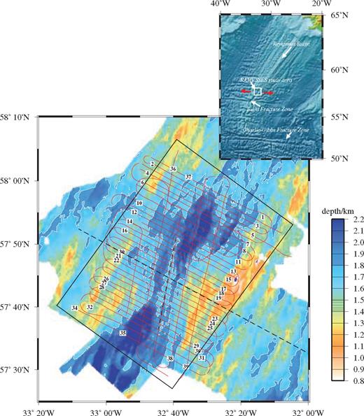
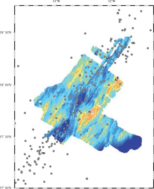
Bathymetric map of the study area on the Reykjanes Ridge, showing the location of all MCS profiles acquired during RAMESSES II. The 1800 m bathymetric contour is shown in white to outline the median valley and each AVR. Red lines show profile locations, with profile numbers marked in black. The black dashed lines show the location of the coincident MCS and wide-angle profiles acquired during RAMESSES I (Navin 1998). The solid black line shows the location of the region shown in Fig. 15. The inset shows the bathymetry of the North Atlantic (from Sandwell & Smith 1997) with the location of the study area outlined by the white box and the red arrows showing the spreading direction. The transition from axial high to median valley morphology can be seen at ∼59°N. The Bight fracture zone marks the end of the Reykjanes Ridge and is located at the change in ridge trend at ∼57°N.
The first RAMESSES project (Reykjanes Axial Melt Experiment: Structural Synthesis from Electromagnetics and Seismics; Sinha 1997, 1998) targeted an axial volcanic ridge (AVR) segment at 57° 45′N. Interpretation of seismic refraction and controlled-source electromagnetic (CSEM) data from the first RAMESSES cruise (henceforth RAMESSES I—RRS Charles Darwin CD81/93 —Sinha . 1994), revealed the presence of a substantial crustal magma chamber beneath this AVR (Navin 1996; Navin 1998; MacGregor 1997; MacGregor 1998). Ray trace modelling of wide-angle refraction data, interpretation of a reversed polarity reflection event in an along-axis fourfold multichannel seismic (MCS) profile and analysis of CSEM data indicated that the magma chamber comprises a thin, sill-like body containing a high proportion of melt, underlain by a larger volume of ‘mush’ consisting primarily of solid crystals, but with up to 20 per cent partial melt distributed through it. These features are consistent with a robust axial magmatic system, similar to that found beneath faster spreading ridges and suggest that, in many respects, similar processes occur during crustal accretion at all spreading rates. The combined interpretation of high-resolution sonar, gravity, magnetic, CSEM and magnetotelluric (MT) data with the seismic model, provided strong evidence that crustal construction is occurring not as a steady-state process, but in cycles of magmatic accretion followed by tectonic extension (Sinha 1997, 1998; Navin 1998; MacGregor 1998; Heinson 2000; Peirce & Navin 2002; Peirce 2005), with the duration of such a cycle—a tectono-magmatic cycle—being of the order of 20 000–60 000 yr.
The objective of the second RAMESSES study (henceforth RAMESSES II—RRS Discovery D235c/98; Peirce & Sinha 1998) was to collect a grid of MCS reflection profiles in order to determine the along-axis variation and geometry of the axial magmatic system and to investigate the relationship between magma chamber structure, the along-axis continuity and segmentation of melt supply to the crust, the development of faulting and the thickness of oceanic layer 2A. In this paper, we present the results of interpreting the grid of MCS profiles acquired during RAMESSES II.
3 Acquisition
Using a 96-channel, 25 m group interval streamer, 32-fold data were recorded while surveying at a speed of 9 km hr−1. The seismic source comprised 12 airguns of varying chamber sizes totalling ∼5175 in3 volume (∼85 l) which were fired at 2000 psi (13.8 M Pa) pressure and with a shot interval of 15 s. Data were recorded at 4 ms sampling over a trace length of 10 s.
A grid of 32 axis-perpendicular and five axis-parallel MCS profiles was acquired (Fig. 1), with across-axis profiles spaced at ∼1.5 km intervals and along axis-profiles at 5 km intervals—the latter representing ∼500 000 yr age intervals at the average half spreading rate of 10 mm yr−1. With this geometry, 3-D structures could be interpolated between 2-D lines. Two of these profiles, intersecting at the centre of the AVR, were coincident with the original RAMESSES I across-axis (grid line 20) and along-axis (grid line 37) refraction and fourfold reflection seismic profiles. These profiles were re-shot in order to tie the new MCS images to the constraints on sub-seafloor structure determined by the previous geophysical studies, as well as to provide well constrained velocity models for seismic processing. A number of the across-axis profiles were located north and south of the ends of the RAMESSES I AVR, to investigate magma chamber continuity between adjacent AVRs. The four axis-parallel profiles were acquired to investigate how crustal structure varies with age. The overall aim was to construct a detailed 3-D crustal reflectivity model of the AVR and neighbouring crust to the north and south, extending up to 20 km (2 Myr) off-axis.
4 Seismic Imaging
The 2-D RAMESSES II profiles contain significant seabed scattered energy, both for profiles acquired parallel and perpendicular to the trend of the most significant scattering surfaces—namely the fault scarps at the edges of the median valley (Fig. 2). Although a 3-D grid of profiles was acquired, with line spacings adequate to enable mapping of reflecting horizons within a 3-D volume, the profiles were not sufficiently closely spaced to allow full 3-D processing. The 2-D data processing undertaken is briefly outlined below, together with a description of approaches that we adopted to minimize the scattered signal.
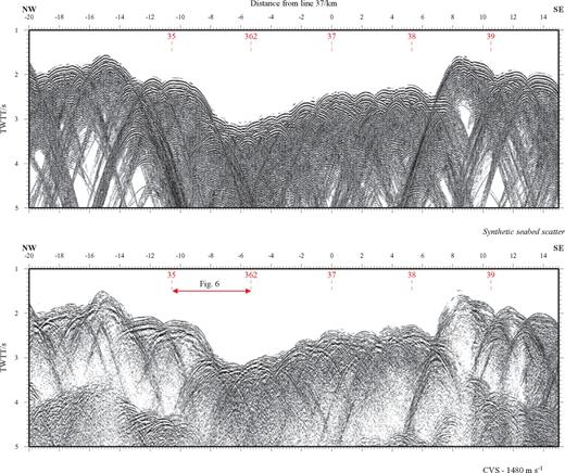
TWTT section of across-axis line 30 (lower panel) stacked at a constant velocity of 1480 m s−1 to show the scattered wavefield associated with the rough seabed. Intersections with axis-parallel profiles are shown by vertical red dashed lines. Much of the intracrustal reflectivity is obscured by the high amplitude scattered wavefield. The upper panel shows corresponding synthetic seismograms calculated using the ‘quick and simple’ approach plotted with matching display parameters. The location of the data enlarged for Fig. 6 is annotated.
4.1 Standard data processing
Numerous equipment problems were experienced throughout acquisition which are summarized in Peirce & Sinha (1998). These led to difficulties in geometry assignment, and required the application of detailed source and receiver statics and corrections for source signal amplitude and dominant frequency variation.
For geometry assignment, all source and receiver locations were determined in x, y, z coordinates (offset in x, y, (m) and depth below sea surface (m)) with 0,0,0 being located at the sea surface at 57° 45′N 32° 41′W—the intersection of the original RAMESSES I across- and along-axis MCS and wide-angle profiles (and consequently the intersection of grid lines 20 and 37 of RAMESSES II). Individual source and receiver depths were used to calculate static corrections which were then applied to correct each shot gather to the sea surface datum.
Following sorting to CMP gathers, pre-stack predictive deconvolution and bandpass filtering (5–50 Hz) were applied to reduce incoherent noise and minimize source signature reverberation. The data were then stacked using a normal move-out (NMO) velocity model derived from a combination of the RAMESSES I wide-angle velocity model, semblance analysis and constant velocity stack (CVS) panels. This combined approach to velocity analysis showed that intracrustal reflection events are best imaged with CVS sections. Although a time variable velocity model was produced for final section generation, migration and depth conversion, most sections shown in this paper are plotted as CVSs, with stacking velocities tailored to highlight specific reflecting horizons. The velocity models are as follows:
Constant 1480 m s−1– to image the seabed.
Constant 1700 m s−1– to image the layer 2A/2B transition.
Constant 2100 m s−1– to image any melt lens events similar to those imaged in the along-axis RAMESSES I profile (Navin 1998).
Variable – to image the entire upper crust.
Extensive data processing tests showed that the simplest approach tended to give the best results. The same processing scheme was, therefore, applied to each of the 37 profiles, comprising: amplitude recovery, shot-receiver statics, trace edit, sorting, pre-stack deconvolution and bandpass filtering, normal move-out correction and stacking. The velocities were chosen from the above, to best highlight specific intracrustal events or to provide an overall image of the entire section. In some cases this was followed by migration.
Although this simple, standard approach to data processing was found to give the best results for the majority of profiles, it had a limited effect on the seabed scattered signal. Frequency-wave number (FK) dip move-out (DMO) and FK migration (pre- and post-stack) were also tested as a means of reducing this signal (Kent 1996), and as a means of correctly positioning the seafloor and minimizing the distortion resulting from NMO-based constant velocity stacking as described below.
4.2 Dipping reflecting horizons
The standard approach to MCS data processing is founded on the assumption of planar and horizontal reflectors. In many cases this assumption is also valid where reflector dip is shallow and occurs over a distance longer than the acquisition foot print at each reflecting horizon.
However, at mid-ocean ridges this basic assumption clearly breaks down. The common depth reflecting point is significantly laterally smeared and the sections are distorted both laterally and vertically. In cases of significant reflector variability, full 3-D acquisition and processing should ideally be applied, with processing based upon algorithms designed to accommodate steep dips. Such a fully 3-D data set was acquired by Kent (2000) at the EPR, where the seabed is significantly smoother due to the faster spreading rate. However, even application of fully 3-D processing to that data set was unable to fully suppress or correctly migrate the entire seabed-scattered wavefield. For the 2-D RAMESSES II MCS data, both FK DMO and FK migration were applied to minimize the effect of dip and seabed scattering. Although these processes provided some improvement in section clarity for the along-axis profile, the improvement proved minimal for the across-axis profiles with, in general, much of the seabed scattered energy merely being smeared. This is largely because these methods of 2-D processing are unable to deal with out-of-plane scattered energy. Examples of the results of the standard and dipping approaches to processing are shown throughout this paper.
4.3 Simulating seafloor scattering
As Fig. 2 shows, all of the profiles are dominated by noise associated with scattering of the down-going wavefield by the rough median valley and AVR seabed topography. It is often argued that intracrustal events seen on MCS profiles at mid-ocean ridge axes may merely be scattered events. It is, therefore, vital to suppress this scatter, or at the very least be able to distinguish it from any real events that it may obscure, before any form of interpretation can take place.
Two end-member approaches were adopted. The first aims to synthetically recreate the seafloor-scattered signal, so that it can be compared directly with the real data, and the identified scatter events preferentially muted (suppressed) during the early stages of processing prior to stacking. The second aims solely to synthetically recreate the scatter signal for direct comparison with observed stacked data sections only.
The former modelling of the seabed in three dimensions requires a full wavefield approach. To enable direct comparison of synthetic model results with observed data also requires replication of the pre-stack (i.e. multireceiver) amplitudes as well as traveltimes. The latter approach can be far more simplistic since its goal is only to identify events most likely to be of a scattered origin such that they can be ignored during interpretation. Both end-member approaches to the scatter simulation require the seabed topography to be known with a resolution better than the Fresnel zone width at the seabed corresponding to the seismic data characteristics. The highest resolution swath bathymetry data available have been compiled by Keeton (1997) and this was used for all modelling.
4.3.1 Phase screen modelling
Computing pre-stack synthetic data from a 3-D representation of the seafloor for each of the 37 profiles using a standard finite difference approach would be prohibitively computationally expensive, taking perhaps several years to compute a synthetic version of just one of the profiles being analysed. The phase screen method (Wild & Hudson 1998; Wild 2000; Hobbs 2003) provides an alternative which is considerably faster, although it does have certain inherent limitations.
Wild & Hudson (1998) summarize the approach as amounting ‘to a reduction of the heterogeneous model medium…… ..to a sequence of diffracting screens, orientated perpendicular to the predominant direction of wave propagation’. During propagation between screens, the parameters of the medium are assumed to be constant for any wave entering from the same point on the screen, with the values set to that at the entry point. Therefore, the phase screen code is particularly appropriate for computing the response of the seafloor since the model comprises a uniform medium (the water column) with a single interface (the seabed).
To replicate the seabed scattering in this study, only P-waves were considered. One of the advantages of this method is that the individual screens need not be equally spaced. The screen spacing in the water column can be much greater than that in the region of the seafloor so that computation time is not spent unnecessarily calculating the seismic response of sea water. An example of the parametrization approach is shown in Fig. 3.
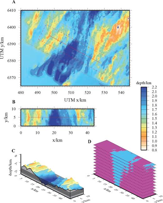
Illustration of the parameterization used for the phase screen modelling. (a) Extract from the swath bathymetry compilation of Keeton (1997) showing the profile (red solid line) to be modelled. The red dotted line shows the area of seabed included in the modelling. (b) Rotated bathymetry grid to be input to the model (red dashed area from a). (c) 3-D representation of the input model, showing the seabed (bold black solid line) and the location of the horizontal screens (thin solid lines). (d) The velocity and density are defined on a regular grid of nodes on each screen where, in this example, the water column P-wave velocity (blue) is 1480 m s−1, while the sub-seabed P-wave velocity (pink) is 3000 m s−1.
Before commencing with parametrization, the resolution of the swath bathymetry data must be considered in the context of the Fresnel zone width at the seabed. Keeton 's (1997) bathymetric compilation has a horizontal resolution of 200 × 200 m. For the average water column velocity, dominant source frequency band and average depth to the seabed, the diameter of the Fresnel zone is approximately 200 m for reflections from a horizontal seafloor. However, sidescan sonar images show that significant variation in seabed topography occurs vertically and laterally on wavelengths shorter than this. The effect this has on the calculation of the scattering is that, although the small-scale features lead to short wavelength variations in the amplitude of the primary arrivals, they do not significantly affect the traveltimes nor do they generate the larger-scale scattering events identified throughout the data sections. Therefore, Keeton 's (1997) swath bathymetry data compilation was considered sufficiently accurate to undertake the scatter forward modelling using the phase screen method.
The objective of the phase screen modelling is to predict and identify scatter to a two-way traveltime (TWTT) just above the first sea surface multiple, thus minimizing computation time (since the multiple largely obscures all other coherent reflection events). Ideally, it should be possible to subtract the synthetic events from the real data. However, this would require exact phase and amplitude matching and the application of accurate statics to the real pre-stack data to ensure a consistent datum. An alternative approach is to pick the TWTT of arrivals common to both the real and synthetic gathers at the pre-stack stage, and construct surgical mutes to remove the scattered energy from the real data. The cleaned gathers are then processed as outlined above. It is important to note that both in- and out-of-plane scattered arrivals are simulated and (in principle) suppressed by this approach.
The first stage of muting the seafloor scattered energy is to compute synthetic shot gathers for an entire MCS line. The main requirements (Fig. 3) are a velocity model; the seafloor topography along the profile and out-of-the-plane to two streamer lengths (5 km) either side; the acquisition geometry; and the frequency content of the seismic source. Each synthetic gather takes ∼1 hr of CPU time on a six-processor machine to compute and, hence, an entire profile of gathers takes ∼6 weeks. However, although the synthetic gather spacing needs to be small so that arrivals from common features can be tracked between them, the horizontal resolution of the swath bathymetry data defining the model seafloor is only 200 × 200 m. Therefore, as it is expected that shots with a smaller spacing than 200 m would show little variation, the synthetic shot spacing was set at 112.5 m, the equivalent of modelling every third shot, which reduced computation time significantly.
Having calculated the synthetic gathers, these are compared with the real data gathers on a shot-by-shot basis (Fig. 4) and common arrivals are picked. A ramped trapezium surgical mute is then defined and applied on a trace-by-trace basis at the gather level for each common arrival (Fig. 5). A similar muting process, this time done on a channel-by-channel basis between gathers, is also applied to the seabed primary reflection, since the TWTT of this event is perturbed significantly on the far-offset channels by the rough seafloor. The data are then processed to stacked section as described above. Fig. 5 shows example scattered arrival picks and the mute definition.
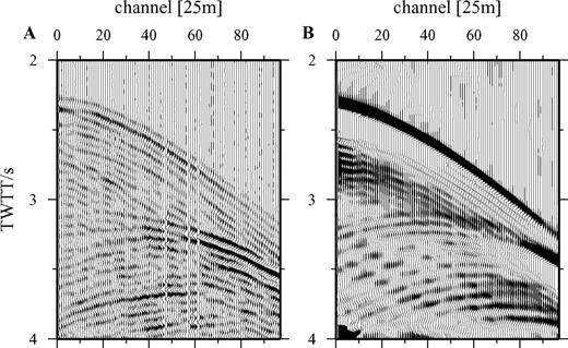
Examples of real (a) and corresponding synthetic (phase screen) (b) shot gathers. In (b) only the primary seabed reflection and the seafloor scattered signal have been modelled. For this example, almost all of the signal in (a) is scatter. Direct comparison of shot gathers allows scattered parts of the wavefield to be distinguished from sub-seabed reflections.
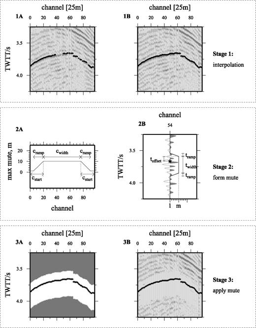
Scatter muting process applied to a single shot gather from line 30. Stage 1: TWTT picks (black stars in 1a) defining each identified scattered event are interpolated between traces within the shot gather (1b), and then interpolated for each common channel between shot gathers. Stage 2: The shape (2a) and position (2b) of the mute window are defined around each of the picks. Stage 3: The mute window defined in stage 2 (3a) is applied to the gather (3b) to suppress the scattered signal.
To illustrate the effectiveness of the muting process, Fig. 6 shows a comparison of constant velocity stacks made using pre-stack muted data and the equivalent un-muted data. In this figure it can be seen that the muting has removed much of the scattered energy. Since this removal takes place before stacking, weaker arrivals that were otherwise masked by high amplitude scattered noise are now visible. This figure also shows how relatively ineffective 2-D DMO and migration processing are for the across-axis profiles.
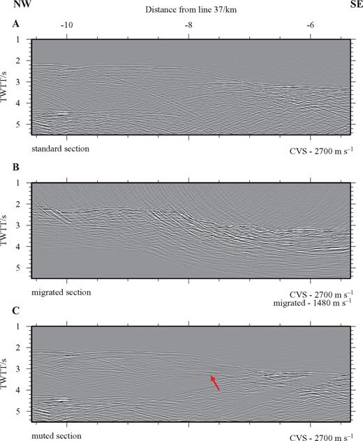
Results of the phase screen muting process for line 30. (a) Un-muted CVS section between crossing along-axis lines 35 and 362 (see Fig. 2). (b) Un-muted CVS section shown in (a), migrated to show that standard processing does little to mitigate the scattering. (c) CVS section after pre-stack muting of scattered energy. Muting has removed the majority of the scattered energy and revealed an apparent intracrustal arrival (highlighted by the arrow) that is not visible in either (a) or (b).
Although this procedure is very effective, each minimized set of synthetic gathers that comprise a synthetic profile still takes many days of CPU time followed by days of manual picking prior to the muting stage. An alternative, opposite end-member approximation approach was, therefore, developed as a complimentary analysis tool, and is outlined in the next section.
4.3.2 ‘Quick and simple’ method
An alternative strategy for dealing with the seafloor scattering problem is to adopt an approach that is purely predictive at the final stacked section level, and which uses the synthetic results purely as an identification tool rather than a means by which to remove or subdue unwanted arrivals. Ground-truthing against the phase screen results has allowed us to apply this approach widely and with confidence throughout the data set. Another advantage is that the ‘quick and simple’ method can predict diffraction tails to longer TWTTs than can readily be calculated by the phase screen approach.
The method is outlined below. It is based on a simplification to Kirchoff-Helmholz theory (e.g. Hilterman 1970; Trorey 1970) and assumes coincident sources and receivers to simulate stacked MCS sections as outlined in, for example, Cao & Kennett (1989).
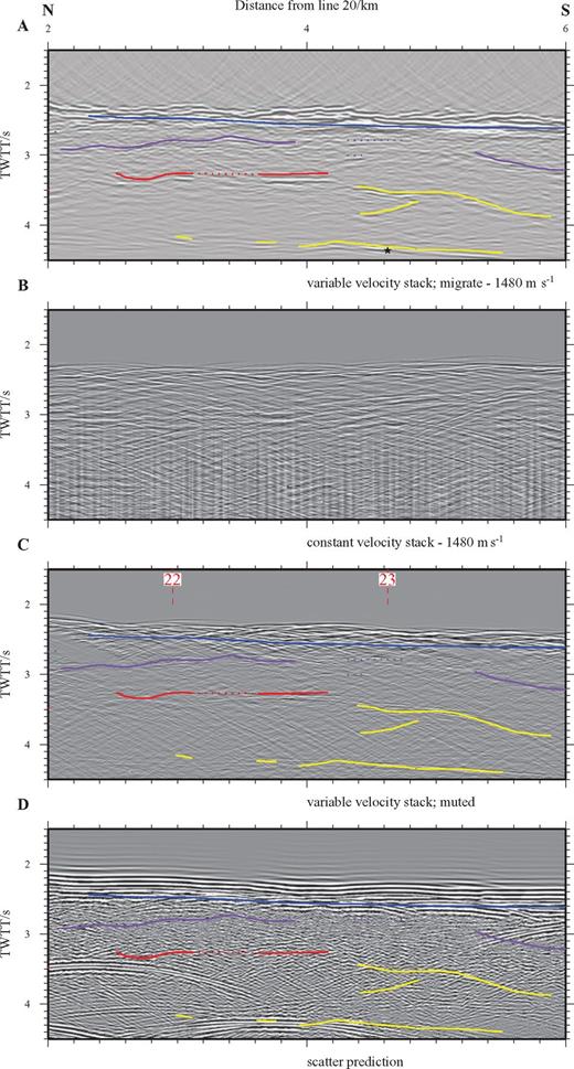
Initially, the entire bathymetry data set is gridded at a node interval matching the common mid-point (CMP) spacing, whilst avoiding spatial aliasing—in this case 25 m. For each CMP position along a profile, a region 2.5 times the streamer length in all directions (6700 m) is selected. The traveltime to each bathymetric cell (assuming coincident source and receiver) within this 144 km2 region is calculated assuming direct water waves and a constant sea water velocity (1480 m s−1). The azimuth, angle of incidence at, and reflection coefficient across the seabed are also calculated and any ray paths incident at greater than 45° rejected. All traveltime estimates are then used to synthetically create an effective reflectivity function by applying a spherical divergence correction to the signal amplitudes and summing the contributions in 4 ms (the sampling interval) time bins progressively beneath each CMP position. As this method approximates data acquisition with coincident source and receiver, it generates a simple CMP stack representation where the stacking velocity is effectively 1480 m s−1. An example of the effective reflectivity is shown, and can be compared directly with the corresponding real CVS data, in Fig. 2. This approach takes only ∼20 s of CPU time per CMP on a single processor machine and, although ‘quick and simple’, does allow direct comparison with the real data to the extent of being able to identify the events most likely to have a scattered origin in the stacked sections. Fig. 2 shows synthetic seismograms calculated using this approach by convolving the effective reflectivity with a representative wavelet.
4.4 Approach to interpretation
Initially, each profile was scrutinized to identify events most likely originating from scatter at the seabed using the ‘quick and simple’ approach. This was then ground-truthed against the phase screen results especially at shallow, sub-seabed depths where the scattering is most significant. For grid line 20 (across-axis) and grid line 37 (along-axis), a direct comparison was also made between events determined by this process to be of intracrustal origin and those predicted from the wide-angle models of Navin (1998) (e.g. the oceanic layer 2A/B and 2/3 boundaries and the Moho) or imaged within the RAMESSES I MCS data (e.g. Figs 7–10). This enabled us to determine the most likely origin of each set of reflection events. It also allowed us to determine specific characteristics which could then be used to identify the various reflectors, and applied to all profiles propagating out from the intersection points of grid lines 20 and 37. Further forward modelling, including sub-seafloor velocity structures, of pre-stack gathers was then undertaken (e.g. Figs 11 and 12) to confirm (or otherwise) the interpretation of each event, and as a means of ensuring interpretation consistency throughout all profiles.
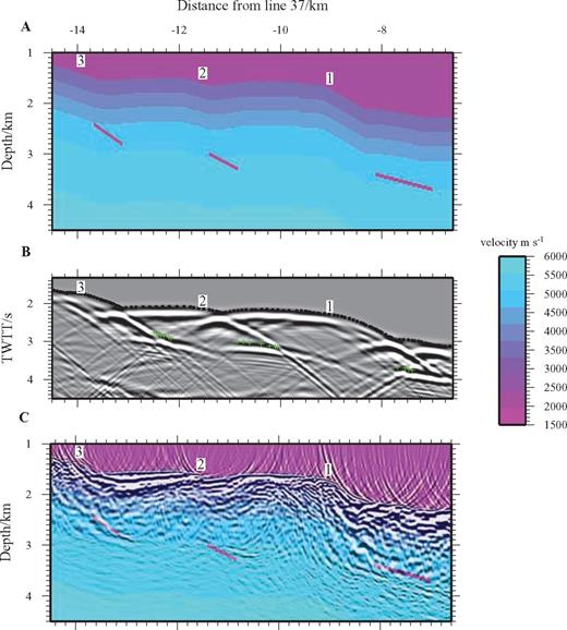
Final TWTT sections for line 30—across-axis. (a) Stack with variable velocity model NMO and low-pass filtering applied. Compare with Fig. 2 for a CVS version of this profile. Intersection points with other axis-parallel profiles are shown by the red vertical dashed lines. (b) Interpretation derived from all TWTT-based versions of this profile. The grey dash-dot lines show the TWTT to the seabed, layer 2A/2B and layer 2/3 boundary, as interpreted from analysis of the RAMESSES wide-angle data by Navin (1998). The TWTT to these horizons was calculated using a 1-D version of the along-axis wide-angle model hung beneath the seabed reflection in the MCS data. The reflection events in the MCS data set have been colour-coded (blue, red and green) according to their identification – see text for details. The lower dotted black line shows the location of the seabed-sea surface multiple.
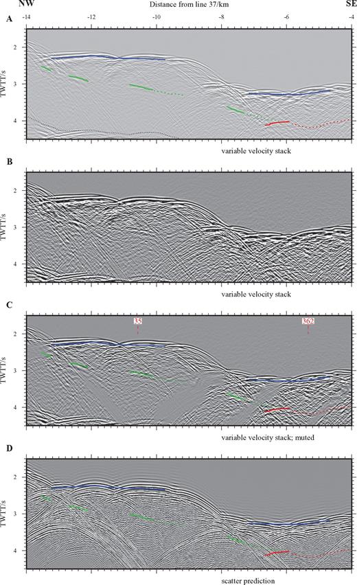
Enlarged view of a section of line 30—across-axis. (a) Interpretation showing event picks. (b) Variable velocity stack TWTT section for comparison. Phase screen muted section (c) and ‘quick and simple’ scatter prediction (d) annotated with event picks. Note that none of the picked events correspond to seabed scatter and that they have been significantly enhanced by the muting process. Compare with Fig. 7 which also contains an outline of display parameters.


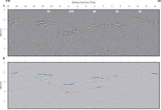
Final TWTT sections for line 37—along-axis. (a) Interpretation derived from all TWTT-based versions of this profile. The reflection events in the current MCS data set have been colour-coded (blue, red, purple and yellow) according to their identification—see text for details. The stars and diamonds show TWTTs to high amplitude scattered arrivals identified on the synthetics for the intersecting across-axis MCS lines. The stars indicate energy originating from a point to the east of this MCS line, while the diamonds indicate energy originating from the west. There is a good agreement between the TWTT of this scattered energy and the arrival highlighted in yellow. This section has been constant-velocity migrated at 1480 m s−1. (b) 1480 m s−1 CVS unmigrated section showing the full extent of the seabed scatter for direct comparison. (c) Variable velocity, pre-stack FK DMO, muted using the phase screen approach to remove seabed scattered signal. Intersection points with across-axis profiles are shown by the red vertical dashed lines. All horizons interpreted as real intracrustal events in (a) are also present in this section. However, the maximum modelled traveltime of the phase screen synthetics is shallower than the yellow event of (a), which is interpreted to be seafloor scattered energy. (d) Scattered wavefield predicted by the ‘quick and simple’ approach. This section corresponds to a 1480 m s−1 CVS, so scattered events are not directly comparable to the yellow events on the migrated section (a).
Enlarged view of a section of line 37—along-axis. (a) Interpretation showing event picks. (b) 1480 m s−1 CVS section for comparison. Phase screen muted section (c) and ‘quick and simple’ scatter prediction (d) annotated with event picks. Note that the picked events have been significantly enhanced by the muting process. Compare with Fig. 9 which also contains an outline of display parameters.
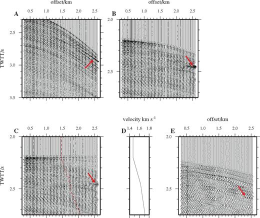
AVO characteristics of the shallow crustal (layer 2A) event. (a–c) CDP super-gathers for line 35 (axis-parallel on 10 Myr old crust outside the median valley). (a) shows the super-gather without NMO correction, while in (b) a constant stacking velocity of 1700 m s−1 has been applied to align horizontally the shallow crustal arrival indicated by the arrow. In (c) a variable stacking velocity has been applied, selected to image the seabed, the shallow crust arrival and any deeper events. The variable NMO velocity function is shown in (d). The shallow crustal arrival in (c) is weaker than in (b) due to the greater NMO stretch associated with the variable velocity stacking. The dashed line in (c) shows the mute that would normally be applied in order to remove any sampled points that had been stretched by more than 30 per cent. (e) Shallow crustal event imaged within a CDP super-gather from line 37 (along-axis profile on zero-age crust). This has been NMO corrected with a velocity of 1700 m s−1. This event has the same AVO characteristics as that shown in (a–c), which suggests it is generated from a horizon whose characteristics do not change significantly with age.
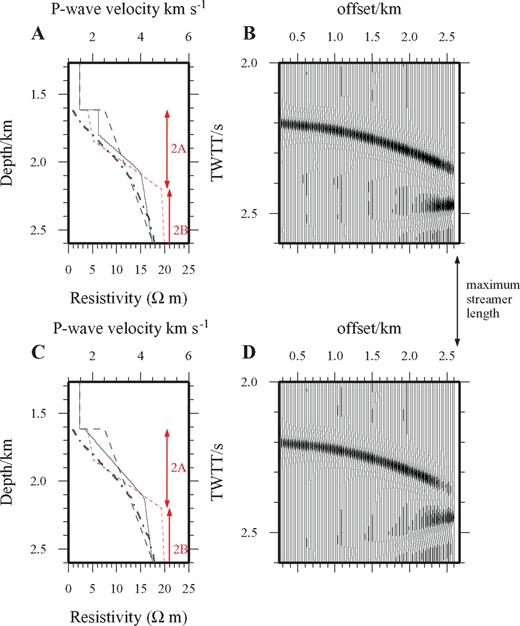
Modelling of the shallow crustal layer 2A (blue) arrival using the 1-D crfl reflectivity code. (a) and (c) show two P-wave velocity models, where the solid black line represents the crflP-wave velocity model, the blue dashed line shows the on-axis wide-angle P-wave velocity model of Navin (1998), while the red dashed lines and red labels show the P-wave velocity model from the EPR of Harding (1993). Also shown in both (a) and (c) is the CSEM resistivity model (black dash dot line) for the northern end of the RAMESSES AVR (MacGregor 1998). (b) and (d) show crfl synthetic gathers computed using the velocity models shown in (a) and (c) respectively. The gathers have been NMO corrected using a stacking velocity of 1700 m s−1. Both compare favourably with the real data shown in Fig. 11. The preferred model (a) is in good agreement with the results of Harding (1993) and also fits the sub-seabed velocity derived from the wide-angle velocity model of Navin (1998)—confirming that the shallow crustal event (blue) is equivalent to the seismic layer 2A event imaged in many other similar surveys. See text for details. Note that the maximum source-receiver offset for this survey is ∼2.6 km, and that the layer 2A event appears on the far-offset traces only.
Having identified the most likely origin of each observed intracrustal event, every profile was then interpreted using a combination of sections processed with both standard and dipping approaches and using variable and constant velocity models for move-out correction, migration and depth conversion, tailored to suit particular target horizons. Our definition of the various classes of events, their characteristics and examples of their interpretation on sections are described in the next section.
5 Reflection Events and Their Origins
Having identified or suppressed as much of the seabed scattered noise as possible, the 37 final processed sections were interpreted as described above and in the context of their geological setting. The interpretation focuses on five main types of intracrustal events as outlined below. An across-axis profile (grid line 30; Fig. 7) and an along-axis profile (grid line 37; Fig. 9) have been selected to show the main features which are identifiable throughout the data set. Grid line 37 is coincident with the RAMESSES wide-angle model of Navin (1998), and this provides a good velocity control with which to depth convert event TWTT picks. In Figs 7 and 9 identifiable events have been grouped and colour-coded to reflect their interpretation. Events with the same colour code are interpreted to be arrivals from the same, or closely related, horizons. In all cases these can be mapped on adjacent and intersecting profiles, giving confidence that they are real events.
5.1 Shallow crustal event—base of layer 2A (blue)
This event is imaged throughout the majority of the survey area at ∼0.3 s TWTT below the seabed. Inspection of CMP gathers (Fig. 11) shows that this arrival is only imaged on the far offset traces, where the source-receiver offset is greater than 2.1 km. Its presence on only these traces indicates that this event is not a simple reflection from a sharp intracrustal interface. However, the maximum source–receiver offset for this survey is ∼2.6 km and, hence, this event is well sampled on multiple traces.
To ascertain its origin, 1-D forward modelling was carried out using the crfl reflectivity code (Fuchs & Müller 1971). Two best-fitting final models are shown in Figs 12(a) and (c), along with the Navin (1998) on-axis wide-angle velocity model for the RAMESSES AVR and the Harding (1993) on-axis velocity model for the EPR for reference. The main difference between these two models is the fine structure of layer 2A, which in one is a single layer of constant velocity gradient, while in the other is divided into two layers of differing velocity gradient. Comparison of the calculated synthetic gathers (Figs 12b and d) with the real gathers (Fig. 11) shows that the latter provides the better amplitude fit, when considering the relative amplitude between the seabed reflection and the ‘far-offset’ event. Comparing this with the interpretation of Harding (1993) suggests that the shallow crustal event imaged in the RAMESSES data is from the base of layer 2A. We refer to this arrival as an event rather than a reflection since its most likely origin, which the modelling supports, is energy that has turned or partially turned in a steep velocity gradient prior to reflection. Of the two models presented here the model shown in Fig. 12(a) is favoured. This model is more detailed than the upper crustal section of the wide-angle model of Navin (1998), which is to be expected as, in the latter, any upper crustal arrivals are largely obscured at near offset by the large amplitude direct water wave.
When a variable stacking velocity function is used for NMO with an event of this type, the far offset traces are badly affected by NMO stretch and are, therefore, muted during normal processing. Given the AVO characteristics of the layer 2A event, such processing results in it being completely suppressed. As a result it is best imaged within CVS sections, in which neither severe NMO stretch nor consequent muting occur. As the layer 2A event is only evident on the longer offset traces, only traces with source-receiver offsets of 0–500 m (to show the seabed) and 2000–3000 m (to show the layer 2A event) were included during CVS processing to create the sections which were then used to map this event across the survey area. Three examples of the layer 2A event on such sections are shown in Fig. 13.
Layer 2A event. (a–c) Intersecting profiles showing characteristics and continuity of the layer 2A event both axis parallel and perpendicular. The solid black line shows the TWTT to the seabed derived from the swath bathymetry data of Keeton (1997). Profile intersections are indicated by the vertical red dashed lines. The layer 2A event, highlighted by red arrows, can be traced as a coherent event on multiple intersecting profiles. (d) Normal fault cutting the layer 2A event (blue highlighting). The profile has been FK migrated at water column velocity (1480 m s−1) and a seabed mute applied. This shows that faulting post-dates layer 2A creation. The approximate location of the fault is indicated by the green dashed line. The event indicated by the red arrow is a migration artefact and does not relate to any geological feature.
The layer 2A event is prevalent throughout the study area. Its amplitude varies significantly, and this is attributed to seafloor scattering effects. Off-axis it appears at between 0.1 and 0.5 s TWTT below the seabed. On-axis this interval increases to a maximum beneath the shallowest AVR topography, suggesting that layer 2A is thickest at this location (Fig. 14). The along-axis thickness variation of this layer at zero age persists off-axis. The layer 2A event is also observed to be offset by inward-facing normal faults (Fig. 13d).
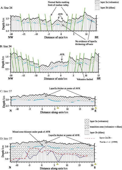
Upper crustal structure at the RAMESSES AVR. (a and b) Interpretations of across-axis lines 24 and 34. The solid blue lines show the depth converted location of the layer 2A events. Between these locations the structure has been interpolated (dashed line). The green lines show the locations of major seabed-offsetting fault planes, which also correspond to offsets of layer 2A. The layer 2A thickness varies along flow-lines as it spreads off-axis (cf.Fig. 15). The pattern of faulting is asymmetric about the ridge-axis. (c) Layer 2A structure along the AVR axis. Layer 2A is thickest below the shallowest bathymetric point of the AVR. The structure below layer 2A, shaded grey, is discussed in the text and is shown in (d). The yellow filled triangles show where lines 24 (a) and 34 (b) cross this profile. (d) Interpreted upper crustal structure along the ridge axis. The solid blue and purple lines show the depth converted location of the layer 2A and purple reflection events respectively. Between these locations the structure has been interpolated (dashed line). The on-axis upper crustal structure is composed of three layers. The thickness of ‘layer 2a (volcanics)’ corresponds with that seen on (a) to (c) and other across-axis lines. The layer marked ‘transition zone (volcanics + dykes)’ was introduced to explain the purple reflector (see Fig. 10). The transition zone has zero thickness directly below the point where the layer 2A is seen to be thickest. The dashed red line shows the depth to the layer 2A/2B boundary of Navin 's (1998) wide-angle velocity-depth model. This does not match the base of layer 2A as interpreted from the MCS data, but shows some agreement with the deeper (purple) horizon.
The velocity function derived from the 1-D modelling was used to convert TWTT picks of this event into depth, although with caution since this event is not a true reflection. Under this assumption any variation in TWTT reflects a change in layer 2A thickness. Fig. 14 shows the inferred depth to the layer 2A/2B boundary along three profiles—two running across-axis (grid lines 24 and 34) and one along-axis (grid line 37). The depth to the base of layer 2A below the seabed is seen to vary between ∼130 and 200 m. On grid line 37, layer 2A is thickest beneath the AVR's shallowest bathymetric point, and thins both north and south towards AVR tips.
In previous studies, the layer2A/2B transition has been variously imaged using a variety of seismic methods and offsets (Harding 1989; Vera 1990; Vera & Diebold 1994; Minshull 1991; Christeson 1992, 1996; Detrick 1993; Harding 1993; Kent 1994; Kappus 1995; Carbotte 1997; Hooft 1997; Kent 2000). The RAMESSES 1 CSEM modelling results (MacGregor 1998; and see Fig. 12) show that the seismic layer 2A/2B transition corresponds with a rapid decrease in porosity. The similarity of the RAMESESS results with those from the EPR and from the drilled section of layer 2 in ODP Hole 504b (Collins 1998) and the Hess Deep (Francheteau 1992), all of which equate the layer 2A event with the base of the extrusive igneous section, suggest that the observations from the RAMESSES area have a similar origin.
Smallwood & White (1998) analysed MCS data further north on the Reykjanes Ridge between 61° and 62°N. They too interpreted the layer 2A event as the base of the extrusive layer and found that its average thickness is 400 ± 100 m. Using the assumption that the extrusive layer corresponds to the magnetic source layer, they were able to model the sea surface magnetic field. Peirce (2005) and Gardiner (2003) show that in the RAMESSES area, the magnetic anomaly and magnetization intensity variation correlate with inferred sites of recent magmatic influx to the crustal magmatic system, and hence regions of likely recent extrusion. Their magnetic intensity solution (Fig. 15) shows that although the longer wavelength trend follows the ridge trend, the shorter wavelength anomalies are associated with AVRs that represent regions of apparently thicker layer 2A. All of these observations support the hypothesis that the layer 2A event represents the base of the extrusive layer, and that this also correlates with the base of the strongly magnetized layer.
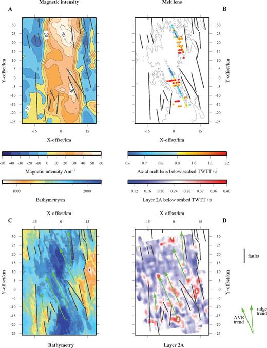
Seafloor magnetization and layer 2A isochron thickness map. (a) Magnetic intensity anomaly showing the central anomaly magnetic high following the ridge trend and the shorter wavelength highs associated with individual AVRs. (b) Melt lens reflector ‘depth’ (in TWTT) below seabed. The 1800 m bathymetric contour is highlighted in grey to show AVR location. (c) Seabed bathymetry for comparison. (d) Layer 2A isochron thickness map showing two main trends in features—AVR-parallel and ridge-parallel. In all parts, major seabed offsets associated with faulting are shown by solid black lines. Layer 2A is thickest and the melt lens deepest near the centre of each AVR.
Fig. 15 shows both AVR- and ridge-parallel trends in the thickness of layer 2A. The ridge-parallel trend is more pronounced outside the median valley, while the AVR-trend is more pronounced within. The vertical displacement of the layer 2A event across faults (Fig. 13) indicates that this layer pre-dates the faulting and originated on or close to the axis. The variation in layer 2A thickness also mirrors the location of relict AVRs observed in the bathymetry data. Extinct AVRs show up both as topographic highs in the bathymetry, and as sites of thickened layer 2A (red shades in Fig. 15d). These features are being rafted off-axis, and displaced vertically by normal faults as, overtime, they are carried up the median valley walls.
5.2 Upper crustal reflector beneath the AVR (purple)
The profile along the AVR axis (grid line 37; Fig. 9) shows an upper crustal event (purple) beneath layer 2A that is not observed on any of the across-axis profiles. The absence of this arrival on the across-axis lines is most likely attributable to imaging problems caused by the steeply dipping topography, which causes de-focusing of energy emerging from the crust. The purple event is not imaged on any other axis-parallel profile or indeed anywhere off-axis, suggesting that it is related to a feature of the very young oceanic crust. The lack of scattered arrivals on the crossing profiles or predicted by the phase screen modelling confirms that this event has an on-axis intracrustal origin.
To investigate this feature, its depth below seabed was calculated from traveltime picks. The velocity model shown in Fig. 12 was used as a starting point. The velocity at the purple event was taken to be 4.5 km s−1 on this basis, in conjunction with Navin 's (1998) wide-angle velocity model.
In DSDP/ODP Hole 504B, the sheeted dyke complex is separated from the extrusive volcanic layer by a transition zone ∼200 m thick and composed of both volcanics and sheeted dykes (Collins 1998). Similarly at the Hess Deep, a transition zone ranging from 50 to 200 m in thickness has been observed in four locations (Francheteau 1992). A change in porosity is reported at the base of the transition zone at Hole 504B. It is feasible that the purple event corresponds to this change in porosity at the base of a transition zone between predominantly extrusive volcanics and predominately intrusive dyke morphologies beneath the AVR (cf.Hooft 1996; Becker 1989; Wilcock 1992). This would be consistent with the results of Greer (2002), who showed that axial crustal porosity at the RAMESSES site decreases from ∼25 per cent in layer 2A to only ∼7 per cent at 1 km depth; and that porosity at the same depth decreases significantly off-axis, which is most likely the result of hydrothermal sealing, over time, of a portion of the porosity (e.g. Anderson 1982). This might explain the absence of a sharp reflecting boundary at this depth away from the axis.
Fig. 14(d) shows the axial upper crustal structure for grid line 37 based on this interpretation. The structure is composed of three layers. The base of the ‘layer 2a (volcanics)’ unit corresponds to the blue event observed on all profiles. The base of the layer marked ‘transition zone (volcanic and dykes)’ corresponds to the purple event observed only on the along-axis profile. Note that the purple horizon is coincident in depth with the base of layer 2A beneath the shallowest AVR topography, where layer 2A is seen to be thickest.
5.3 Mid-crustal reflectors beneath the median valley—axial magmatic system (red)
In Fig. 16 a group of mid-crustal reflectors can be seen beneath the ridge axis (cf.Fig. 9). Comparison with Navin 's (1998) wide-angle seismic velocity model indicates that these features correspond to the top of the axial melt lens. Fig. 15(b) shows the TWTT picks of these events. In common with the base of layer 2A, they are generally deepest beneath the regions of shallowest AVR topography.
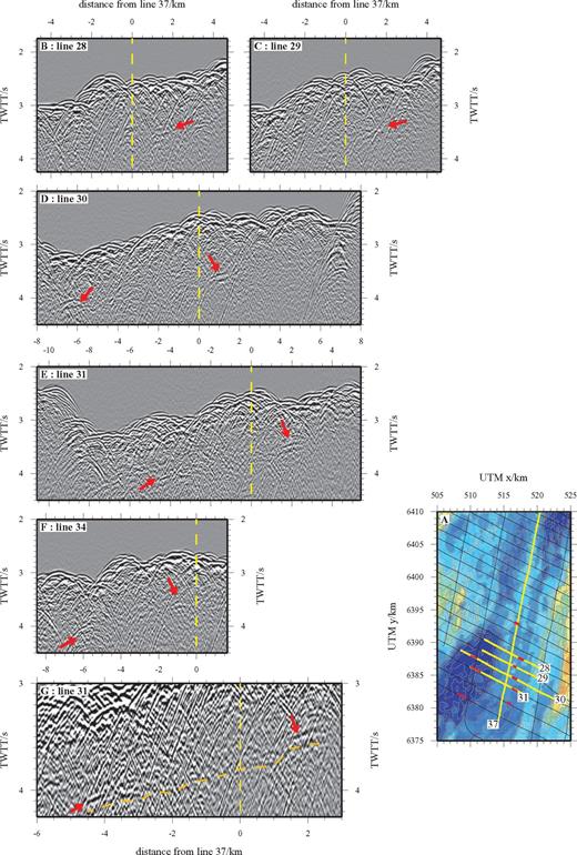
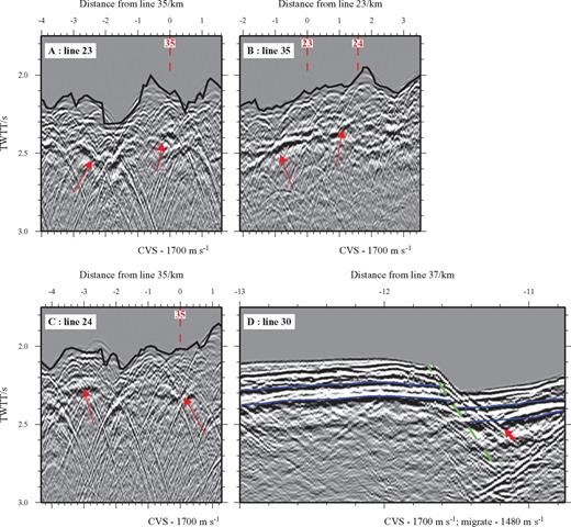
Location of mid-crustal magma body reflections beneath the AVR and southern offset basin. (a) Swath bathymetry basemap contoured at 50 m intervals, marked with the positions of the five seismic sections shown in (b–f) plus the along-axis line 37 (yellow). The thin black lines show the location other profiles that traverse this area. Solid red lines show the locations of all melt lens reflections observed on across-axis profiles from this region. (b–f) show extracts from the final stacked sections for the five profiles plotted as a function of distance from line 37. On each of these sections the reflection event of interest has been highlighted by an arrow. The AVR-axis lies at 0 km offset in all cases. In sections (d) and (e) a weak event links the melt lens events suggesting that the melt supply along-axis may be interlinked. An enlargement of this event, highlighted by the dashed orange line, is shown in (g).
Similar arrivals are also observed beneath the offset basins that separate adjacent AVRs (cf.Fig. 7). Both groups of events share a similar TWTT below the seabed and seismic characteristics. The TWTTs of the events beneath the offset basins match well to the depth of the off-axis layer 2/3 transition (although no wide-angle refraction or reflection profile from RAMESSES I crosses either offset basin within the RAMESSES study area). The reflectors beneath the offset basins are geometrically distinct from reflectors associated with faulting at the median valley walls (see next section), but in many cases a weak reflector can be traced linking these events to the axial magma chamber reflector (Fig. 16). We interpret the mid-crustal reflections beneath the offset basins to the south–west and north–east of the original RAMESSES 1 AVR as being from the top of crustal melt accumulations. In other words, an axial magma chamber (AMC) reflector is present not only beneath the AVRs, but also beneath the two deep non-transform offset basins between AVRs covered by our survey.
5.4 Fault related reflectors beneath the median valley walls (green)
Fig. 17 shows examples of mid-crustal reflection events observed beneath the western median valley wall on across-axis profiles. Similar events are seen beneath the eastern wall. They are also imaged on the axis-parallel profiles, where they have smaller amplitude. These reflections do not have the same sub-seabed TWTT as any others imaged by the seismic data.
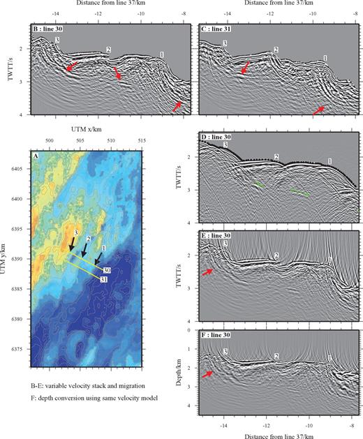
Median valley wall, fault related mid-crustal reflectivity. (a) Bathymetry of the south-western region of the work area contoured at 50 m intervals with the locations of profiles presented in (b–f) shown by solid yellow lines and the locations of identified fault associated seabed offsets shown by numbered black arrows. (b–c) FK migrated profiles muted above the seabed. Red arrows illustrate the strongest mid-crustal reflectors. The fault scarps (labelled 1–3) can be traced between adjacent profiles. (d–f) Line 30 where (d) shows the TWTT section, (e) shows the same data after FK migration and (f) the depth converted version of (e). Seafloor (black dots) and mid-crustal reflection (green crosses) TWTT picks have been shown in (d) for reference while the red arrows highlight the set of real events which can be mapped across multiple adjacent profiles. These events are interpreted as mid-crustal reflections associated with relatively steeping-dipping fault planes (e and f) and their more shallowly dipping extensions (b and c). See Figs 18, 19 and 20 for possibilities for the source of these events.
The green reflectors are observed to dip towards the ridge axis. To ascertain the true dip, profiles were migrated (Fig. 17e) and depth converted (Fig. 17f) using a velocity model (Fig. 18a) derived from 2-D finite difference forward modelling (Fig. 18b). The best-fitting model shows that the events are the result of multiple reflectors that appear to be located beneath the major inward-facing normal fault scarps that offset the seabed. The diffraction hyperbolae seen at the edges of the synthetic reflectors are not observed in the real data, which suggests that in reality these features do not terminate abruptly. For the example shown in Fig. 18, the three discontinuities dip at between 17° and 39°, with each being of the order of ∼500 m in length. The association of these reflectors with the seabed expression of faulting implies a link between the two. Several possibilities exist. The events may represent pre-existing surfaces rotated by subsequent faulting (Fig. 19), or they may themselves represent fault planes (Fig. 20).
Reflector geometry beneath median valley wall. (a) 2-D model containing three dipping linear crustal discontinuities (pink lines) used to calculate the stacked synthetic data in (b) which shows that the TWTT of the events closely matches that for the real data (green crosses). The numbers on all panels label the fault scarps as identified in Fig. 17. (c) Comparison of depth and dip of the modelled mid-crustal reflection events to the depth converted real data. Although the general agreement is seen to be reasonable, the dip of the events is not exactly matched.


Origin of dipping crustal discontinuities. Upper Panel: The location of discontinuities imaged on line 30 (red) relative to the seabed. The dashed lines, dipping at 55°, represent possible fault plane orientations which offset the seabed. Lower panels: Model A represents a flat, newly formed seabed within the median valley (grey: crust; blue: sea water). Two discontinuities are shown. The red discontinuity could reflect a sub-horizontal lithological boundary, while the green a dipping fault plane. Model B shows crustal deformation by faulting and the rotation of the fault blocks which comprise the median valley walls. Model C shows subsequent in-filling of intrafault block depressions (e.g. by later extrusive flows or debris). In Models B & C the orientation of the red and green discontinuities is shown. It would be expected that the green discontinuity would only be observed within one of the rotated fault blocks, especially since it is now relatively shallowly dipping. The red discontinuities now dip away from the ridge axis which suggests that the dipping seabed offset-related events observed on the seismic profiles are most likely fault related.
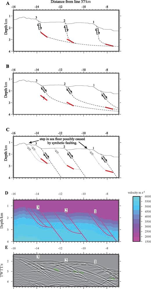
Three fault geometries that could cause the mid-crustal reflection events beneath the median valley walls. (a) Faults close to the surface dipping at 85°, which become listric at ∼2 km below the seabed where they form a common detachment surface. Solid red lines indicate the geometry of the reflection events from the 2-D modelling. (b) Faults close to the surface dipping at 55°, which become listric at ∼2 km below the seabed where they form a common detachment surface. (c) Large faults (shown by the black dashed lines) dipping at 55° extending to depth. Smaller synthetic faults, with a similar dip near the surface, but which become listric at depth, are shown in the footwall block of each fault as dotted lines. These synthetic faults may reflect internal deformation of the footwall block, and could be the origin of the smaller steps seen in the seafloor. (d) Velocity model with the proposed fault distribution shown in (c), incorporated as a set of discontinuities. (e) Stacked synthetic section from the model in (d) showing both seabed scattered energy and reflections from sub-seabed structures. The green crosses show the TWTT to the reflection horizons as seen in the real data (see Figs 16 and 17). The numbers in all parts label the fault scarps as identified in Fig. 16.
Fig. 19 illustrates how the orientation of two pre-existing discontinuities, or layer boundaries, might be affected by normal fault motion. It is clear that an originally horizontal discontinuity would not fit our observations. However, an originally steeply dipping discontinuity (e.g. an old fault surface) would rotate and dip towards the median valley. Observed event dips decrease towards the ridge axis, which would suggest that inner fault blocks may rotate more than older, outer fault blocks. The logical conclusion of this argument is that the interpreted fault-associated discontinuities are caused by a single, or system, of discontinuities that pre-dated all faulting activity as evidenced by fault scarps at the seabed.
Analysis of earthquakes originating along the Reykjanes Ridge (Fig. 21) shows focal mechanisms to have a strong normal component with nodal plane dips within the range 35°–55°. Only hypocentres shallower than 7 km below the seabed are observed. This is consistent with observations elsewhere on the MAR (e.g. Kong 1992; Barclay 2001) and suggests that the brittle-ductile transition lies at around this depth at the ridge-axis.
Recent earthquake locations within the RAMESSES study area. Grey dots show event locations obtained from the USGS catalogue (1976–2002), while ‘beach balls’ show fault mechanisms (double couple only) for larger events from the Harvard CMT catalogue. The majority of events lie within the median valley. The range of dips of normal nodal planes is ∼35–55°. The seabed bathymetry is shown for reference.
We have developed three models to test possible origins for the green events. Fig. 20 shows these models, all of which are based on the assumption that off-axis earthquake activity and fault systems result from normal faulting associated with extension along the spreading direction.
In Fig. 20 model A, the events originate directly from large offset, listric, block-rotating fault planes—which are imaged only at depth. We assume that no reflections are seen from shallower parts of the faults because the dip of the fault surface is too great. This model suffers from two major disadvantages. First, to match the geometry of the reflecting horizons the dip of the fault planes must be ∼80° immediately below the seabed. Secondly, in this model no faults propagate to depths greater than 2 km below the seabed. Both of these are incompatible with the earthquake data from the region. In model B, the scarps at the seabed again correspond to major inward-facing normal faults that become listric at depth, but in this case the reflectors are associated with the listric part of a fault plane which crops out at an adjacent escarpment. Although the fault plane dips do not exceed 55°, this model suffers the same disadvantage in that the fault planes do not propagate more than 2 km beneath the seabed.
It is possible that the depth of the brittle-ductile transition beneath the median valley flanks varies through time, with the stages of the tectono-magmatic cycle. In that case, the green reflectors may correspond to listric faults that during the current, relatively magmatic stage of the cycle sole out at a depth similar to the top of the axial crustal magma body. This does not preclude the possibility of the major faults extending to substantially greater depths, as indicated by the earthquake data, along parts of the ridge that are currently at a tectonically dominated phase of the cycle.
In the final model, C, the reflection events are not directly related to the large offset faults, but instead originate from low-dip portions of synthetic faults associated with the major fault systems. The synthetic faults may result from unloading and internal deformation of the footwall block due to fault motion associated with on-going extension. This model is supported by the observation of smaller seabed offsets further off-axis from the major seabed fault scarps.
To test model C, a finite difference model was created which represents the fault geometry as a set of discontinuities. The synthetic profile is shown in Fig. 20(e). Although this profile contains many arrivals which can be attributed to seafloor scatter (cf.Figs 2, 7 and 8), events matching the observed reflectors—including the absence of diffraction hyperbolae—are clearly seen.
We conclude that the green reflectors are directly related to major normal fault systems that form the walls of the median valley; and that only the sections of the faults with shallower dips are imaged. However we cannot resolve from our data whether these major bounding faults are listric, soling out at a depth of ∼2 km; or are planar faults extending deeper into the crust, but accompanied by smaller listric synthetic faults related to internal deformation of the footwall blocks.
5.5 Lower-crustal reflectivity beneath the ridge-axis (yellow)
Fig. 9 shows a series of deeper reflection events at ∼4 s TWTT, observed only on the profile along the AVR axis (grid line 37). This ‘intracrustal’ event is at a similar TWTT to a series of events observed on the original fourfold MCS data which were interpreted as peg-leg multiples from the AMC by Navin (1998). That interpretation was considered the most likely origin at the time, in the absence of multiple intersecting across-axis profiles, and was based on conversion of their along-axis wide-angle velocity-depth model to TWTT for direct comparison with the coincident RAMESSES I MCS data. However comparison with the results of scatter simulation using the ‘quick and simple’ approach (Fig. 9), shows that this event may instead be scattered energy from the seabed. We conclude that it is more likely that neither the yellow event in this study, nor the peg-leg multiple reported by Navin (1998), correspond to real intracrustal reflections.
5.6 Summary
Four types of reflection events have been consistently imaged throughout the survey area. Fig. 22 shows a summary 3-D view of these.
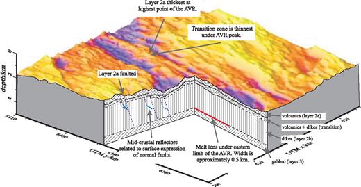
3-D model summarizing the main reflectors identified in this study. The seabed topography of the RAMESSES work area is cut-away to reveal the intracrustal geological structures imaged with the MCS data. Arrows and corresponding text boxes each show separate features, and the supporting evidence for each. Comparison of this model with Navin 's (1998) wide-angle velocity-depth model shows that there are significant similarities where similar structures are imaged.
- 1
The shallowest event to be imaged is interpreted as representing the base of layer 2A—the extrusive part of the oceanic crust. Although not imaged as a primary reflection, it is observed on all profiles and can be mapped consistently throughout the entire survey area, using the preferred variable velocity model (Fig. 12a) to convert TWTT into depth. The base of layer 2A lies between ∼130 and 520 m below seafloor (bsf), and is found to be deepest beneath the shallowest bathymetric point of each AVR. The base of the layer is offset by the numerous ridge-parallel faults that form the median valley walls.
- 2
Beneath the AVR a horizon is imaged up to ∼1000 m below the base of layer 2A. At its shallowest, which is also the shallowest topographic point on the AVR, it is almost coincident with the base of layer 2A where the latter is thickest. This horizon is interpreted as the base of a transition zone comprising mixed volcanic extrusives and sheeted dykes. The thinnest part of this layer is interpreted to reflect the region of most recent melt flux to the seabed, building the highest peak in the AVR topography. It is only seen in close proximity to, or directly beneath, an AVR and has not been observed off axis.
- 3
Within the median valley two sets of melt event are imaged, both of which are interpreted as reflections from the top of a melt body within the crust. The first set of events occurs beneath the axes of each AVR. The second set is imaged beneath the two offset basins that separate the AVRs. The two sets of reflectors are interlinked by a lower amplitude reflection event imaged in the across-axis profiles. Both sets of melt reflectors are at depth of ∼2.5 km below the seabed, consistent with the depth inferred from the wide-angle velocity model of RAMESSES I (Navin 1998).
- 4
The final class of reflection events is imaged under the flanks of the median valley. Their individual locations correlate closely with prominent escarpments on the seabed that form the median valley walls. These reflectors are clearly associated with major extensional fault systems, but their precise geometry and origin remain unclear.
In the next section the individual observations from this survey will be combined and integrated with the other results of the RAMESSES project to date, to develop a 3-D model of crustal structure, magmatic accretion and tectonic processes that operate within the median valley of this slow-spreading mid-ocean ridge.
6 Interpretation and Model of Crustal Accretion
The combined analysis and interpretation of the various geophysical data sets acquired within the RAMESSES I project led to the recognition of an AVR as an integral component of the spreading system, with an independent and intermittent source of magma from the underlying mantle into the lower and mid-crust driving independent tectono-magmatic cycles. By seeking to image the along-axis variability in crustal structure beneath the RAMESSES AVR and its neighbours, the RAMESSES II project aimed to test this hypothesis and to explore what further implications it carries for crustal accretion in general and for the relationship between tectono-magmatic cycles and ridge segmentation in particular. We pose a series of questions which we shall now address using the results of data analysis and interpretation from all elements of the RAMESSES studies.
First though we assess two specific aspects of the geometric relations between the reflecting horizons identified in the previous section. The first of these is the AMC reflector. We need to explain the existence of an AMC reflector beneath the length of the RAMESSES I AVR, beneath the offset basins to the northeast and southwest of it, and beneath the neighbouring AVR to the north.
MacGregor (1998) estimated that the magmatic phase of each cycle occupies no more than 10 per cent of the cycle time; with the amagmatic phase accounting for at least 90 per cent of the time. The implication of the widespread distribution of AMC reflectors in this study is that at the start of a cycle, melt influx to the crust must occur along-axis over a distance substantially greater than that of a single AVR (e.g. Peirce 2005). Hence tectono-magmatic cycles drive the accretion process not at single isolated AVRs, but over a longer length of the ridge—corresponding to a lower order of segmentation than a single AVR. Secondly the existence of AMC reflectors beneath the offset basins indicates that the distribution of AVRs along-axis varies through time: AVRs have a life cycle of inception, activity and extinction, before being superseded by new AVRs that are generally centred on different along-axis locations. If this is the case the AVR within the RAMESSES I study area—although recently rejuvenated by a new tectono-magmatic cycle—may be at a relatively mature stage of its overall life cycle. In contrast the offset basins correspond to sites of the earliest stages of formation of the next generation of AVRs. These conclusions fit the model of Peirce (2005), who explain the relationship between tectono-magmatic cycles and AVRs in the context of time-varying melt supply to a second-order segment comprising several AVRs. A magmatic segment length longer than a single AVR would be consistent with typical second-order segment lengths of 50–80 km along the MAR elsewhere in the North Atlantic, and with numerical models of mantle upwelling that predict length scales of the order of 100 km for the spacing between adjacent upwelling regions (e.g. Parmentier & Phipps Morgan 1990). Gardiner (2003) and Peirce (2005) have shown on the basis of residual mantle Bouguer anomaly (RMBA) modelling that thickened crust is present beneath the offset basins, consistent with the conclusion that these features mark the along-axis sites of newly forming AVRs at the very start of their life cycle.
The second key set of relationships relates to the distribution of the major fault systems and the relict AVRs identified from variations in layer 2A thickness. The seabed bathymetry (Fig. 1), the faulting pattern observed on each profile (e.g. Figs 7 and 17) and the layer 2A isochron (thickness) and major fault trace map (Fig. 15d), show that the main seabed-offsetting faults—which can be traced across multiple profiles—have a range of orientations between AVR-parallel and ridge-parallel. Within the median valley, close to the AVRs, the faults tend to be approximately AVR-parallel. Further from the axis, the faults are more likely to be aligned parallel to the overall ridge trend, as noted by Searle (1994). It is these faults that tend to form the large escarpments that correspond to the median valley walls. However, it is unusual for these major fault systems to cut through relict AVRs—instead, the relict AVRs tend to be situated between major faults, so that they sit within the major fault blocks rather than being broken up by them.
6.1 Key questions
Q1: Is there (at certain stages of the tectono-magmatic cycle) a single magma body within the mid-to-lower crust that extends for more than one AVR, along a ridge-parallel (AVR-oblique) direction and feeds more than one AVR?
No. The distribution of axial melt lens reflection events in both the RAMESSES II MCS and the RAMESSES I wide-angle data sets indicates that each AVR is underlain by a separate magma chamber within the crust (Fig. 15b). Navin 's (1998) across-axis velocity model shows that this magma chamber contains approximately 20–40 per cent partial melt, which is periodically refreshed from the mantle on the order of every 20 000–60 000 yr (MacGregor 1998). The crust is thickest beneath the shallowest AVR topography, as evidenced by the along-axis velocity model of Navin (1998), free-air gravity anomaly modelling (Navin 1998; Peirce & Navin 2002; Gardiner 2003; Peirce 2005) and a residual mantle Bouguer anomaly low (Gardiner 2003; Peirce 2005). Layer 2A is also thicker at the centre of the AVR, as evidenced by a magnetic intensity high (Fig. 15a; Lee & Searle 2000; Gardiner 2003; Peirce 2005) and by the seismic data in this study. The AMC reflector reaches its minimum depth below the seafloor at the AVR centre (Fig. 15b and Topping 2002). All of this indicates that each AVR is fed by a separate melt supply located beneath the AVR centre.
Q2: Is there an intermittent source of melt within the mantle which extends for several AVRs along-axis in a ridge-parallel, AVR-oblique direction, and which is tapped in different locations and at different times by multiple AVRs spaced along it?
There is a range of crustal through to mantle based evidence to support this concept. Heinson (2000) used MT data to show that the melt source region lies at a depth of 50–100 km below sea level and that accumulation and transport to the crust is rapid and episodic, there being no evidence from the MT data of any clear conduit or connection between the mantle melt source and the crustal magma body. Peirce & Navin (2002) showed from RMBA modelling that magma delivery from the mantle to the crust takes place along the ridge trend and that individual AVRs tap this supply at the crustal level, initiating a tectono-magmatic cycle and accommodating crustal accretion. Continued amagmatic spreading later in the cycle is accommodated by AVR-parallel faulting and fracturing. The RMBA exhibits two trends. A ridge-parallel long-wavelength negative anomaly encompasses several adjacent AVRs. Superimposed on this are shorter wavelength lows associated with, and trending along, each AVR. Gardiner (2003) and Peirce (2005) extended this modelling to incorporate the relative ages of AVRs and spreading rate calculations. They conclude that a second-order ridge segment at this location on the MAR is ∼70 km in length and comprises multiple AVRs, with the AVR at the centre of the second-order segment being the oldest and most topographically robust, and AVRs heading towards segment ends being progressively younger and shorter. In other words, AVRs are ‘plumbed’ independently at a crustal level, but sit astride a longer-wavelength melt supply from the mantle which feeds several AVRs over a distance of ∼70 km along the ridge trend.
Q3: Is an AVR a whole-crustal phenomenon, with the AVR axis constructing the entire crust? Or is it simply a layer 2 phenomenon? In other words, is an AVR underlain by an intermittent axial magma chamber which runs along its length at mid-lower crustal level and can redistribute melt along-axis within layer 3 as it forms, or is melt transport along-axis confined to sheeted dykes within layer 2, with the AVR itself being merely the expression of lateral melt transport at this level from a deeper magma body located beneath the AVR centre?
Several pieces of evidence point towards AVRs being a whole crustal phenomenon. The presence of an AMC reflection event along the entire length of each AVR surveyed implies a crustal magma chamber within layer 3 aligned with the AVR axis. The depth bsf of this reflecting horizon (Fig. 15b) and both the along- and across-axis wide-angle velocity-depth models (Navin 1998) suggest that although the melt supply from the mantle to the crust is at least partly focused beneath the AVR centre, this melt is redistributed along-axis at a lower crustal level before either solidifying to form the lower crust, or escaping upwards (and in some cases erupting) to form the sheeted dyke complex and extrusive rocks of layer 2 and the seabed expression of the AVR. The RMBA modelling of Gardiner (2003) and Peirce (2005) for multiple adjacent AVRs at this location on the MAR shows that each has a low density region within layer 3 beneath the AVR centre, and each shows thinning of layer 2A and of the crust as a whole towards AVR tips. The results of Topping (2002) and this study also show layer 2A to be thickest at the AVR centre, implying an enhanced melt supply.
Q4: Is the tapping of the along-axis mantle melt source confined to point locations coincident with AVR centres, or does melt arrive in the crust along the entire length of an AVR?
The evidence that supports AVRs being a whole crustal phenomenon also supports melt supply into the crustal magma chamber being an AVR-centred process. The apparent absence of a mixed zone of dykes and extrusives at the AVR centre, beneath the shallowest bathymetric point, also supports the point-source, AVR centre melt supply model. However the presence of AMC reflectors beneath offset basins suggests that new AVRs can be initiated at sites along the ridge trend that do not currently coincide with AVR centres, but which will in time grow into new AVR systems by means of melt redistribution within the crust along the spreading-orthogonal, AVR trend.
Q5: Are the along-axis sites of melt injection to form AVRs fixed, or can AVRs form in new locations along axis?
This has already been considered in the previous paragraph. The evidence is that AVRs are not fixed in location at specific points along the ridge axis, but can and do form wherever melt accumulates within the crust along the ridge trend; and that its arrival initiates a new tectono-magmatic cycle, and the growth or rejuvenation of an AVR. Further support for this lies in the identification of intact relict AVRs and accompanying offset basin pairs, asymmetrically located within the median valley (Fig. 15). Gardiner (2003) and Peirce (2005) have noted that over timescales of less than ∼1.4 Ma, this part of the Reykjanes Ridge is spreading asymmetrically. A natural consequence of this is that overtime, AVRs progressively migrate off-axis in the direction of slower spreading. For the currently magmatically active AVRs, this is in a westward direction from the ridge axis. Gardiner (2003) and Peirce (2005) have also noted that the focus of the short wavelength RMBA low associated with each AVR is also systematically offset from the AVR in the slower spreading direction, suggesting that the most recent melt influx to the crustal magmatic system has occurred along the ridge-trending focus of upwelling (in an across-axis sense), rather than specifically beneath the across-axis centre of an existing AVR. These observations lead to the conclusion that each AVR undergoes a series of tectono-magmatic cycles as part of its life cycle, until it has migrated sufficiently far to one side of the median valley by asymmetric spreading that it is too far from the ridge-trending focus of melt delivery to receive further melt influxes. At this point the AVR comes to the end of its life span and a new AVR is ‘born’ elsewhere, more centrally within the median valley. The current offset basins are sites where this is happening now.
Fig. 23 shows the current locations of active AVRs, offset basins, and the relict AVRs that can be most reliably identified using a combination of swath bathymetry and layer 2A thickness data and that have been rafted off-axis largely intact. The across-axis spacing of these relict AVRs is typically 4–7 km, corresponding to a time interval of 0.4–0.7 Ma, implying that the life span of an AVR is of this order. Changes in the direction of asymmetric spreading over timescales of no more than 2.4 Ma allow for symmetrical spreading of the ridge as a whole over the longer term.
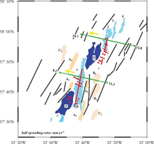
Major volcanic and tectonic features of the study area. Currently active AVRs are shown in solid green–blue, numbered from 1 (the RAMESSES I AVR) to 4. Extinct AVRs, reliably identified from combined swath bathymetry and layer 2A thickness variations (see Figs 1 and 15), are outlined and hatchured in orange. Green arrows show asymmetric spreading half-rate vectors while yellow arrows show the resulting direction of AVR migration (towards the slower spreading plate). Offset basins α and β are shaded dark blue. Major fault lineations, indicating the escarpments formed by normal faults that create the median valley walls, are shown by solid black lines. The locations of melt lens reflection events observed beneath AVRs and offset basins are shown in red.
Q6: Do several AVRs constitute a single second-order segment, with some synchronicity of the tectono-magmatic cycle along the second-order segment?
The implication of this question is that AVRs are third-order segments in the terminology of Macdonald (1982). The relative dating of AVRs based on their bathymetric expression, crustal structure and magnetic and gravity anomalies by Gardiner (2003), Peirce & Navin (2002) and Peirce (2005) suggest that AVRs are independent entities at the crustal level, but that they are interconnected at the mantle level through their longer time frame melt supply. This supports the hypothesis that several AVRs comprise a second-order segment, and that such a segment can be defined by the wavelength of melt delivery from the mantle. In Peirce 's (2005) model, all of the AVRs in each second-order segment experience a series of tectono-magmatic cycles, but their relative phase in each cycle is determined primarily by their along-axis distance from the focus of melt delivery to the shallow mantle beneath the centre of the second-order segment.
At the second-order segment level, our observations, results and models for the Reykjanes Ridge can be compared to similar results from both slow- and fast-spreading ridges. For example, Dunn 's (2005) observations at 35°N on the MAR lead to a similar conclusion that mantle melt supply is focused towards second-order segment centres and that this melt is redistributed within the crust at lower crustal levels. Their model also features anomalously thick crust and a low-velocity anomaly at the centre of a second-order segment. In addition, they interpret observed seismic anisotropy in the lower crust as reflecting melt-filled dykes which channel melt not only from the mantle into the crust but also within the crust. The trend of these dykes is observed to be rotated ∼30°–40° away from the ridge-parallel direction as a consequence of the ∼40° difference between the ridge trend and the spreading direction. A similar setting exists at the Reykjanes Ridge, and Peirce (2005) conclude that such focused melt delivery and redistribution controls the observed third-order segmentation pattern and the timing and relative duration of tectono-magmatic cycles of accretion.
Similarly, at 9° 30′N on the fast-spreading EPR, Dunn (2000) observe similar patterns and wavelengths in along-axis velocity anomalies between the upper crust, lower crust and uppermost mantle, from which they infer that melt supply is currently focused along-axis beneath the central third-order (∼13 km) segment—bounded by two devals—of a much longer (∼100 km) second-order segment. As part of their study they used seismic anisotropy to investigate mantle flow beneath the ridge-axis. They found no evidence for diapiric mantle flow, which led them to conclude that, at 9° 30′N, mantle flow and melt migration patterns are effectively decoupled. In other words, at this fast-spreading ridge mantle flow is essentially 2-D, but melt migration in the shallowest parts of the mantle is inherently 3-D.
Thus our conclusions, in terms of the along-axis focusing of melt supply beneath second-order segment centres, are consistent with other observations from both the fast-spreading EPR and other sites further south on the slow-spreading MAR. However, in this case, the combination of oblique spreading and subdued median valley topography—which assist both in sub-seafloor imaging and in the identification of along-axis segmentation patterns—with the recognition of cycles of tectonic and magmatic activity and the availability of multiple data types (potential field, swath bathymetry, deep-towed side scan images, wide-angle and multichannel reflection seismic, MT and CSEM), have allowed us to go further. For the first time we have been able to link temporal cycles, with two different periods, to segmentation patterns at both second and third order.
6.2 The model—nested cycles of accretion and orders of segmentation
The answers to the above six questions, each supported by extensive evidence from a wide variety of geophysical techniques and approaches, leads to the following summary model for second- and third-order segmentation, for the birth, life and death of AVRs and for the relationship between temporal and spatial aspects of accretionary processes operating within the crust and the upper ∼100 km of the mantle. All of the evidence from this and the other RAMESSES studies points to an interrelated set of nested cycles of accretion operating on different geological timescales, and nested orders of segmentation operating on different along-axis wavelengths.
Cycle 1:The tectono-magmatic cycle
This shortest time frame cycle comprises repeating patterns of AVR rejuvenation, volcanism and magmatic crustal growth followed by tectonic dismemberment and amagmatic extension. Each cycle lasts typically 20 000– 60 000 yr. The magmatic phase occupies no more than 10 per cent of this, while the amagmatic phase occupies at least 90 per cent. This cycle represents the independent melt refresh rate to the crustal magmatic system beneath each AVR.
Cycle 2:Asymmetric spreading and accommodation within the median valley
After an AVR forms it gradually migrates towards the more slowly accreting plate over several tectono-magmatic cycles. This migration intrinsically limits its life span. Eventually a new AVR forms, typically within an offset basin between AVRs of the previous generation. Old, extinct AVRs are often preserved more or less intact, preferentially on the slower spreading side of the median valley. The sense of asymmetry in spreading rate reverses from time to time, to accommodate the symmetrical spreading observed over longer geological time frames (>2.4 Myr in this case). Each newly forming AVR tracks across the median valley in the direction of slower accretion, which may be in the opposite sense to its predecessor. This is a longer cycle of the order of 0.5–0.7 Myr. For the AVRs in the RAMESSES study area, this implies that an AVR might expect to go through a number (perhaps 10–20) of tectono-magmatic cycles between inception and extinction.
Third-order Segments:Axial volcanic ridges
AVRs constitute third-order segments, each being underlain at the height of the magmatic phase of its tectono-magmatic cycle by an independent crustal magma body. The latter redistributes melt both at upper crustal and at mid-to-lower crustal level along the AVR axis, to generate new oceanic crust.
Second-order Segments:Segmented magma supply from the mantle
Several AVRs over an along-axis distance of the order of 70 km are linked by deeper-seated processes that lead to synchronicity of their tectono-magmatic cycles. Within a second-order segment, AVRs tend to be largest, most robust and underlain by the thickest crust near the segment centre; and to be progressively shorter and less robust towards the segment ends. The onset of the magmatic phase of a tectono-magmatic cycle appears to occur first at the centre of a second-order segment, and to progressively affect AVRs at later times towards the segment ends.
This model can be tested by geochemical analysis and absolute dating of accurately located samples, distributed systematically both along- and across-axis at existing and relict AVRs. If the offset basins are currently the sites of the inception of a new generation of AVRs, they should be underlain by thicker crust and by a corresponding magma chamber, both of which can be imaged by wide-angle seismic means.
7 Conclusions
In this study we have presented the analysis of a grid of 37 multichannel reflection profiles acquired as part of the RAMESSES project. The results and conclusions have been integrated with the results of all of the RAMESSES data sets, to reveal a 3-D image of crustal structure beneath a magmatically active axial volcanic ridge segment and its neighbours. Based on this we propose a model of linked ridge segmentation and cyclic crustal accretion. Our main findings are summarized as follows.
7.1 Processing of multichannel reflection profiles from mid-ocean ridges
Extensive seismic data processing tests showed that, in this mid-ocean ridge setting, the simplest approach to data processing generally gave the best results. In particular, CVSs can be targeted to particular horizons and events. Variable velocity stacking with either NMO or pre-stack DMO and migration resulted only in minor improvement.
At mid-ocean ridges, particularly slow-spreading ridges, seabed scattering is a significant problem largely because of out-of-plane energy, and neither 2-D migration nor 2-D pre-stack DMO can prevent this from masking intracrustal events. A fully 3-D data set and fully 3-D pre-stack processing methods, able to deal with the steep dips and severe lateral velocity gradients, are in principle the only way to fully tackle this problem. However, experience to date has shown that even this approach does not solve the problem entirely.
Two approaches to minimizing and predicting seafloor scattered signals show that comparable results to full 3-D acquisition and processing can be achieved by simple predictive modelling, ground-truthed against full wavefield pre-stack simulations, if the models are used to distinguish genuine intracrustal events of geological origin from seafloor scattered noise.
7.2 Upper crustal structure
- 4
The thickness of the extrusive part of the oceanic crust, layer 2A, is greatest at AVR centres, and declines both off-axis from the AVR and along-axis towards AVR ends. Both AVR-parallel and ridge-parallel trends are observed, with the pattern of on-axis layer 2A thickness variation preserved beneath relict AVRs rafted off axis. The central anomaly magnetic high in general follows the ridge trend, but shorter wavelength (AVR scale) magnetization intensity highs coincide with areas of thicker layer 2A—both for currently active AVRs and in some cases for relict AVRs that have now been rafted off-axis.
- 5
The AVRs in this study are spreading asymmetrically with faster accretion towards the east. This leads to gradual westward migration of the AVRs within the median valley. This process ultimately leads to AVRs becoming extinct, to be superseded by a new generation of AVRs.
- 6
Ridge-parallel faults tend to form in older crust near the edges of the median valley. AVR-parallel faults are more likely to form within the median valley. The major bounding faults of the median valley tend not to cut relict AVRs—so that old extinct AVRs tend to be preserved more or less intact within the major fault blocks, and to be rafted off-axis intact and in the direction of slowest spreading.
7.3 Mid-crust and below
- 7
Each AVR is underlain by a mid-lower crustal magma chamber extending along most of its length and aligned orthogonal to spreading direction. Crustal thickening is observed at AVR centres, implying magma supply into the crust occurs primarily here, while a longer-wavelength supply from the mantle is aligned along the overall ridge trend.
- 8
AVRs are a whole crust phenomenon, and not merely a consequence of melt redistribution by sheeted dykes within layer 2 of the oceanic crust.
7.4 Melt beneath offset basins
- 9
Mid-crustal melt bodies are present beneath the two offset basins (α and β in Fig. 23) southwest and northeast of the RAMESSES I AVR. These will develop into new AVRs, and we would expect that overtime the sense of spreading rate asymmetry will reverse. If the inception of new AVRs is accompanied by reversals in the sense of asymmetric spreading, this will tend to lead to extinct AVRs being alternately rafted off-axis in opposite directions, favouring their preservation.
- 10
The east–west spacings of relict AVRs and basins—evidenced by both bathymetry and layer 2A thickness—is of order 5–7 km, corresponding to a cycle time of order 0.5–0.7 Myr at the average spreading half-rate here of 10 mm a−1.
7.5 The proposed model
- 11
The integrated interpretation of all data sets acquired as part of the RAMESSES projects, together with other data acquired along the entirety of the Reykjanes Ridge, has enabled us to propose a model for crustal accretion at this part of the slowly and obliquely spreading Reykjanes Ridge which links two orders of along-axis segmentation with two nested cycles of AVR inception, activity and extinction, and tectono-magmatic seafloor spreading. The model is summarized in Section 6.2 above.
Acknowledgments
We would like to thank the officers and crew of RRS Discovery, the sea-going technical staff of the United Kingdom Ocean Research Services (UKORS) and the members of the scientific party of cruise D235c/98. This research was supported by the Natural Environment Research Council via a research grant (GST02/1500), ship time and PhD studentships (CJG, ST), together with a research grant from the University of Durham. The phase screen modelling code was kindly provided by Richard Hobbs. Figures were created using the Generic Mapping Tools of Wessel & Smith (1995) and Seismic Unix. Finally, we thank three anonymous reviewers for their comments which greatly improved the clarity of this paper. Further information can be found on the RAMESSES www home page ().
References
