Comparison of methods to model the gravitational gradients from topographic data bases Free

Summary

1 Introduction

Since the time that it could be measured, more than 100 years ago (Szabo 1998), the gravitational gradient has been the subject of study in physics, geophysics, and geodesy, even though its measurement is far from easy and the instrumentation must be exquisitely precise to be of any use. Eötvös's extraordinary yet cumbersome static gradiometer, in fact, was quickly replaced in the 1930's and 1940's by the portable relative gravimeter when the latter achieved sufficient accuracy for geophysical exploration. Requiring only a fraction of the time to make a measurement, the gravimeter became the stalwart of both geophysical and geodetic gravimetric surveys. Gradiometers experienced a resurgence, at least on paper initially, with the advent of satellites (specifically, planetary probes) since only the curvature of the gravitational potential field can be sensed on a freely falling body (such as a satellite). To date, no gradiometer has managed to fly in space as other modes of gravitational field measurement by satellites (precise orbital tracking) proved less expensive and were already at hand. Airborne gradiometry, analogously, was considered in the 1970's to solve the problem of inseparability of inertial and kinematic acceleration that besets any gravimeter (or accelerometer) on a moving platform (the basic physical principles are identical to the case of the satellite). Again, the development of other technology thwarted the gradiometer's rightful place in moving-base gravimetry. GPS positioning quickly developed to a level of precision that kinematic accelerations could be determined independently with commensurate accuracy.

Gradiometer technology continued undaunted with the promise of eventual deployment in space; and, after two potential missions were abandoned, an Earth-orbiting gradiometer is now firmly scheduled for launch in 2007 (Drinkwater 2003). Near-surface deployments also continued since the partially successful demonstrations in the 1980's (Jekeli 1988, 1993). Recent successes in geophysical exploration (van Leeuwen 2000) have once again brought the gradiometer to the fore, and new technology developments associated with atom interferometry (McGuirk 2002; Jekeli 2004) promise accuracy as well as efficiency in instrumentation (thus reducing cost and increasing resolution in the measurements).

The utility of gravitational gradiometer (as opposed to the gravimeter) is well known (e.g. Heiland 1940; Hammer & Anzoleaga 1975; Dransfield 1991; Marson & Klingele 1993). Being more sensitive to the near surface density contrasts and with higher acuity, the gradiometer should be better able to discern mineral deposits and small-scale, near-surface geologic features. Moreover, gradient-measuring instruments generally provide multiple components of the full gradient tensor; and, in principle, measuring the full tensor yields five independent characteristics of the field compared to only three provided by the gravitational vector.

As with any sensor, its full potential can be realized best if the signal is nulled (or, at least substantially reduced) with prior information, so that the sensed quantity is a small residual to an otherwise computed and known field. We already have quite detailed and accurate models of the Earth's gravitational potential field (e.g. EGM96, Lemoine 1998), which imply a corresponding gradient field. However, the spatial resolution of such global models is limited (to about 50 km half wavelength for EGM96); and, while local gravimetric surveys might yield models with a resolution as fine as a few kilometres, at 100 m altitude, 90 per cent of the gravitational gradient signal resides in wavelengths shorter than several hundreds of metres (after accounting for the Earth's ellipsoidal bulk). Closer to the topographic surface, the signal is even more sensitive to the very near masses (which also contributed to the downfall of the gradiometer in favour of the gravimeter that is less overwhelmed by close, possibly non-permanent density contrasts). Thus, very detailed models of the known field should be constructed for gradiometric surveys.

Aside from the gradients implied by global and local gravimetric models, finer resolution can be obtained from the effect of the visible topography, since elevation data generally have higher resolution than gravity data. Toward this end, a number of computational algorithms have been developed based on a planar approximation of the height reference surface and a presumed density within the topographic masses. We adopt these approximations with the objective of evaluating the methods in terms of their relative precision and efficiency. The larger question of how much of the topographic signal is already contained in global and local gravitational models, while not addressed here, is assumed to leave unchanged the essential conclusions obtained here.

Analyses of gradient models from topographic data have been conducted in the past. For example, Tziavos (1988) and Schwarz (1990) considered methods exclusively based on Fourier transform techniques (also analyzed herein).

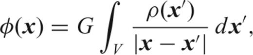
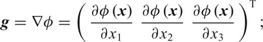
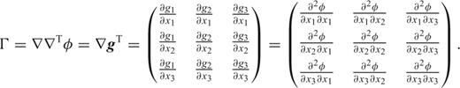
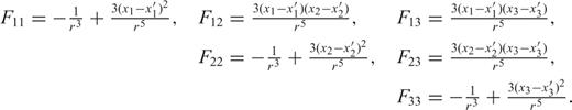
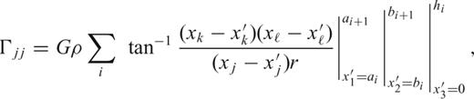
2 Gravitational Gradients

The following eq. (1) expresses the (scalar) gravitational potential at x due to a continuous mass distribution over volume, V, with density function, ρ(x′).

1

where G is Newton's gravitational constant and dx′≡dx′₁dx′₂dx′₃. The gravitational acceleration vector is the first-order gradient of the (scalar) potential field:

2

and, the gravitational gradient tensor comprises the second-order derivatives of the potential:

3

The gradient tensor is symmetric, and its trace is a function of local density according to Poisson's equation: ∇²φ (x) =− 4πGρ (x). Thus, if the density is known (e.g. it is zero), the gradient tensor expresses 5 independent gravitational characteristics of the field, any two diagonal components and the three off-diagonal components. However, there is greater interpretative information in the following five quantities: the vertical–vertical gradient, Γ₃₃; the differential curvature, Γ_C, of an equipotential surface, the direction of minimum curvature, α_C, given by:

4

and the horizontal gradient of vertical gravitation, Γ_H, being defined as the magnitude of a 2-D vector that has direction, α_H; the latter are given by:

5

Further elaboration on these quantities may be found in (Heiland 1940). The authors know of no shortcut to evaluate the horizontal gradient or differential curvature from mass models other than to compute first the tensor components. Thus, the comparison of methods addresses only the latter.

3 Gradient Models

The computational methods are all based on forward modelling of the gravitational gradients, where the density distribution is assumed to be known, specifically, ρ (x′) = constant; however, this is not a strict requirement in all methods, as indicated later. The boundary of the volume, V, is assumed known to some extent, fully for the theoretical developments, but only at discrete points for practical implementations. Applying the definition (3) to formula (1), we must evaluate the following integrals:

6

Analytic expressions for these integrals are possible for certain simple boundaries of V, specifically boundaries that are (closed) polyhedra, or composites thereof. Other simple surfaces, such as the sphere and ellipsoid also admit to analytic expressions for the potential, and hence its derivatives.

We consider the problem of determining the gravitational gradients from near-surface terrestrial masses. The reference surface for the terrestrial heights is assumed to be a plane. Hence, with a local Cartesian coordinate system, V is bounded by the (horizontal) (x′₁, x′₂)-plane, by planes perpendicular to this plane (which thus restrict the integration to an area, A, in the (x′₁, x′₂)-plane), and by an arbitrary surface, x′₃=h(x′₁, x′₂), representing the terrestrial surface. We write:

7

where, with r²= (x₁−x′₁)²+ (x₂−x′₂)²+ (x₃−x′₃)²,

8

The integrals of F_jk with respect to x′₃ are easily derived with a change of variable to α by: tan α= (x₃−x′₃)/s, where s²= (x₁−x′₁)²+ (x₂−x′₂)². Letting h≡h(x′₁, x′₂), we have

9

It is readily shown that the functions, T₁₁, T₁₂, T₂₂, and T₃₃ are not singular at the origin, s= 0, as long as x₃ >x′_3,max. Their limiting values at s= 0 are shown in eq. (9) for purposes of numerical evaluation (see also Fig. 1 that illustrates these functions for a typical set of h values). It is noted that eq. (7) with expressions (9) could as well be used if the density function is variable in the plane and is constant over intervals in the vertical.

Figure 1

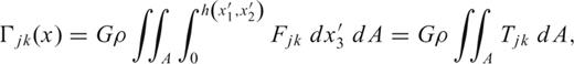
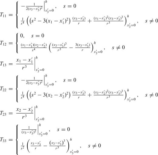
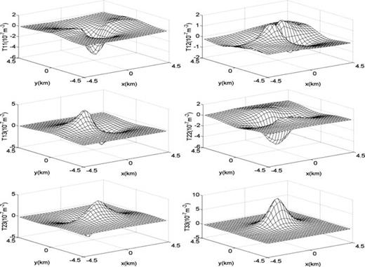
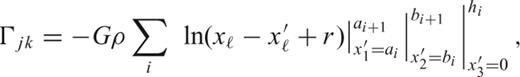
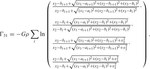
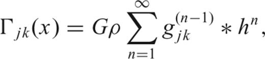
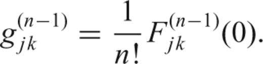
Kernel functions, T_jk, for a typical topographic function, h.

Open in new tabDownload slide

In practice the surface, x′₃=h(x′₁, x′₂), is known only approximately from a collection of data that represent measurements of heights at discrete points, or averages over intervals. From these one can construct a finite element model of the topographic masses using spline functions that approximate the bounding surface. Such splines are piecewise continuous polynomials of order, n= 0, 1, 2, …, where n= 0 represents a basis set of step functions. It can be shown that analytic expressions for the corresponding gradients exist only for n= 0, 1. For higher orders, the expressions involve elliptic integrals, which must be evaluated numerically. Often the data are arranged on a regular rectangular grid, so that for the case, n= 0, the integrals (7) are sums (over index, i) of gradients due to right, rectangular prisms with flat tops, given by the following formulas (e.g. Dransfield 1991; however, those given here are simpler; see also Forsberg 1984):

10

11

where in each case the index set, {j, k, ℓ}, is a cyclic permutation of {1, 2, 3}; for example,

12

Again, an obvious generalization holds if each right, rectangular prism has its own constant density.

For n= 1, representing a polyhedron, Petrovic (1996) and Tsoulis & Petrovic (2001) have derived comprehensive formulas for the potential and its first and second derivatives. Rather than repeating these formulas, which include several special cases that avoid singularities, we refer to the documents (ibid.) where they are derived and note only that our application is limited to the case where the topographic surface is triangulated by the given height data. Each triangle-topped prism may have a different density, but we assume a constant value as before. Fig. 2 illustrates the geometry for the two prism methods.

Figure 2

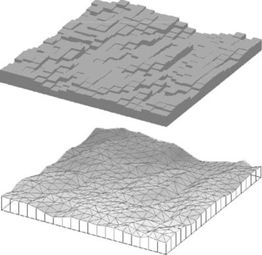
Geometries of rectangular (top) and triangular prism (bottom) representations of the topographic masses.

Open in new tabDownload slide

Instead of approximating the topographic surface by a simple spline function, one may choose to approximate the integrals over A numerically. This differs from the previous case in that now the function, T_jk, is approximated by splines, rather than just the height function, h. In other words, we integrate analytically in the vertical direction (constant vertical density). A standard numerical method is the rectangular rule, which approximates eq. (7) according to:

13

where for a regular rectangular grid, ΔA_i=Δx′₁Δx′₂. The numerical integration of eq. (7) with respect to a triangulation of the domain is analogous to the trapezoidal rule and is given by

14

where ΔA_i is the area of the ith triangle with corners represented by (i1, i2, i3). The generalization of the numerical integration to density functions that are variable in the horizontal plane has already been mentioned.

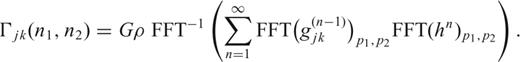
All of these methods may be computationally too intensive if many gradients are needed in an area and the height data set is large. One can employ Fourier transform techniques to reduce the number of computations significantly provided the height data are on a regular Cartesian grid and the computation points are on that same grid. The following two algorithms take advantage of the fast Fourier transform (FFT).

The first method is analogous to Parker's (1972) method that transforms the potential, eq. (1), into the frequency domain, applies well-known relationships between the spectral components of the gradients and the potential, and subsequently transforms the spectra of the gradients back to the space domain. Denoting by ℑ the continuous (2-D) Fourier transform operator with respect to horizontal coordinates, (x₁, x₂), we have from eq. (1):

15

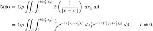
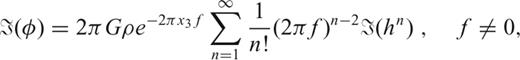
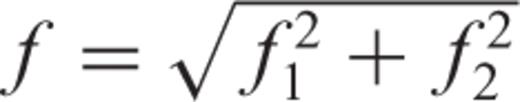where (f₁, f₂) are frequency coordinates corresponding to the spatial coordinates, (x₁, x₂), and where . Integrating eq. (15) with respect to x′₃, we find that

16

A series expansion of the exponential in eq. (16) leads to

17

provided that A= (−∞, ∞) × (−∞, ∞). However, since A, in practice, is a finite region, eq. (17) is an approximation. Also, we assume that the Fourier transforms of the powers of h exist, which, in the continuous case, constrains their measure (size) over the plane. These constraints change when we consider discrete approximations. Clearly, ℑ (φ) is singular at the origin, which is a property of the potential in planar approximation (the Newtonian potential of an infinite flat slab does not exist).

The relationships in the frequency domain between the potential and its second-order derivatives are given by (Jekeli 2003):

18

where

19

We see that the Fourier transforms of the gravitational gradients do not have a singularity at the origin:

20

and, we finally have

21

Note that this method requires a constant height for the evaluation points. The density was taken as constant for simplicity, but could be allowed to vary laterally, in which case the inner Fourier transform would be applied to ρhⁿ. The application of the Fast Fourier Transform on the right-hand side is discussed after developing the alternative formulation of the gravitational gradients as series of convolution integrals.

Indeed, the second Fourier transform method (Forsberg 1985) is based on the convolution theorem in spectral analysis, where the convolution is calculated more efficiently if it is first transformed into the frequency domain where it becomes a product. In order to implement this technique, the gradients, given by the left-hand side of eq. (7), are written as series of (continuous) convolutions, each having the general form:

22

The series of convolutions comes from a Taylor expansion of the function, F_jk(x′₃), given by eq. (8):

23

that is substituted into eq. (7), and integrated with respect to x′₃:

24

again, assuming A= (−∞, ∞) × (−∞, ∞). Letting is easily derived, for example, for F₃₃:

25

Provided x₃= constant for all (x′₁, x′₂), each of the integrals is a convolution, like eq. (22), and we have:

26

with the convolution kernels

27

As with the previous Fourier method, the density function was assumed constant, but could be combined with hⁿ if it varies laterally.

The constant altitude restriction can be eliminated in this method by expanding

28

in powers of (x₃−x′₃)/s, where s²= (x₁−x′₁)²+ (x₂−x′₂)². Using these expansions in F_jk and integrating with respect to x′₃ yields combinations of convolutions pre-multiplied by powers of x₃, but otherwise independent of this coordinate. This method is commonly used when computing terrain corrections in gravimetry (Sideris 1990), but is not pursued here.

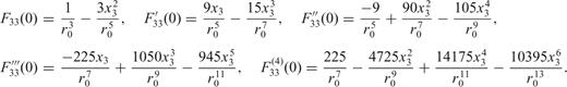
A numerical implementation of eqs (21) and (26) requires using the discrete Fourier transform, or equivalently the Fast Fourier Transform (FFT). This transform operates only on discrete and periodic functions. Let g and h be such functions. The FFT and its inverse are defined as follows (with m₁, p₁, n₁= 0, …, M₁− 1; m₂, p₂, n₂= 0, …, M₂− 1):

29

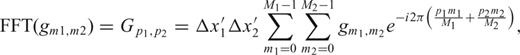
and, the convolution of g and h is defined as

30

The convolution theorem yields:

31

Thus, the numerical equivalent of eq. (21) is

32

and, of eq. (26) it is

33

In eq. (32) it is important to define

34

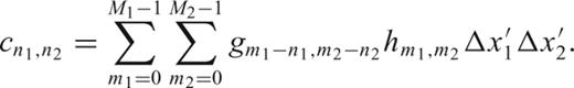
where , such that it is like the result of an FFT applied to a discrete, periodic function. Only this will ensure that the computed gradients are real numbers. That is, in addition to periodicity,

35

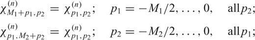
the spectral component, χ⁽ⁿ⁾, must satisfy conjugate symmetry:

36

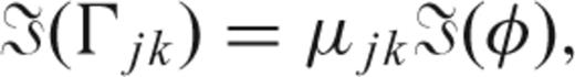
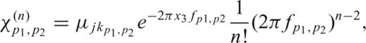
In fact, the quantity, χ⁽ⁿ⁾, defined by eq. (34) with coefficient, μ_jk, given by any of the eqs (19), satisfies the conjugate symmetry property provided that one sets

37

in the case when it is imaginary. Note that χ⁽ⁿ⁾_0,0= 0 in all cases. Thus, χ⁽ⁿ⁾ is obtained for p₁= 0, …, M₁− 1, p₂= 0, …, M₂− 1 by first computing its values according to eq. (34) for p₁=−M₁/2, …, M₁/2 − 1 and p₂=−M₂/2, …, M₂/2 − 1, and then using eqs (35) and (37) (if χ⁽ⁿ⁾ is imaginary). The conjugate symmetry property is satisfied in these cases.

We mention a third type of Fourier transform method that simply applies the convolution theorem to the first of eq. (7), viewed as a 3-D convolution. In this case the density function may be variable in all dimensions and no series expansions are required in the height coordinate (Peng 1995). This method is outside the present scope and requires careful study of potential deleterious effects due to the sharp density contrast at the topographic boundary.

4 Numerical Tests

We compared the terrain-based models for the gravitational gradient using digital elevation data in the western and mid-western U.S. Fig. 3 shows the terrain variation as represented by 1″× 1″ gridded heights. Each area represents a 10′× 10′ spherical patch that is approximated as a plane with grid intervals given, in metres, by Δx′₁= 1″η cos φ_m [m], Δx′₂= 1″η [m], where φ_m is the mean latitude of the patch and η is the arcsec-to-metre conversion factor for a sphere of radius, R= 6371 km. The density of the topographic masses is assigned the constant value, ρ= 2670 kg m⁻³. Without loss in generality, the masses included in the various gradient models are bounded below by the minimum elevation in each area, while the points of evaluation are located at constant height, Δx₃, above the maximum elevation: x= (x₁, x₂, x⁰₃), where x⁰₃=x′_3,max+Δx₃; in our tests, Δx₃= 10 m (see Fig. 4). The evaluation points have horizontal coordinates, (x₁, x₂), identical to the grid points of the terrain elevation data, and lie along a single profile across each test area, as indicated in Fig. 3. The heights of these computation profiles with respect to the underlying topography are shown in Fig. 4, which also shows the gradient, Γ₃₃; the other gradients have roughly similar magnitude.

Figure 3

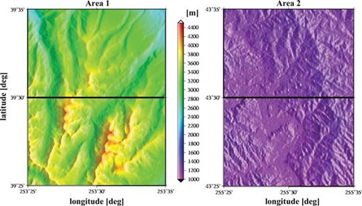
1″× 1″ elevation data in two 10′× 10′ test areas. Left: Area 1 (central Colorado); Right: Area 2 (eastern Wyoming). Computation profiles run through the middle from west to east. The elevation range for Area 1 is 2400 ≤h≤ 4265 m, and for Area 2 it is 1000 ≤h≤ 1315 m.

Open in new tabDownload slide

Figure 4

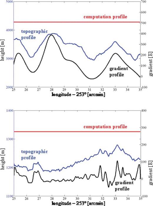
Profiles of topography (left ordinate axis) and Γ₃₃ (right ordinate axis) for Area 1 (top) and Area 2 (bottom). Also shown is the height of the computation profile. The gradient axes are in units of 1 E = 1 Eötvös =10⁻⁹ s⁻².

Open in new tabDownload slide

An internal numerical consistency check of all models is possible for the diagonal (in-line) gradients in the form of Laplace's eq. (Poisson's equation with zero density):

38

Indeed, in all the numerical computations discussed below we found that the maximum value of the left side of this equation was no greater (in absolute value) than 4 × 10⁻⁵ E (1 E = 1 Eötvös = 10⁻⁹ s⁻²), which can be attributed to accumulated computer round-off error.

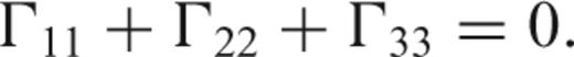
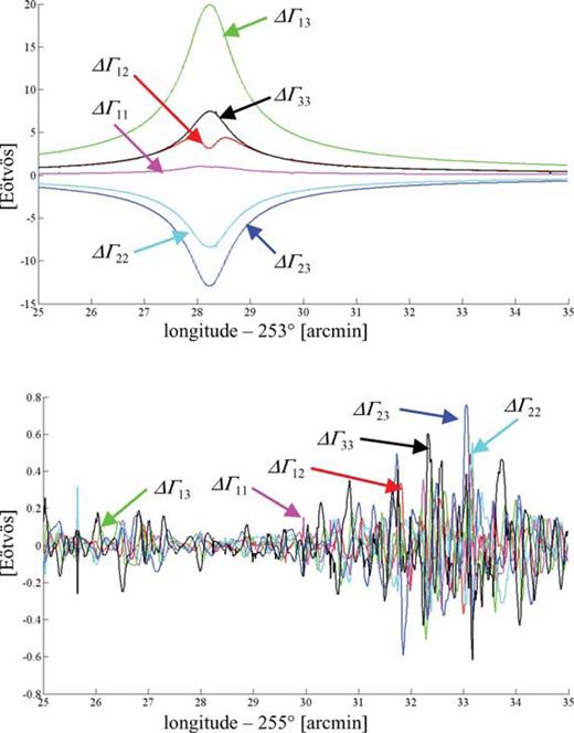
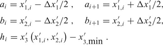
An absolute or external evaluation of the gradient models, on the other hand, requires a truth model that represents the actual gradients due to the topographic masses. At best, such a model can only be conjectured since the terrain elevation data are discrete. For example, one might use the triangulated terrain approximated by piecewise continuous, first-order polynomials (i.e. a polyhedron) to represent the actual topographic surface. Petrovic's formulas (Petrovic 1996; Tsoulis & Petrovic 2001) provide exact corresponding gradients. On the other hand, this‘true’ representation depends on the type of triangulation—for example, since the grid is regular a straightforward (Delauney) triangulation yields grid diagonals that are either in the southeast–northwest direction, or in the southwest–northeast direction, or a combination of these. Fig. 5 shows the differences in the gradients generated by two alternative triangulations, where all diagonals are either in one or the other direction. The noticeably dissimilar character of the differences in these two areas is an artefact of the parameters of the test and the properties of the terrain models. The differences reach 10–20 E for some of the gradients in the rough Area 1 even though the computation points are substantially further from the generating masses than in the smooth Area 2, where the differences are less than 1 E. Fig. 6 hints at the reason for the large discrepancies in Area 1, showing that with all diagonals in the southeast–northwest orientation, the height differences along the diagonals are relatively more uniform than with the alternative orientation. In the smoother Area 2, the distribution of height differences along diagonals is almost independent of their orientation and the gradient differences are likewise close to zero (see Fig. 5). The essential conclusion is that a‘truth’ model eludes our present analysis. Such a model would have to depend uniquely on the data in a manner that best represents the consequent gravitational gradients. Data-dependent triangulation methods may be found in (Dyn 1989), but additional analyses must determine if they optimally represent the gradients.

Figure 5

Differences between gradients generated by triangulated prisms of the DEM using southwest–northeast and southeast–northwest diagonals. Top: profile in Area 1; bottom: profile in Area 2.

Open in new tabDownload slide

Figure 6

Histograms of height differences of diagonal endpoints for southwest–northeast and for southeast–northwest triangulations. The height differences are computed for a 100″× 100″ area centred on the point (28.3 arcmin) of the computation profile in Area 1 (top) and on (28.3 arcmin) in Area 2 (bottom).

Open in new tabDownload slide

Fig. 7 compares the gradients computed according to the right-rectangular prism model against those generated by the triangular prism model using the southeast–northwest diagonal orientation. The right-rectangular prisms are centred on the DEM grid points, so that in eqs (10) and (11),

39

Combining the results of Figs 5 and 7, one finds that in Area 1 the rectangular prism model yields gradients much closer to those generated by the southeast–northwest diagonal triangulation than by the alternative triangulation. This indicates that the former is perhaps a better‘truth’ representation of the topographic surface (for Area 1), if one accepts that the rectangular prisms tend to represent an average of the terrain.

Figure 7

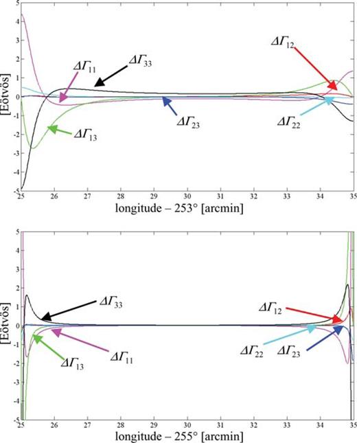
Differences along the computation profile between gradients generated by triangulated prisms (southeast–northwest diagonals) and by rectangular prisms for Area 1 (top) and Area 2 (bottom).

Open in new tabDownload slide

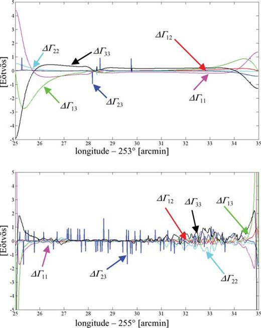
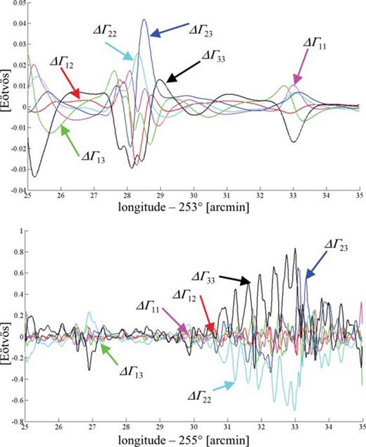
Fig. 8 shows differences between the rectangular numerical integration (eq. 13) and the gradients generated by the rectangular prisms (Areas 1 and 2). The differences in Area 2 are relatively larger because the computation profile is closer to the terrain. Differences between the rectangular and the triangular numerical integrations (eqs 13 and 14) are depicted in Fig. 9 and show that they are significant at the few-Eötvös level only near the edges of the integration areas. It is easy to show that the triangular numerical integration is (almost) independent of the orientation of the diagonals used in the triangulation (only the corner points of the overall rectangular area are weighted differently). Table 1 contains the statistics of the differences shown in Figs 7–9.

Figure 8

Differences along the computation profile between gradients generated by rectangular prisms and by the rectangular numerical integration for Area 1 (top) and Area 2 (bottom).

Open in new tabDownload slide

Figure 9

Differences along the computation profile between gradients computed by the rectangular and triangular numerical integration methods for Area 1 (top) and Area 2 (bottom).

Open in new tabDownload slide

Table 1

Statistics^a for the differences in gradients shown in Figs 7, 8 and 9. All units are Eötvös [E].

Open in new tabDownload slide

The prism methods and the numerical integrations could easily be adapted to generate the gradients at points with arbitrary altitudes above the topographic surface. The FFT models used here, on the other hand, require that all computation points reside at a constant altitude (and on a regular grid) above the entire terrain. The accuracy of these models may be assessed absolutely since in theory (if the series converges) the FFT method is identical to the rectangular numerical integration (provided the circular convolution error is eliminated (Jekeli 1998; Haagmans 1993), as done here). Fig. 10 compares Parker's FFT method, eq. (21), to the rectangular numerical integration model; while Forsberg's FFT method, eq. (26), is assessed similarly in Fig. 11. The critical parameter in these comparisons is the order of expansion of the series. Clearly, there is a direct correlation between the required order of expansion (for comparable accuracy) and the roughness of the terrain.

Figure 10

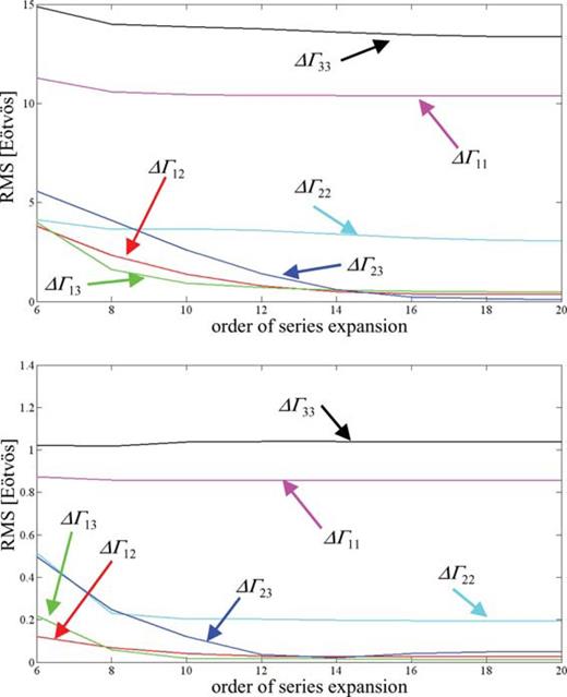
The rms of the differences between gradients computed by rectangular numerical integration and by Parker's FFT method, as a function of the order of the series expansion of the latter, for (top) Area 1 and (bottom) Area 2.

Open in new tabDownload slide

Figure 11

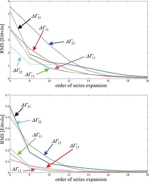
The rms of the differences between gradients computed by rectangular numerical integration and by Forsberg's FFT method, as function of the order of the series expansion of the latter, for (top) Area 1 and (bottom) Area 2.

Open in new tabDownload slide

Forsberg's FFT method converges as required to the rectangular numerical integration method (convergence at the very high orders of expansion may be compromised by computer round-off error). On the other hand, the diagonal (in-line) gradients computed by Parker's FFT method (and to a noticeable extent the off-diagonal gradients) fail to converge to those determined by the numerical integration. This is caused by the continuous, global Fourier transform embedded in the method that ultimately is applied to only discrete and locally extended data.

Finally, we show in Table 2 the computation times required for each type of model. Such comparisons are at best of relative value since they are specific to a computer platform (in this case, dual Intel Itanium 733 MHz processors with 4 Gbyte RAM). Furthermore, the computer code was not necessarily equally efficient for all models, and some adaptive methods could be implemented for the numerical integrations that take advantage of the diminishing contributions of distant zones. Clearly, however, the FFT methods, automatically yielding results for all points on the data grid, are orders of magnitude faster than any of the other methods (if the latter would be used to yield gradients on the entire grid, not just a profile).

Table 2

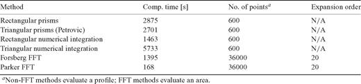
Computation times for various gradient models based on topographic mass sources.

Open in new tabDownload slide

5 Summary

A number of models can be used to represent the gravitational gradients generated by masses that are implied by topographic data. We investigated both finite element (fully analytic integration) methods as well as hybrid analytic/numerical integration of Newtonian potential integrals. The numerical integration can be facilitated by implementing discrete Fourier transforms of the elevation data, if these and the evaluation points are on a regular Cartesian grid. Different formulations have different requirements; most rely on a series expansion of the height.

For two test areas representing rough and moderate topographies, we analysed these methods for computation points along profiles at constant altitude (above all the terrain). We found only small differences in the gradients between rectangular and triangular numerical integration (≤0.33 E (rms) along the profile in Area 1; ≤0.05 E (rms) along the profile in Area 2; see Fig. 9). Triangulated finite element representations of the topographic masses, however, can generate significantly different gradients depending on the triangulation of the domain points (see Fig. 5). On the other hand, very small differences were found between the rectangular prism and the rectangular numerical integration methods (≤0.01 E (rms) along the profile in Area 1; ≤0.23 E (rms) along the closer profile in Area 2; see Fig. 8).

The FFT techniques ostensibly are faster, despite the many convolutions that are evaluated in the series expansion with respect to topographic heights. Two types of expansion were tested and the one by Parker (1972) was found to yield unacceptable biases (see Fig. 10) in the computed in-line gradients (compared to the rectangular integration method that it approximates). Both Tziavos (1988) and Schwarz (1990) also used the Parker FFT expansion, but were unaware of such biases since they made no comparison to the more rigorous rectangular numerical integration (or rectangular finite element method). For evaluation points close to rough terrain, quite high orders of expansion are required (14, in our case) to achieve sub-Eötvös accuracy with the alternative FFT method by Forsberg (1985); see Fig. 11.

Acknowledgments

This work was sponsored by the National Geospatial-Intelligence Agency under contract NMA401-02-1-2005. The authors are indebted to anonymous reviewers for helping to improve the manuscript.

References