


Summary
The Galápagos volcanic province (GVP) includes several aseismic ridges resulting from the interaction between the Galápagos hotspot (GHS) and the Cocos–Nazca spreading centre (CNSC). The most prominent are the Cocos, Carnegie and Malpelo ridges. In this work, we investigate the seismic structure of the Carnegie ridge along two profiles acquired during the South American Lithospheric Transects Across Volcanic Ridges (SALIERI) 2001 experiment. Maximum crustal thickness is ∼19 km in the central Carnegie profile, located at ∼85°W over a 19–20 Myr old oceanic crust, and only ∼13 km in the eastern Carnegie profile, located at ∼82°W over a 11–12 Myr old oceanic crust. The crustal velocity models are subsequently compared with those obtained in a previous work along three other profiles over the Cocos and Malpelo ridges, two of which are located at the conjugate positions of the Carnegie ones. Oceanic layer 2 thickness is quite uniform along the five profiles regardless of the total crustal thickness variations, hence crustal thickening is mainly accommodated by layer 3. Lower crustal velocities are systematically lower where the crust is thicker, thus contrary to what would be expected from melting of a hotter than normal mantle. The velocity-derived crustal density models account for the gravity and depth anomalies considering uniform and normal mantle densities (3300 kg m−3), which confirms that velocity models are consistent with gravity and topography data, and indicates that the ridges are isostatically compensated at the base of the crust. Finally, a two-dimensional (2-D) steady-state mantle melting model is developed and used to illustrate that the crust of the ridges does not seem to be the product of anomalous mantle temperatures, even if hydrous melting coupled with vigorous subsolidus upwelling is considered in the model. In contrast, we show that upwelling of a normal temperature but fertile mantle source that may result from recycling of oceanic crust prior to melting, accounts more easily for the estimated seismic structure as well as for isotopic, trace element and major element patterns of the GVP basalts.
1 Introduction
The origin of large igneous provinces and aseismic ridges is usually associated with the presence of hot mantle plumes rising from the deep mantle, whose surface imprint is referred to as hotspot (Wilson 1963; Morgan 1971). The thermal plume model asserts that a hot, rising plume enhances mantle melting and that the excess of melting is mostly emplaced as igneous crust (McKenzie & Bickle 1988; White & McKenzie 1989, 1995). The primary support for this hypothesis is the thick crust of both aseismic ridges and igneous provinces as compared with normal oceanic crust (e.g. Coffin & Eldholm 1994; Charvis et al. 1995; Darbyshire et al. 2000; Charvis & Operto 1999; Grevemeyer et al. 2001; Sallarès et al. 2003). The crustal overthickening is reflected in the prominent topography and gravity anomalies that characterize these structures (Anderson et al. 1973; Cochran & Talwani 1977). Additional arguments repeatedly invoked to support the thermal plume model include:
- (i)
the composition of the hotspot basalts, which generally exhibit a distinct geochemical signature from the mid-ocean ridge basalts (MORB) and is in agreement with that expected for melting of a hotter than normal mantle (Watson & McKenzie 1991; White et al. 1992);
- (ii)
the high-velocity crustal roots frequently found in oceanic plateaus, aseismic ridges and passive volcanic margins (e.g. Coffin & Eldholm 1994; Kelemen & Holbrook 1995; Grevemeyer et al. 2001); and
- (iii)
the mantle low-velocity anomalies extending from the surface to the lower mantle shown by global tomography models, particularly in Iceland (Bijwaard & Spakman 1999; Ritsema & Allen 2003).
Regardless of the wide acceptance of the thermal plume model, several alternatives have been also proposed. The small-scale convection model shows that systems cooled from above having lateral temperature contrasts will develop small-scale convection up to an order of magnitude faster than plate motions (e.g. Korenaga & Jordan 2002). In addition, it has been demonstrated that rifting may induce dynamic convection within the mantle as well (Boutilier & Keen 1999). The rapid vertical convection will increase melt production in the upper mantle without the necessity of having hot mantle plumes. It has also been proposed that mantle plumes may include a significant proportion of lower melting components, such as eclogite derived from recycled oceanic crust (Cordery et al. 1997; Campbell 1998). The importance of major element source heterogeneity to account for the excess of melting has been also proposed for a number of hotspots including Hawaii (Hauri 1996), Açores (Schilling et al. 1983) and Iceland (Korenaga & Kelemen 2000). It has been also suggested that some so-called hotspots are actually wet-spots of normal temperature (e.g. Açores), based on the composition of the abyssal peridotites (Bonatti 1990). Last but not least, recent seismic experiments show that high-velocity crustal roots are absent in the Greenland margin (North Atlantic volcanic province) (Korenaga et al. 2000), and the Cocos and Malpelo ridges (Galápagos volcanic province, GVP; Sallarès et al. 2003), and none of the local tomography studies yet performed in Iceland shows compelling evidence of a velocity anomaly extending deeper than the mantle transition zone (e.g. Foulger et al. 2001; Wolfe et al. 2002).
The GVP constitutes a well-studied example of an igneous province generated by the interaction between the Galápagos hotspot (GHS) and the Cocos–Nazca spreading centre (CNSC). Different geophysical studies based mainly on gravity analysis, seismic data and numerical models along the present and palaeo-axes of the CNSC suggest that the GHS is a thermal anomaly (Schilling 1991; Ito & Lin 1995; Ito et al. 1997; Canales et al. 2002), and the receiver function analysis claims that the associated mantle plume extends deeper than the mantle transition zone (Hooft et al. 2003). However, recent seismic modelling along three wide-angle profiles acquired during the Panama basin and Galápagos plume-New Investigations of Intra plate magmatism (PAGANINI-1999) experiment have shown that the velocity and density structure of Cocos and Malpelo aseismic ridges (Fig. 1) is not consistent with that expected for a crust generated by decompression melting of a hot mantle plume (Sallarès et al. 2003). In addition, available global tomography models do not show any Galápagos-linked anomaly going deeper than the base of the upper mantle (Courtillot et al. 2003; Ritsema & Allen 2003; Montelli et al. 2004). In this paper, we present additional velocity models from two new transects acquired across the Carnegie ridge during the South American Lithospheric Transects Across Volcanic Ridges (SALIERI) seismic experiment in 2001 (Flueh et al. 2001; Fig. 1). The velocity models are compared with those previously obtained in Cocos and Malpelo ridges. Then, the velocity-derived density models are used to determine the mantle density structure that best fits the gravity and topography anomalies. Finally, a two-dimensional (2-D) steady-state mantle melting model is developed and used to estimate the range of mantle melting parameters (potential temperature, deep upwelling ratio, presence of a hydrous root) that best explains the crustal structure of the aseismic ridges and thus to infer a possible nature for the GHS.
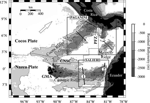
Location map of the study zone showing the residual bathymetry derived from the seafloor age (Mueller et al. 1996), based on the plate cooling model of Parsons & Sclater (1977) for ages smaller than 70 Myr (d= 2500 + 350t1/2). Numbers show crustal ages of oceanic plates at 5 Ma intervals. Large arrows display plate motions relative to the stable South American craton (Trenkamp et al. 2002). Black lines show the location of all the wide-angle seismic profiles and numbers indicate the two profiles used in this work (profile 1, Western Carnegie; profile 2, Eastern Carnegie). Boxes outline the seismic experiments recently performed in Cocos, Malpelo and Carnegie (PAGANINI-1999; SALIERI-2001). CNSC, Cocos–Nazca Spreading Centre; GHS, Galápagos hotspot; PFZ, Panama fracture zone.
2 Tectonic Setting and Previous Work
The GVP is an excellent natural laboratory to investigate melting processes resulting from the interaction between a spreading centre and a melt anomaly. It constitutes several aseismic ridges, which have resulted from the interaction between the CNSC and the GHS during the last 20 Myr The most prominent are the Cocos, Carnegie and Malpelo ridges, which show the imprint of the GHS into the Cocos and Nazca plates (Fig. 1). Different works based on magnetic and bathymetric data suggest that seafloor spreading along the CNSC originated at ∼23 Ma, following a major plate reorganization, which broke the ancient Farallon Plate along a pre-existing fracture zone (e.g. Hey 1977; Lonsdale & Klitgord 1978; Barckhausen et al. 2001). At that time, the GHS was located near the CNSC, and had begun accreting both the Cocos and Carnegie ridges.
At present day, the GHS is located beneath the Galápagos archipelago, at ∼190 km south from the CNSC (Fig. 1). Recent Global Positioning System (GPS) measurements indicate that the Nazca Plate is moving approximately towards 90°NE at 58 ± 2 km Myr−1 and the Cocos Plate towards 41°NE at 83 ± 3 km Myr−1 with respect to the stable South American craton (Freymueller et al. 1993; Trenkamp et al. 2002). Those motions are basically the addition of ∼60 km Myr−1 seafloor spreading along the CNSC (Sallarès & Charvis 2003), E–W spreading along the East Pacific Rise (∼110 km Myr−1 at 2°N, based on DeMets et al. 1990) and ∼26 km Myr−1 northward migration of the CNSC in the GHS reference frame (Sallarès & Charvis 2003). The CNSC migration, together with the occurrence of ridge jumps along the spreading axis between 19.5 and 14.5 Ma, have resulted in significant variations in the relative location of the GHS and the CNSC during the last 20 Myr. Between 20 and ∼12 Ma, the GHS was approximately ridge-centred, between ∼12 and 7.5 Ma it was located beneath the Cocos Plate, and from then to now it has been located beneath the Nazca Plate (Barckhausen et al. 2001; Sallarès & Charvis 2003). The Panama fracture zone (PFZ), which is a major tectonic feature of the GVP, opened at ∼9 Ma, triggered by the cessation of the easternmost Cocos Plate subduction beneath Middle America. The strike-slip motion along the dextral PFZ lead to the separation between the Cocos and Malpelo ridges (Sallarès & Charvis 2003).
A large number of geophysical and geochemical studies have been performed in the GVP. These works include:
- (i)
geochemical analysis and dating of samples dredged along the present-day ridge axis and across the aseismic ridges (Schilling et al. 1982; Verma et al. 1983; Hoernle et al. 2000; Detrick et al. 2002);
- (ii)
gravity and topography analysis along the present and palaeo-axes of the CNSC (Schilling 1991; Ito & Lin 1995; Canales et al. 2002);
- (iii)
numerical modelling of the plume–ridge interaction (Ito et al. 1996, 1999);
- (iii)
identification and reconstruction of magnetic anomalies (Hey 1977; Lonsdale & Klitgord 1978; Hardy 1991; Wilson & Hey 1995; Barckhausen et al. 2001);
- (iv)
receiver function analysis at the Galápagos platform (Hooft et al. 2003); and
- (v)
wide-angle seismic models of the crustal structure across the Cocos and Malpelo ridges (Trummer et al. 2002; Walther 2002; Sallarès et al. 2003; Walther 2003), the Galápagos platform (Toomey et al. 2001) and the CNSC (Canales et al. 2002).
The results of these studies have been also used to infer the geodynamic evolution of the GVP (e.g. Hey 1977; Barckhausen et al. 2001; Sallarès & Charvis 2003) and to estimate the excess temperature associated with the presence of the GHS along the present ridge and palaeoridge axis of the CNSC (Schilling 1991; Ito & Lin 1995; Canales et al. 2002). A quantitative estimation of the influence of the distinct melting parameters on the crustal structure observed at the Cocos, Carnegie and Malpelo ridges, however, has been so far lacking.
3 Wide-Angle Data Set
The seismic data set used in this study constitutes 52 seismic sections recorded along two wide-angle profiles, which were acquired in the summer of 2001 during the SALIERI cruise aboard the German R/V Sonne. Shooting along both profiles was conducted using three 2000 cubic inch airguns and a firing interval of 60 s, with a shot spacing of around 120 m. The set of receivers constituted 24 Geomar ocean bottom hydrophones (OBH) and ocean bottom seismometers (OBS) together with 13 Institut de Recherche pour le Développement (IRD) OBS. The first profile (profile 1 in Fig. 1) includes 30 OBS and OBH that were deployed along a 350 km N–S trending transect, which crosses the saddle of the Carnegie ridge at ∼85°W. The receiver spacing along this line was between 7 and 15 km. The second profile (profile 2 in Fig. 1), comprises 22 instruments deployed along a N–S transect of 230 km covering the northern flank of the ridge near the subduction zone, at ∼82°W. Receiver spacing was similar to that of profile 1. The location of both seismic lines and those of three other transects acquired across the Cocos and Malpelo ridges during the PAGANINI-1999 experiment are shown in Fig. 1.
The data acquired along both profiles have a very good quality. Systematic data processing consisting of time and distance depending predictive deconvolution and frequency filtering, and automatic gain control was applied to the recorded seismic gathers (see parameters in Table 1). Several of the record sections are shown in Fig. 2. The seismic phases observed in all record sections are predominantly first arrivals corresponding to waves refracted within the oceanic crust (Pg) and clear secondary arrivals identified as reflections in the crust–mantle boundary (PmP). In a few record sections from instruments located at the northern flank of the Carnegie ridge deeper phases corresponding to the refraction within the uppermost mantle (Pn) can also be observed (e.g. Fig. 2a and f). Interestingly, PmP is not observed in these record sections, thus we included the Pn phases to have an estimate of the crustal thickness in the northern flank of the ridge. The seismic phases can be easily followed up to more than 150 km from the source in most record sections (e.g. Fig. 2f). The reciprocity of traveltimes was checked out to verify the consistency of picked phases between different instruments.
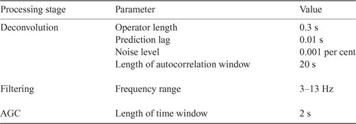
Values of the different parameters used in the seismic data processing.
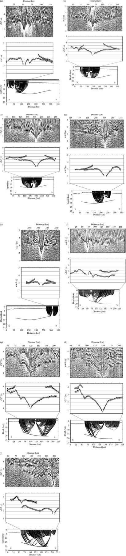
Seismic gathers recorded along the numbered profiles of Fig. 1. Systematic data processing consisting of 5–15 Hz butterworth filtering, predictive deconvolution and automatic gain correction was applied to all the gathers (top). Picked traveltimes (solid circles with error bars) and predicted traveltimes (open circles) for Pg and PmP phases using the velocity models displayed in Fig. 3 (middle). Ray tracing corresponding to the same models (bottom). (a) Ocean bottom seismometers (OBS) 3, profile 1; (b) OBS 10, profile 1; (c) OBS 17, profile 1; (d) OBS 23, profile 1; (e) OBS 29, profile 1; (f) OBS 5, profile 2; (g) OBS 10, profile 2; (h) OBS 13, profile 2; (i) OBS 19, profile 2.
The amplitude of the arrivals and the apparent velocities of the different phases identified in the record sections are very similar to those obtained in the data acquired across the Cocos and Malpelo ridge profiles during the PAGANINI-1999 experiment, which used the same sources and receivers (Sallarès et al. 2003). The refracted phase within the igneous crust (Pg) is observed as a strong arrival in all record sections and its pattern is similar in most of the instruments. At near offsets, it shows low apparent velocities (4–6 km s−1), increasing quickly with distance to around 6.5 km s−1 at 20–30 km from the source, depending on the location of the instrument (Fig. 2). This segment of the phase is probably a refraction within the sediments and the basaltic upper igneous crust (oceanic layers 1 and 2), in which the vertical velocity gradient is likely to be strong as a result of the variations in rock porosity and alteration with depth (e.g. Detrick et al. 1994). Beyond this distance the apparent velocity of the Pg phase is more uniform, exceeding rarely 7.0 km s−1. This flat segment of the phase is interpreted to be a refraction in the upper part of the lower igneous crust (oceanic layer 3), which is mostly composed of gabbros and is less porous and altered than layer 2.
The other phase observed in most record sections is the Moho reflection (PmP). It is observed as a high-amplitude arrival, especially at the thickest crustal segments beneath the crest of the ridge. The main difference between the two profiles is the distance at which PmP becomes indistinguishable from Pg, which provides a qualitative estimation of the differences in crustal thickness along the two profiles. In profile 1, the distance is less than 80 km (Figs 2b and c), while in profile 2 it is as long as 150 km (Figs 2f and i), indicating that the crust is considerably thicker along profile 2. In the deep ocean basin located south of the Carnegie ridge, PmP is observed at near-offsets (∼20 km), and PmP and Pg become indistinguishable at approximately 30–40 km from the source (Fig. 2e). This is consistent with a reflection from the Moho of a fairly normal oceanic crust (7–8 km).
Picking of Pg and PmP phases was done manually. Picking errors were assigned to be half a period of one arrival, to account for a possible systematic shift in the identification of the arrivals. In addition, they were overweighted or downweighted depending on the quality of the phase. For Pg phases, errors are around 40–50 ms for near offsets and 50–60 ms for far offsets. For PmP phases, they are ∼80 ms on average.
4 Seismic Tomography
2-D velocity models along both profiles were estimated using the joint refraction and reflection traveltime inversion method of Korenaga et al. (2000). This method allows the determination of a 2-D velocity field together with the geometry of a floating reflector from the simultaneous inversion of first arrivals and secondary reflections traveltimes. The uncertainty of the obtained model parameters is estimated by performing a Monte Carlo–type analysis, which is identical to that described in Sallarès et al. (2003). The main steps of the inversion procedure are as follows: (i) A one-dimensional (1-D) averaged velocity model and a Moho depth are calculated. This model is used as a reference model to perform the inversion. (ii) A set of 100 1-D initial models is constructed by randomly perturbing the Moho depth (±3 km) and the velocity of the crustal nodes (±0.3 km s−1) of the 1-D reference model. Besides, 100 noisy data sets are built by adding random picking errors (±25 ms) to each arrival from the initial data set, together with common phase errors accounting for a possible systematic shift in the picking of a given seismic phase (±50 ms) and common receiver errors (±50 ms). (iii) The 2-D model is parametrized and a 2-D inversion is performed for each random initial model with a random data set.
Our preferred final solution along both profiles is the average of all the Monte Carlo realizations (Fig. 3). The standard deviation of velocity and depth parameters with respect to the final solution can be considered as a statistical measure of the uncertainties (Tarantola 1987; Matarese 1993). The trade-off between velocity and depth parameters has been tested by performing the inversion with different values of the depth-kernel weighting parameter, w (Korenaga et al. 2000). The internal consistency of the data set and the robustness of the obtained solution have been checked out by comparing the results of two inversions using only one half of the data in each. We also performed checkerboard tests with synthetic data to estimate the resolving power of the data set. For a more detailed description of the inversion procedure and parameters, see Sallarès et al. (2003).
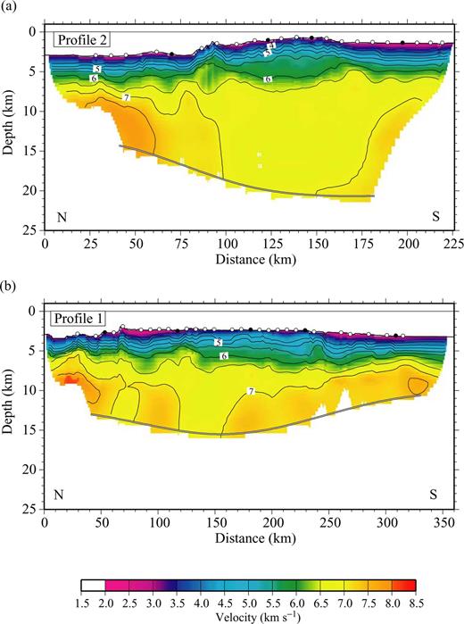
Seismic tomography results. Final averaged velocity models from the 100 Monte Carlo ensembles. (a) Profile 2, eastern Carnegie; (b) profile 1, western Carnegie. Open circles indicate ocean bottom seismometers (OBS)/ocean bottom hydrophones (OBH) locations. Solid circles show the instruments corresponding to the seismic gathers displayed in Fig. 2.
4.1 Results
4.1.1 Inversion parameters
The data set of profile 1 is composed of 6667 Pg and 3682 PmP picked from 30 record sections. The model is 360 km wide and 25 km deep. Horizontal grid spacing is 0.75 km and vertical grid spacing varies from 0.2 km at the seafloor to 1.5 km at the bottom of the model. Spacing of depth parameters is 1.5 km. We use horizontal correlation lengths varying from 8 km at the top of the model to 16 km at the bottom and vertical correlation lengths ranging from 0.2 km at the top to 3 km at the bottom for the velocity inversion. Variations of up to 50 per cent of these parameters lead to very similar results in terms of smoothness of the inverted velocity models. We tried three different values of w= 0.1, w= 1 and w= 10 for the depth weighting parameter. The rms traveltime misfit for the 1-D average model is 272 ms (χ2∼ 15) and for the average model of all the 100 Monte Carlo realizations (with w= 1) it is 69 ms (χ2∼ 1.1). In profile 2, the data set is composed of 5889 first arrivals and 2147 PmP from 22 OBS and OBH. The model is 230 km wide and 25 km deep, grid spacing is 0.5 km horizontally, and it varies between 0.2 and 1.5 km vertically. Depth parameters are 1.5 km spaced. Horizontal and vertical correlation lengths are the same as those described for profile 1. Rms for the 1-D average model is 390 ms (χ2∼ 15) and for the final model (w= 1) is 71 ms (χ2∼ 1.2). The average velocity models of all the Monte Carlo realizations corresponding to both profiles are shown in Fig. 3. The fit between observed and calculated traveltimes and the ray tracing across the models for several instruments are shown together with the record sections in Fig. 2.
4.1.2 Seismic structure
The velocity structure is very similar along both profiles, and also analogous to that previously obtained at Cocos and Malpelo (Sallarès et al. 2003). The crust is divided into two layers, which can be identified with oceanic layers 2 (and the sediment cap) and 3. Layer 2 shows a notable vertical velocity gradient, with velocities varying from approximately 3.0 to 6.5 km s−1. The isovelocity contour of 6.5 km s−1 corresponds to a major change in velocity–depth gradient that we attribute to the boundary between layers 2 and 3 (Fig. 3). In layer 3, velocity is much more uniform, and ranges between ∼6.8 and ∼7.2 km s−1. Similarly to Cocos and Malpelo, the lowest layer 3 velocities are generally found where the crust is the thickest (i.e. beneath the crest of the ridge), although mean layer 3 velocities are not necessarily the same for a given crustal thickness in the different profiles. The maximum crustal thickness estimated along profile 1, located over 11–12 Myr old seafloor, is around 13 km, while along profile 2 (∼20 Myr old seafloor) it is ∼19 km (Fig. 3). Maximum crustal thickness estimated along their conjugated profiles acquired during the PAGANINI-1999 experiment (Fig. 1) are ∼16.5 km (12 Ma) and ∼19 km (20 Ma), respectively (Sallarès et al. 2003). The velocity structure obtained across the Carnegie ridge profiles is very similar to that obtained in another profile located south of the bulge of the Carnegie ridge, perpendicular to the trench axis, which extends from the outer rise to the coastline (Graindorge et al. 2003). This velocity model shows a crustal thickness of ∼14 km, with almost all the crustal overthickening accommodated in a 7.0–7.2 km s−1 crustal root that corresponds to the oceanic layer 3.
The similarity of the velocity structure across the different transects indicates that the process of formation of all the ridges (i.e. the nature of the GHS) is likely to be the same. Moreover, the crustal thickness variations reveal that the relative intensity of the GHS at both sides of the CNSC has changed with time, indicating the existence of significant variations in the relative distance between these two structures (Sallarès & Charvis 2003). The thickness of layer 2 is quite uniform (3.5 ± 1.0 km) regardless of the total crustal thickness variations. This means that the crustal thickening of the aseismic ridges is mainly accommodated by layer 3, in agreement with what is observed in most overthickened oceanic crustal sections (e.g. Mutter & Mutter 1993). The only exception to this general tendency is the northern flank of the Carnegie ridge, where layer 2 (and the whole crust) is significantly thinner than in the other parts of the transects. Here, the Moho geometry is not controlled by PmP, but the presence of a conspicuous shallow (<8 km depth) and high-velocity (∼7.5–8.0 km s−1) mantle-like anomaly indicates that the oceanic crust must be only 6–7 km thick (Fig. 3). Therefore, the Moho geometry could be highly asymmetric, showing a steeper transition between the crest of the ridge and the adjacent oceanic basin in the northern flank of the ridge (i.e. that which is closest to the CNSC) than in the southern flank. A similar type of behaviour was also observed in the conjugated segment of profile 1 over the Cocos ridge, where a steeper transition is observed in the inner, SE flank of the ridge, than in the outer, NW flank (Sallarès et al. 2003).
4.1.3 Uncertainty analysis
The statistical uncertainties of model parameters obtained by averaging the solutions of all 100 Monte Carlo realizations for both profiles are shown in Figs 4(a) and (c). The derivative weight sum (DWS), which is the column-sum vector of the Fréchet partial derivatives matrix (Toomey & Foulger 1989), is shown in Figs 4(b) and (d). Velocity uncertainty is lower than 0.1 km s−1 within most parts of the models. Layer 2 velocities show generally the lowest uncertainties (<0.05 km s−1). However, uncertainties are slightly higher in the upper half of this layer, where velocity gradient is larger, than in the bottom half. Uncertainties in layer 3 are generally smaller than 0.1 km s−1, with several local anomalies where uncertainty is somewhat larger (∼0.15–0.20 km s−1). Depth uncertainties are lower than 0.3–0.4 km along most of the section. The largest velocity (>0.2 km s−1) uncertainties are obtained in the layer 3 of the northern segment of profile 2 (near 50 km model distance). Consistently, PmP phases are not observed in this part of the transect. In layer 2, velocity can be well determined from Pg traveltimes. In contrast, Pg phases rarely go through the lower part of layer 3 (Figs 4b and d), so both the lower crustal velocity and Moho geometry information are contained uniquely in PmP traveltimes. Because inversions with reflection traveltimes are subject to velocity–depth ambiguities, the Moho depth and lowermost crust velocity uncertainties tend to be correlated, as can be observed in Fig. 2(a).
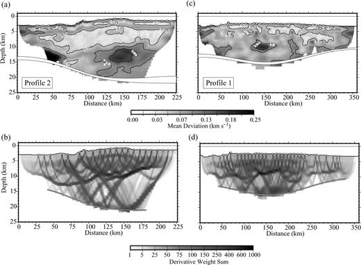
Velocity and Moho depth uncertainties corresponding to the average of the 100 Monte Carlo realizations (top) and derivative weight sum (DWS; bottom) obtained with the velocity models displayed in Fig. 3. (a, b) Profile 2, eastern Carnegie; (c, d) profile 1, western Carnegie.
4.1.4 Resolution and accuracy
A classical manner to estimate the resolving power of a given data set with a particular experiment layout is to perform checkerboard tests. We have built a reference model by adding sinusoidal anomalies with a maximum relative amplitude of 5 per cent to our preferred solution in the upper crust (13 × 6 km) and lower crust (35 × 12 km). The reference model and the inverted solution for both profiles are shown in Fig. 5. The inversion with synthetic data was performed using as an initial model a 1-D crustal velocity model with a flat Moho, corresponding to the best fit of all traveltimes. The data set constitutes the traveltimes calculated with the reference model, to which we added picking, common phase and common shot errors (see description in Section 4). The pattern of the velocity anomalies is well recovered at both upper and lower crustal levels. In general, we can conclude that teometry of the experiment is appropriate and thus the data set is sensitive enough to resolve velocity anomalies of the size considered here, with lateral velocity contrasts lower than 0.2 km s−1 in the upper crust and lower than 0.3 km s−1 in the lower crust. Moreover, the Moho geometry is well recovered along most of the model with differences lower than 0.4 km, in agreement with the results of the uncertainty analysis. However, checkerboard tests are an incomplete demonstration of the degree of the ambiguities, because they are always limited to very specific velocity models with particular anomalies. Instead, Korenaga et al. (2000) proposed a practical way to do that by systematically exploring the result of the inversion using different values for the depth-kernel weighting parameter, w, which controls the relative weighting of velocity and depth parameters in reflection tomography. We did the test using w= 0.1 and w= 10. The results are very similar to those obtained with w= 1, showing always the overall anticorrelation between crustal thickness and layer 3 velocity, which indicates that velocity–depth trade-off is not important and it does not alter the main results of the work. Finally, we performed a last test to evaluate the consistency of the results in profile 1, which consisted of repeating the inversion twice with the 1-D average model as an initial model but using only the data from one half of the instruments on each inversion. The results are shown in Fig. 6. The long-wavelength structure obtained using both data sets is very similar, showing the same crustal thickness and similar features along the whole profile. Differences are local and small. The remarkable resemblance of the solutions obtained using two totally independent data subsets confirms the internal consistency of the whole data set, and demonstrates that most velocity anomalies are real features and that inversion artefacts, if present, are minor.
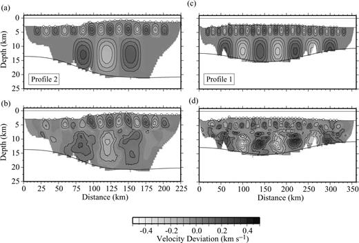
Results of the checkerboard tests. Synthetic models showing the amplitude of velocity anomalies with respect to the background models displayed in Fig. 3 (top) and results of tomographic inversion (bottom). (a, b) Profile 2, eastern Carnegie; (c, d) profile 1, western Carnegie.
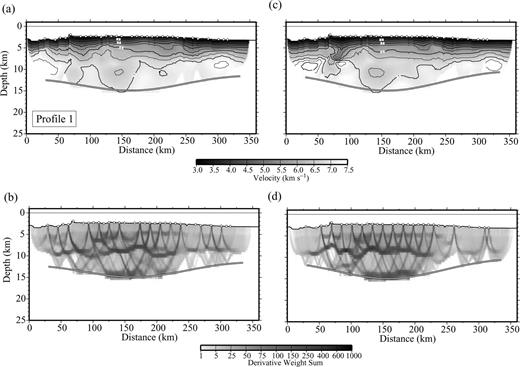
Results of two inversions using only one half of the instruments on each. Velocity models (top) and derivative weight sum (DWS; bottom) obtained using 15 Geomar ocean bottom hydrophones (OBH; a, b), and with 13 Institut de Recherche pour le Développement (IRD) ocean bottom seismometers (OBS) and 2 Geomar OBH (c, d).
5 Gravity and Compensation Of Topography
Large igneous provinces and aseismic ridges typically show broad swells, which are characterized by striking topography and gravity anomalies (Schilling 1985; Sleep 1990). Swells are believed to be supported by a combination of crustal thickening and sublithospheric mantle density anomalies of thermal and/or chemical origin (Oxburgh & Parmentier 1977; Courtney & White 1986; Phipps Morgan et al. 1995), but the relative importance of each factor to support the swell is a matter of discussion. One end-member is the mantle plume model, which affirms that the primary sources of plume buoyancy are mantle thermal anomalies (White & McKenzie 1989, 1995). Another alternative is a combination of hotter than normal mantle temperatures and mantle density variations arising from melt depletion (Phipps Morgan et al. 1995). In both cases, the mantle column beneath hotspot swells would have to show anomalous seismic velocities and densities related with the presence of the mantle plume. The contribution of the mantle anomalies is likely to be significant for oceanic swells located above active hotspots or melting anomalies, as indicated by seismic and gravity data in Iceland (Wolfe et al. 1996; Darbyshire et al. 2000), Hawaii (Laske et al. 1999) and the present-day GHS-influenced area (Canales et al. 2002; Hooft et al. 2003).
The other end-member is the crustal compensation model, in which the swell is largely compensated by lateral variations of crustal density and Moho topography, with a minor contribution of mantle density anomalies. This seems to be the case, for instance, of the Marquesas swell, where buoyancy of the material underplating the island chain has been shown to be able to support almost completely the swell (McNutt & Bonneville 2000). These authors suggested that this can be also the case for other swells, such as Hawaii or the Canary Islands. In this case, the upper-mantle velocity and density anomalies are likely to be small, perhaps undetectable for seismic methods. The crustal compensation may be a plausible model to account for oceanic swells located away from the zone of direct influence of the mantle plume. This is apparently the case of the Cocos and Malpelo ridges, in the GVP (Sallarès et al. 2003), although a previous gravity analysis of the GVP suggests that mantle density anomalies associated with the presence of the GHS are still significant ∼8 Myr after the emplacement of the ridge and ∼400 km away from the hotspot location (Ito & Lin 1995). Between the two end-member cases, there are a number of different possibilities. Canales et al. (2002), for example, argued that the Galápagos swell is sustained by a combination of crustal thickening (∼50 per cent), thermal buoyancy (∼30 per cent) and chemical buoyancy arising from melt depletion (∼20 per cent).
In this section, we show the results of a gravity analysis along profile 1 (Fig. 1). We chose this profile because it is located mid-plate, far away from the margin, and the assumption of lateral homogeneity is valid in this case. Our purpose is to calculate the velocity-derived crustal density structure, and to estimate then the range of mantle density anomalies required to explain the observed gravity and topography data along the profile. Velocity-derived density models across Malpelo and Cocos are also available in Sallarès et al. (2003). The similarity of the crutal structure between this profile and the other profiles acquired in Carnegie, Cocos and Malpelo, makes it possible to extrapolate the results obtained to the other ridges of the GVP.
5.1 Density models and gravity analysis
The gravity profile along the transect has been built using available marine gravity data based on satellite altimetry (Sandwell & Smith 1997). We have employed a code based on the Parker (1972) spectral method to calculate the gravity anomaly produced by a heterogeneous 2-D density model. We first calculated the gravity anomaly generated by a single crustal layer with the crust–mantle boundary geometry from the velocity model and uniform density (2800 kg m−3). This model fits the observed anomaly with a misfit of ∼30 mGal, but it underestimates the anomaly at the centre of the ridge and at the northern flank, where the Moho geometry derived from seismic tomography is worst resolved. In the second model, the velocity model from Fig. 3(a) was directly transformed to densities using different empirical conversion laws for the different crustal layers. For velocities lower than 3.2 km s−1 (which we considered to be sediments), we have applied the velocity–density relationship of Hamilton (1978) for shale, ρ= 0.917 + 0.747Vp− 0.08Vp2, while for higher velocities we have assumed Carlson & Herrick's (1990) empirical relation for oceanic crust, ρ= 3.61 − 6.0/Vp, which is based on Deep Sea Drilling Project (DSDP) and Ocean Drilling Program (ODP) core data. Mantle density has been fixed to 3300 kg m−3. Following the procedure described in Sallarès et al. (2003), we have calculated the densities from seismic velocities at in situ conditions using the estimates of the pressure and temperature partial derivatives (e.g. Korenaga et al. 2001). Because the Moho geometry of the northern flank of the ridge (0–75 km along profile) is poorly constrained by the seismic data, we have varied the Moho depth in this part of the transect until a good match of the gravity data has been obtained.
The estimated density model (Fig. 7a), shows a highly asymmetric Moho geometry. The transition between the top of the bulge and the adjacent oceanic basin is more abrupt in the northern flank of the ridge than in the southern flank. In the north, the oceanic basin is ∼6 km thick, while in the south the crust is ∼8 km thick. The velocity-derived density model explains the observed gravity anomaly with a misfit of less than 6 mGal, indicating that the velocity model is compatible with the gravity data within the model uncertainty without the necessity of considering mantle density anomalies (Fig. 7b). The results are thus consistent with those previously obtained in the Cocos and Malpelo ridge profiles (Sallarès et al. 2003).
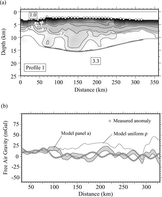
(a) Velocity-derived density model along profile 1, western Carnegie. Densities are in g cm−3. (b) Observed free-air gravity anomaly (open circles) and calculated gravity anomaly for model displayed in panel (a). Shaded zone shows the gravity anomaly uncertainty inferred from the Monte Carlo analysis. The rms misfit for this model is 6 mGal. Dashed line corresponds to the constant density model (2800 kg m−3) with the Moho obtained from the tomographic inversion.
5.2 Isostasy model
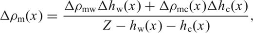

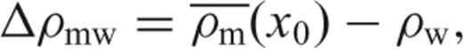


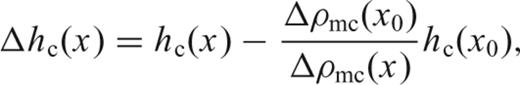
 and
and  are the averaged crustal and mantle densities, hw(x) is the water depth and hc(x) is the crustal thickness, of a lithospheric column located at x. The definition and value of all constants and variables used in the model is given in Table 2.
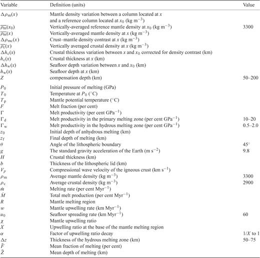
Definition, units and values of all the constants and variables used throughout the calculations.
The only unknown in eq. (1) is thus Z, the compensation depth above which we assume that all lateral density anomalies are confined. We have estimated the mantle density variations required, Δρm(x), to fit the observed bathymetry along the density models estimated at profile 1 in Carnegie (Fig. 7a), and at profiles 1 and 3 in Cocos and Malpelo (figs 10d and 12a in Sallarès et al. 2003). Uncertainty of the calculated mantle density anomalies is the mean deviation of the results obtained using all the velocity models from the Monte Carlo realizations. In order to estimate the effect of lateral crustal density anomalies, we have compared the results with those obtained for the constant density models (2800 kg m−3) using the seismic-derived crustal geometry estimated along these profiles. The results obtained for different compensation depths, Z= 50,100, 150 and 200 km, along the three profiles are shown in Fig. 8.
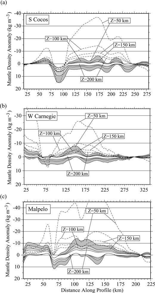
Mantle density variations along Cocos (a), Carnegie (b) and Malpelo (c) transects, inferred from the isostasy model, for different values of the compensation depth, Z= 50, 100, 150 and 200 km. Cocos and Malpelo profiles correspond to the crustal density models shown in Sallarès et al. (2003). Carnegie profile corresponds to the crustal density model from Fig. 7(a). Shaded stripes show the mantle density uncertainty inferred from the Monte Carlo analysis for each compensation depth. Dashed lines correspond to uniform crustal density models (2800 kg m−3) with the Moho geometry obtained from seismic tomography along the same transects.
Results show that the contribution of lateral crustal density variations is also significant to account for the depth anomaly. Hence, the predicted mantle density anomalies for the variable crustal density models along the three transects are negligible considering the range of uncertainty of the velocity models (between ∼0 ± 5 kg m−3 for Z= 50 km and ∼0 ± 1 kg m−3 for Z= 200 km). This means that the swell anomaly is isostatically compensated at the base of the crust and that mantle density anomalies, if present, have to be small, <5–10 kg m−3, which is under the uncertainty threshold of the method. In contrast, models considering a constant density crustal layer (even with the correct Moho geometry) predict much larger mantle density anomalies beneath the thickened part of the crust, as high as 40–50 kg m−3 for Z= 50 km in the thickest part of the Cocos and Malpelo ridges (Figs 8a and c).
In conclusion, the results show that the upper-mantle density structure beneath the GVP aseismic ridges is uniform and shows typical mantle density (∼3300 kg m−3) for a wide range of compensation depths (50–200 km), suggesting that these ridges are isostatically compensated at the base of the crust. This means that mantle density anomalies, if they once existed, are insignificant for ages greater than 10 Myr. This result is very different from that obtained by Ito & Lin (1995) based on the analysis of the gravity signatures along the present- and palaeo-axes (<8 Myr) of the CNSC. Ito & Lin (1995) corrected the gravity field for topography and for an estimated crust–mantle boundary, and they associated the remaining gravity anomaly to the presence of mantle density anomalies of thermal origin. The main difference with our work is that they assumed the lateral crustal density variations along their profiles to be negligible. However, as we have shown above, this is not the case. The inclusion of lateral crustal density variations accounts for the gravity and topography anomalies across the GVP aseismic ridges without calling for anomalous mantle densities (and temperatures). This seems to indicate that the significance of compositional mantle buoyancy as a result of melt extraction and depletion (e.g. Oxburgh & Parmentier 1977) is smaller than suggested by previous studies performed in the region (e.g. Canales et al. 2002). However, it is not straightforward to compare the work of Canales et al. (2002) with ours, because they focussed their study on the present-day axis of the CNSC, while we refer to structures formed more than 10 Ma. In any case, our results show that any estimation of the mantle density structure from gravity and topography analysis for regions showing prominent variations in crustal thickness and topography, such as aseismic ridges, would have to include a correction for lateral crustal density contrasts.
6 Nature of The GaláPagos Hotspot
The amount of melt produced by adiabatic decompression of the mantle and the composition of the resultant igneous crust are known to depend on:
- (i)
the temperature (Klein & Langmuir 1987; White et al. 1992), composition (e.g. Korenaga & Kelemen 2000) and water content (Ito et al. 1999; Braun et al. 2000) of the mantle source; and
- (ii)
the mechanical constraints bounding the extent of the mantle melting zone (i.e. the presence of a lithospheric lid; e.g. Watson & McKenzie 1990; Korenaga et al. 2002; Fig. 9a).
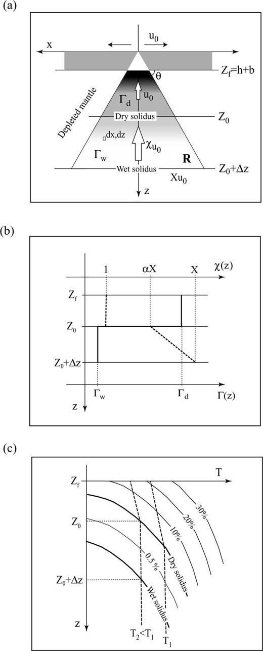
(a) Sketch summarizing the melting process for mantle corner flow beneath spreading ridges. U0 is the spreading rate and χ is the mantle upwelling ratio. In our model, χ= 1, passive upwelling, above the dry solidus. The final depth of melting is Zf, which is determined by the lithospheric lid (old lithosphere, b, and newly formed oceanic crust, h). The initial depth of melting is Z0, which is defined by the intersection of the dry solidus and the mantle adiabat. ΔZ is the thickness of the damp melting area. R is the section of the melting region for mantle corner flow, dx, dy indicate an element of mantle. (b) Diagram indicating the values of the upwelling ratio at the base of the melting zone, X, the slope of the upwelling ratio decay within the damp melting zone, α, and the melt productivity within the dry, Γd, and damp, Γw, melting regions in our melting model (see details in Sections 6.1 and 6.2). The thick solid line represents the melt productivity, Γ (z), and the thick dashed line the upwelling ratio, χ (z). (c) Scheme of a phase diagram illustrating the dry and wet solidus (thick solid lines), the mantle adiabats for different potential temperatures (dashed lines), and the melting rates for given Γd and Γw (thin solid lines).
McKenzie & Bickle (1988) demonstrated that the oceanic crust of 6–7 km thick and MORB-like composition normally originated at a spreading centre is the result of decompression melting of a mantle source composed of dry pyrolite with a potential temperature of ∼1300°C. In this case, the crustal accretion is considered to be only a passive response to seafloor spreading (i.e. passive upwelling). Higher mantle temperatures or compositional anomalies may cause buoyant upwelling of the mantle (i.e. active upwelling; e.g. Ito et al. 1996). The combination of active upwelling and higher mantle temperatures, or the presence of a more fertile mantle source, will produce larger amounts of melting and, eventually, a thicker crust. Generally, melt anomalies are considered to have a thermal origin rather than a compositional one, in accordance with the original hotspot hypothesis (Wilson 1963; Morgan 1971). Because the MgO content of melt increases as mantle temperature rises above normal and seismic velocities of igneous rocks are proportional to their MgO content, igneous crust produced by a thermal anomaly should also display higher velocity than normal oceanic crust (White & McKenzie 1989). This hypothesis works well in a number of cases and has been repeatedly invoked to explain the origin of high-velocity crustal roots found in aseismic ridges (e.g. Grevemeyer et al. 2001; Walther 2002), oceanic plateaux (Coffin & Eldholm 1994; Charvis et al. 1995; Charvis & Operto 1999; Darbyshire et al. 2000) or passive volcanic margins (e.g. Kelemen & Holbrook 1995; Barton & White 1997). However, as we stated in Section 1, two recent wide-angle seismic studies performed in the North Atlantic volcanic province (Korenaga et al. 2000) and in the Galápagos province (Sallarès et al. 2003 and this study) have shown that lower igneous crust can also have normal or lower than normal seismic velocities, thus contrary to what conventional plume theory predicts. By comparing those results with the predictions of a mantle melting model based on empirical relationships between the seismic velocity of compressional waves, and the mean pressure and fraction of melting (Korenaga et al. 2002), Sallarès et al. (2003) suggested that other parameters such as active upwelling or major element compositional anomalies can be more significant than mantle temperatures to account for the excess of melting. Another option that is not contemplated in the model of Korenaga et al. (2002) is the possible influence of deep damp melting. It has been suggested that damp melting between the dry and wet solidus for a volatile-bearing mantle (∼70–120 km deep) may constitute a significant part of the total volume of melt, even if the melting rate is an order of magnitude lower than that of dry melting (Hirth & Kohlstedt 1996; Braun et al. 2000), if it is coupled with vigorous upwelling at the base of the melting zone (e.g. Maclennan et al. 2001). Accordingly, numerical models indicate that the viscosity increase associated with dehydration prevents buoyancy forces from contributing significantly to mantle upwelling above the dry solidus, and thus the upwelling in the primary melting zone is mostly passive and the melt production consequently lowers in this zone of the melting region (Ito et al. 1999). The results of a recent geophysical and geochemical study along the CNSC suggest that deep damp melting may be the most significant factor to account for the excess of magmatism associated to the presence of the GHS (Detrick et al. 2002; Cushman et al. 2005).
In the next section, we develop a mantle melting model including the effect of mantle temperature, deep damp melting, active upwelling beneath the dry solidus and mantle source composition, in order to quantify the relative significance of the different melting parameters on the seismic structure of the resultant igneous crust. The final purpose is to compare the results with those obtained in the different aseismic ridges of the GVP in order to determine the most plausible nature of the GHS.
6.1 Mantle melting model
Our mantle melting model is based on that previously developed by Korenaga et al. (2002), in which a connection between the parameters describing mantle melting processes and the resultant crustal structure is established on the basis of an empirical relationship between crustal velocity and the mean pressure and degree of melting. They considered a 1-D steady-state melting model including the effects of mantle potential temperature, active upwelling and considering the presence of a lithospheric lid. The main differences between their model and ours are as follows:
- (i)
we consider a 2-D steady-state model to describe the triangular melting regime resulting from mantle corner flow (e.g. Plank & Langmuir 1992);
- (ii)
we calculated the mean degree of melting as the average degree of melting of all the individual parcels of melt pooled in the crust (Forsyth 1993; Plank et al. 1995);
- (iii)
we included the effect of deep damp melting (Hirth & Kohlstedt 1996; Braun et al. 2000); and
- (iv)
we restricted active upwelling to beneath the dry solidus, according to the calculations of Ito et al. (1999).
Our model does not represent a rigorously based physical model; it is only an approximation to estimate the relative importance of the different parameters that characterize the mantle melting process. We have chosen this model representative of melting beneath an oceanic ridge because four of the five profiles that we have modelled correspond to aseismic ridge segments that were emplaced at the spreading axis as a result of hotspot–ridge interaction (Sallarès & Charvis 2003). The only exception is the southern Cocos profile (Fig. 8a), which is probably the result of an initial phase of on-ridge emplacement of a thicker than normal crust (∼13 km), and a second phase of off-ridge thickening (∼3.5 km) when the aseismic ridge passed over the GHS at ∼100 km from the CNSC axis (Sallarès & Charvis 2003). In any case, the melting model can be extrapolated to an intraplate environment by considering the presence of a lithospheric lid limiting the extent of the mantle melting region. The definition and values of all constants and variables used in the model are given in Table 2.

 , can be found by integrating the melt production rate,
  , of an element of mantle over the cross-sectional area in which melting occurs, R (Fig. 9a). We have chosen the simplest triangular melting region, in which the angle of the lithospheric boundary with respect to the horizontal, θ, is 45° (Fig. 9a; Ahern & Turcotte 1979). The melt production rate is the product of the melt productivity, Γ, and the upwelling rate, w, which we define to be the product of the spreading rate, u0, and the upwelling ratio, χ:
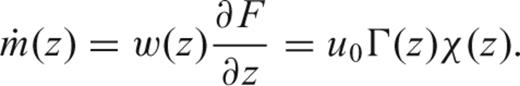
 is given in terms of melt fraction by weight, it is necessary to add a correction factor (ρm/ρc) to account for the difference between crustal and mantle densities. Considering the model parameters as defined in Fig. 9 and integrating for the mantle melting zone, R, we obtain
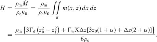
 , is the integral over the whole melting region of the product of the melt production rate and the degree of melting at a given parcel of mantle, divided by the total melt production (Forsyth 1993):
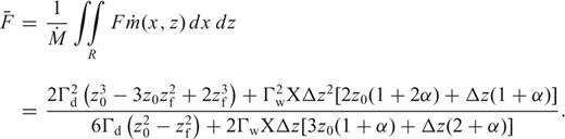

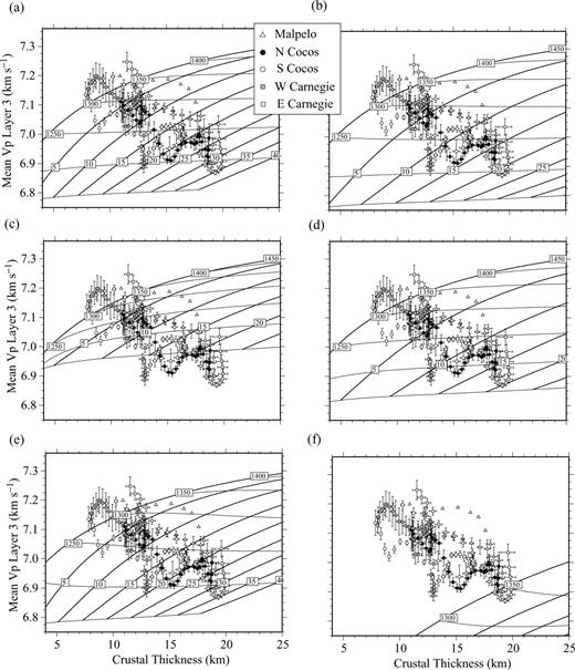
H–Vp diagrams corresponding to different melting parameters. Crustal thickness is plotted versus mean layer 3 velocity. Values are taken from the velocity models estimated along the five profiles indicated in Fig. 1. Southern Cocos (white circles), northern Cocos (solid circles) and Malpelo (triangles) correspond to the models shown in Sallarès et al. (2003). Western Carnegie (shaded squares) and eastern Carnegie (white squares) correspond to the models shown in Fig. 3. Thin lines correspond to the mantle potential temperatures and thick lines indicate the upwelling ratio at the base of the mantle melting zone. Melting parameters: (a) Γd= 15 per cent GPa−1, Γw= 1 per cent GPa−1, α= 0.25, ΔZ= 50 km, pyrolitic composition; (b) Γd= 15 per cent GPa−1, Γw= 1 per cent GPa−1, α= 1, ΔZ= 50 km, pyrolitic composition; (c) Γd= 15 per cent GPa−1, Γw= 1 per cent GPa−1, α= 0.25, ΔZ= 75 km, pyrolitic composition; (d) Γd= 15 per cent GPa−1, Γw= 2 per cent GPa−1, α= 0.25, ΔZ= 50 km, pyrolitic composition; (e) Γd= 20 per cent GPa−1, Γw= 1 per cent GPa−1, α= 0.25, ΔZ= 50 km, pyrolitic composition; (f) same as (e) but with a source composed of 30 per cent MORB and 70 per cent depleted mantle. See details in Section 6.2.
6.2 Comparison with velocity models
In order to compare the results predicted by the model with those estimated from wide-angle seismics, we have calculated the long-wavelength crustal structure along the different velocity models obtained at the Carnegie (Fig. 3), Cocos and Malpelo ridges (Sallarès et al. 2003). Given that the remaining porosity and alteration of oceanic layer 3 are likely to be small, as suggested by the low-velocity gradient, its average seismic velocity is considered to be a good proxy of the seismic velocity of the igneous crustal rocks (e.g. Kelemen & Holbrook 1995; Korenaga et al. 2000). Thus, we have calculated the long-wavelength crustal structure by averaging the layer 3 velocity (Vp) and crustal thickness (H) within a 25-km-wide laterally moving window along the different transects. Uncertainties of model parameters obtained from the Monte Carlo analysis (Fig. 4) are used to assign error bounds to both H and Vp. Because standard H–Vp diagrams are calculated at particular P–T conditions (400 °C, 600 MPa), we corrected Vp from the in situ conditions to this reference state, following the approach described in Sallarès et al. (2003). The corrected results along all the GVP profiles are represented in the different diagrams obtained using different combinations of the melting parameters, which are shown in Fig. 10. Note that the overall anticorrelation between lower crustal velocity and crustal thickness systematically obtained in the ridges is clearly observed in the H–Vp diagrams.
Fig. 10(a) show the H–Vp diagram obtained using a linear melting function with Γd= 15 per cent GPa−1 and Γw= 1 per cent GPa−1. The thickness of the damp melting zone, Δz, is 50 km (e.g. Braun et al. 2000), and α= 0.25, to be consistent with the 4–5 fold increase of the mantle viscosity between the wet and dry solidus for a water content comparable to the MORB source (Ito et al. 1999). This set of parameters defines our reference model. H and Vp are calculated for mantle potential temperatures varying from 1150 to 1450 °C, and an upwelling ratio at the base of the damp melting zone, X, varying from 1 to 40. Note that, in this case, the seismic structure of the thinnest oceanic crust (i.e. that of the normal oceanic basins) is consistent with that expected for a crust generated by passive decompression melting of dry pyrolitic mantle (X∼ 1) with a potential temperature of 1300–1350 °C, which is in agreement with the estimates of McKenzie & Bickle (1988). On the contrary, the seismic structure of the thickest crust would require extremely vigorous upwelling (X∼ 30–35) of colder than normal mantle (Tp= 1175–1200 °C). It seems difficult to imagine a physical process compatible with this result. In the second test (Fig. 10b), we considered a uniform upwelling ratio within the damp melting zone (α= 1). The result does not change excessively in terms of estimated potential temperatures and the only difference is that the upwelling ratio would have to be somewhat smaller (X∼ 20) to explain the crustal structure of the thickest segments. In the third test (Fig. 10c), we explored the influence of a thicker damp melting zone (Δz= 75 km). The result is even worse, because the potential temperatures required to explain the crustal thickening must be lower than those estimated for the reference model (Fig. 10a). In the fourth test (Fig. 10d), we considered a higher melt productivity in the damp melting zone (Γw= 2 per cent GPa−1). Again, the result does not change in terms of estimated potential temperatures for the thicker crust (Tp∼ 1150 °C) and the maximum upwelling ratio would have to be X∼ 15. Finally, we performed another test (Fig. 10e) considering a higher melt productivity within the primary melting zone (Γd= 20 per cent GPa−1), but the only effect that is visible is the lower potential temperatures required to explain the crustal structure of the oceanic basins (Tp < 1300 °C). Therefore, the main conclusion of these tests is that it seems difficult to explain the seismic structure of those aseismic ridges considering only deep damp melting coupled with active upwelling. Low mantle potential temperatures would be always required, which is both counter-intuitive and difficult to justify.
6.3 Discussion
A plausible qualitative explanation of the low crustal velocities could be the occurrence of subcrustal fractionation beneath the ridge axis. The loss of high-velocity minerals as material upwells may reduce seismic velocities of the resulting crust in comparison with that resulting from crystallization of a primary, mantle-derived melt. However, it has been shown that the effect of subcrustal fractionation on seismic velocities is only significant for velocities at least 10 per cent higher than those obtained in the lower crust of the Carnegie ridge (Korenaga et al. 2002).
Another alternative that must be examined is the presence of compositional anomalies in the mantle source. Isotopic and trace element geochemistry of basalt samples from the Galápagos platform(White et al. 1993; Blichert-Toft & White 2001; Harpp & White 2001), the present-day axis of the CNSC (Verma et al. 1983; Schilling et al. 2003), the Cocos, Carnegie and Malpelo ridges (Hoernle et al. 2000; Geldmacher et al. 2003; Werner et al. 2003), and the Caribbean large igneous province (CLIP; Hauff et al. 2000) indicate that the mantle source of the GHS may be internally heterogeneous. The Pb, Hf, Nd and Sr isotopic composition of CNSC lavas suggests the presence of at least two major components for the GHS mantle source, probably corresponding to a recycled mix of oceanic crust—lower-mantle material and to recycled continental-derived material or pelagic sediment (Schilling et al. 2003). Basalts from the Galápagos platform show greater scatter in the isotope space, displaying an east facing horseshoe spatial pattern characterized by four main domains (White et al. 1993; Harpp & White 2001). The same domains are clearly observed in the Cocos ridge near the subduction zone, indicating the existence of a complex spatial zonation of the GHS magmatism for at least 14 Myr (Hoernle et al. 2000). Rocks from the eastern, southern and northern Galápagos domains have enriched signatures reflecting mixtures of depleted MORB source material with different types of altered recycled oceanic crust (Hauff et al. 2000). The central Galápagos domain contains the highest 3He/4He ratios, indicating that the source is probably enriched with deep, undegassed mantle material (e.g. Graham et al. 1993; Blichert-Toft & White 2001). Likewise, Sr-Nd-Pb isotope and trace element signatures from the CLIP, which is believed to represent the onset of the GHS, are consistent with the derivation from a mixture of a depleted mantle source and recycled oceanic crust (Hauff et al. 2000).
Basalts from the GVP also display anomalies in incompatible and major elements with respect to normal MORB. Geochemical data show that lavas from the Galápagos platform have similar Na2O, lower SiO2 and slightly higher FeO than do MORB at similar MgO concentration (White et al. 1993). In the case that the plume and the asthenosphere have similar major element composition, these observations suggest that the depth of melting is slightly greater to that of melting beneath mid-ocean ridges, but the degree of melting is similar, which is somewhat surprising if the mantle temperatures associated with the hotspot are higher than normal. Fe8 values (total Fe content as FeO corrected to 8 wt per cent MgO) are highest in the central islands (with values higher than 13 for individual samples) and lowest in the southern and northwestern ones, suggesting deeper melting beneath the central part of the platform (Geist 1992; White et al. 1993).
In the CNSC, lavas sampled away from the zone of maximal GHS influence show Fe8 values higher than 11 (e.g. at the 87°–88° W segment), which are relatively elevated for their axial depth (∼2200 meters below seafloor; Christie et al. 2005). However, the correlations of Fe8 and Na8 (total Na content as Na2O corrected to 8 wt per cent MgO) with axial depth and crustal thickness along the GHS-influenced segment of the CNSC are different to those of the global MORB array, the thickest crust and shallowest axial depth being characterized by the lowest Fe8 and the highest Na8 (e.g. Klein & Langmuir 1987; Langmuir et al. 1992; Christie et al. in press; Cushman et al. 2005). The Fe8 decrease and Na8 increase along the CNSC as we approach the GHS contradict apparently with the presence of a hotter mantle, as increasing potential temperature would have to lead to deeper melting and higher FeO, as well as to a higher extent of melting and lower Na2O, at a given MgO. Asimow & Langmuir (2003) explained the apparent discrepancy between mantle temperature and Fe8 in terms of water addition to the mantle source. They showed that one of the dominant effects of water is the suppression of plagioclase crystallization, which leads to lower FeO contents in fractionated liquids compared with anhydrous melting. Likewise, Cushman et al. (2005) showed that hydrous melting may also account for the observed correlation between Na8 and crustal thickness, suggesting that melting of a deep, hydrous root is the dominant process to account for the geophysical and geochemical variations along the western CNSC. Damp melting alone does not explain, however, the higher Fe8 values observed in the volcanoes of the central Galápagos platform as compared with the southern (and northern) ones (Geist 1992; White et al. 1993), and the high Fe8 values of the easternmost CNSC segments (Christie et al. in press). Normally, one would expect to have low Fe8 values also at the zone of maximal hotspot influence (beneath the platform). However, this is not the case, which may indicate either (i) the influence of deep damp melting is not significant beneath the platform, or (ii) the mantle melting source is somehow enriched in iron.
The model described in Section 6.1 is only valid for mantle compositions similar to pyrolite, because the relationship between seismic velocity and melting parameters used in this study (Korenaga et al. 2002) was estimated for this model composition only. The uniform composition of most ocean peridotites is well explained by melting of a pyrolitic mantle and thus the assumption of a uniform pyrolitic mantle is probably justified in most cases. Nevertheless, the presence of major element heterogeneities in the mantle source has been suggested in some special cases, namely the generation of large igneous provinces and flood basalts (e.g. Campbell 1998). In particular, Korenaga & Kelemen (2000) suggested that most of the magmatism of the North Atlantic igneous province may be owing to a relatively Fe-rich mantle source (Mg #∼0.87) with respect to the normal MORB source (Mg #∼ 0.90), and they indicated that such a source could be a mixture of depleted upper mantle and ancient, recycled oceanic crust, which is similar to that proposed for the GVP and the CLIP based on isotopic and trace element geochemistry (Hauff et al. 2000; Hoernle et al. 2000; Harpp & White 2001; Schilling et al. 2003). Based on the results of an experimental study of the phase and melting relations of homogeneous basalt and peridotite mixtures, Yaxley (2000) showed that the lower solidus and compressed solidus–liquidus temperature interval of material containing a few tens of per cent basalt in peridotite may combine during mantle upwelling to substantially enhance melt production. Hence, he suggested that mixtures of recycled oceanic crust and peridotite in mantle plumes may provide a plausible source for extra melting (as previously suggested by Cordery et al. 1997), and that the resulting primary melting liquids would have to show higher than normal Fe/Mg values (lower Mg #).
However, too few melting experiments with source compositions different from pyrolite exist to develop a quantitative model including the effect of source heterogeneities. Korenaga et al. (2002) performed a preliminary attempt to illustrate the potential effect of a major element heterogeneity such as that described for the North Atlantic province. They considered a hypothetical source composed of 70 per cent depleted pyrolitic mantle (Kinzler 1997) and 30 per cent MORB (Hofmann 1988; Mg #∼ 0.86), calculated isobaric batch melts, and derived a relationship between the norm-based velocity (see definition in Korenaga et al. 2002) and the melting parameters. Similarly, we have performed a final test with our model using the same relationship combined with a higher melt productivity in the primary melting zone (20 per cent GPa−1) and a 50 °C lower temperature in the solidus with respect to normal pyrolite in order to reflect the Fe enrichment (Fig. 10f). These modelling results indicate that the seismic structure of the thickest crustal segments can be more easily explained by passive to moderately active upwelling of a normal temperature but fertile mantle source rather than by that of a hot and homogeneus pyrolitic mantle, even if vigorous upwelling of a hydrous mantle root is included in the model. This is in agreement with that previously suggested by Sallarès et al. (2003) based on the velocity–thickness anticorrelation obtained in Cocos and Malpelo.
Melting of recycled subducted oceanic crust in the mantle source could thus explain qualitatively the observed isotope and trace element patterns, as well as the crustal thickening and the anticorrelation between crustal thickness and layer 3 velocity of the aseismic ridges, without the need to consider anomalously high mantle temperatures. As we stated above, the isotopic composition of CNSC, GVP and CLIP lavas seems to indicate the presence of a component corresponding to a recycled mix of oceanic crust and lower-mantle material (Hauff et al. 2000; Hoernle et al. 2000; Schilling et al. 2003), which could potentially lead to deeper melting, enhanced melt production (i.e. a thicker crust) and relatively high FeO values for a given MgO (e.g. Yaxley 2000). This is generally consistent with the FeO trends observed in the Galápagos archipelago (White et al. 1993), but we suggest that the occurrence of deep damp melting may probably smooth or even counterbalance this tendency, especially along the CNSC. The Sm-Nd and U-Pb isotope systematics indicate that the CLIP source components were separated from a common depleted MORB source <500 Myr before CLIP formation (90–100 Ma), which has been interpreted to reflect the recycling age of the oceanic lithosphere (Hauff et al. 2000). These authors propose large volume contamination of the upper mantle with young recycled oceanic lithosphere by means of multiple mid-Cretaceous starting plume heads (e.g. Hanan & Graham 1996) as a plausible origin for the mantle source heterogeneity of the GHS. In addition, a contribution of extra melting from a deep and hydrous root is probably needed to account for the high Na8 and low Fe8 values along the most GHS-affected segment of the CNSC (Asimow & Langmuir 2003; Cushman et al. 2005). The relative significance of fertile versus damp melting is however difficult to quantify, owing to the lack of available mantle melting experiments using model compositions different from pyrolitic.
One aspect difficult to reconcile with the hypothesis of basalt addition to the mantle source prior to melting as the origin of the GVP concerns the upwelling mechanism of the denser mantle heterogeneity in the absence of a thermal plume. It is clear that present upwelling beneath the Galápagos archipelago can not be simply a passive response to seafloor spreading. The Galápagos platform is too far away from the CNSC, so it is necessary to have a source of active upwelling to explain the current hotspot volcanism. If we rule out the presence of a thermal anomaly (which, if present, must be weak, just a few tens of degrees according to Cushman et al. 2005), mantle upwelling must be associated either with compositional buoyancy or with the presence of any other type of sublithospheric convection. Subducted oceanic crust is denser than normal pyrolitic mantle above the bottom of the mantle transition zone (Ringwood & Irifune 1988), so it will tend to lie at this level of neutral buoyancy unless it is sent back to the surface by a rising stream. A plausible mechanism that has been shown to be capable of bringing up dense fertile mantle without a thermal anomaly is sublithospheric convection driven by surface cooling (Korenaga 2004). This model has been proposed to explain the origin of continental breakup magmatism of the North Atlantic volcanic province, but it is apparently more difficult to associate the GHS volcanism to a similar process. An alternative that must be examined in order to explain active upwelling is the effect of water content on mantle buoyancy. It has been shown that the presence of water in the mantle source reduces substantially mantle viscosity and enhances mantle flow, increasing, in turn, the mantle upwelling rates (Ito et al. 1999), but the direct effect of water content on density variations and buoyancy is not constrained so far.
7 Summary and Conclusions
We have estimated the crustal structure of the Carnegie ridge from refraction/reflection traveltime tomography along two wide-angle seismic transects located over ∼20 and ∼11.5 Myr old seafloor over the Nazca Plate at the GVP. The crust shows a typical oceanic structure, composed of an upper layer characterized by striking velocity gradients (i.e. the oceanic layer 2) and a lower layer showing much more uniform velocity (i.e. the layer 3). However, the crust is much thicker than normal. In profile 1 (Fig. 1), maximum crustal thickness is around 13 km, thus it is twice the thickness of normal oceanic crust, while in profile 2 it is around 19 km. In both profiles, layer 2 thickness is quite uniform (3–4 km) regardless of total crustal thickness variations, indicating that the excess of melting provided by the GHS is mainly accommodated by layer 3. The velocity structure obtained across the Carnegie ridge is almost identical to that previously estimated at the conjugate profiles of the Carnegie ridge ones over the Cocos and Malpelo ridges, and in another one across the Cocos ridge over ∼15 Myr old seafloor (Sallarès et al. 2003). This suggests that all the volcanic edifices of the GVP are probably the product of a single, long-lasting mantle melting anomaly, in conjunction with a regular process of ridge edification, which has been active for at least the last 20 Myr. A recent study based on all these data has shown that the crustal thickness variations at the different GVP aseismic ridge segments are the effect of temporal variations in the relative location between the CNSC and the GHS, and not that of temporal GHS intensity variations, indicating that the anomaly is additionally a stable and unvarying mantle feature (Sallarès & Charvis 2003). The estimated crustal velocity models along the different transects are also consistent with gravity and bathymetry data. The velocity-derived density models show that Carnegie, Cocos and Malpelo have uniform normal upper-mantle densities, indicating that GVP aseismic ridges are isostatically compensated at the base of the crust. Therefore, there is not compelling evidence for the presence of upper-mantle density anomalies, indicating that such mantle anomalies, if present when the ridges were originated, are not significant for ages older than 10 Myr.
A remarkable feature that is systematically observed in all the aseismic ridges is the overall anticorrelation between layer 3 velocities (and densities) and total crustal thickness. A 2-D steady-state mantle melting model based on that of Korenaga et al. (2002) is developed and used to illustrate that it is very difficult to account for the seismic structure of the GVP ridges if it is assumed that the source of the GHS is a thermal anomaly, even if vigorous mantle upwelling coupled with deep damp melting is included in the model. It seems easier to account for the estimated crustal structure if a more drastic, major element heterogeneity, is also considered in the melting model. Based on these results, we suggest that the primary source of the GHS is a compositional heterogeneity, which may represent a mixture of depleted mantle and recycled oceanic crust (e.g. Yaxley 2000). Such a mantle source explains well the isotope and trace element patterns showed by GVP and CLIP basalts (Schilling et al. 1982; Hauff et al. 2000; Schilling et al. 2003). Additional deep and hydrous mantle melting is probably needed to account for the high Na8 and low Fe8 observed in the most GHS-affected segment the CNSC (Detrick et al. 2002; Asimow & Langmuir 2003; Cushman et al. 2005). Mantle melting experiments for mantle source compositions different from pyrolitic are though required to quantify the relative significance of fertile versus damp melting to account for the origin of the GVP.
Acknowledgments
The SALIERI-2001 experiment was funded by the German Ministry of Education, Research, Science and Technology (BMBF) under project no. 03G0159A. The French scientific party was supported by IRD, Institut National des Sciences de l'Univers (INSU) and French Research Institute for Exploitation of the Sea (IFREMER) through ship time exchange. VS was financially supported by a grant from the Marie Curie Fellowship EU programme, contract no. HPRI–CT–1999–00037, during the time the work was conducted. We thank the Associate Editor, Jean Francheteau, as well as the reviewers Juan Pablo Canales and Jun Korenaga, for their constructive reviews, which helped to improve substantially the original version of the manuscript. We are also indebted to H. Andersen, master of the R/V Sonne, and to the crew of the vessel for their professional support and the good working atmosphere during the cruise. This is Géosciences Azur contribution no. 640.
References
Author notes
Now at: Unitat de Tecnologia Marina—CMIMA—CSIC Passeig Marítim de la Barceloneta 37–49, 08003 Barcelona, Spain. E-mail: [email protected]
The SALIERI Scientific Party: W. Agudelo, A. Anglade, A. Berhorst, N. Bethoux, A. Broser, A. Calahorrano, J.-Y. Collot, N. Fekete, A. Gailler, M. A. Gutscher, Y. Hello, P. Liersch, F. Michaud, M. Müller, J. A. Osorio, C. Ravaut, K. P. Steffen, P. Thierer, C. Walther, B. Yates.
