Optimal parametrization of tomographic models Free

Summary

1 Introduction

In this paper, we address the question of optimizing the parametrization of the Earth for the purpose of tomographic inversions. We shall assume that the tomographic data d_i (i= 1, …, M) are linearly related to the earth model m(r) as

1

where F_i(r) is a Fréchet kernel. The problem needs invariably to be discretized. Although one may postpone discretization to a later stage (Tarantola & Nercessian 1984), here we assume from the outset that the model is described by a finite number of parameters m_j, (j= 1, …, N):

2

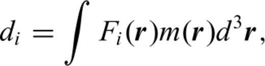
The possibility of a choice for the basis functions h_j has led to various inversion philosophies. Backus & Gilbert (1967) choose the Fréchet kernels F_i themselves as a basis, thus avoiding that unwarranted detail is introduced in the solutions by using basis functions that may be orthogonal to the Fréchet kernels and thus in the null space of eq. (1). This leads to a problem if ray theory is used to model traveltimes because the support for F_i is infinitely narrow along a ray. In one dimension, this problem can be solved through integration by parts (Johnson & Gilbert 1972), but in higher dimensions it is easier to convolve the ray kernel with an empirical smoothing function (Michelena & Harris 1991) or to reject ray theory in favour of the more accurate finite-frequency theory (Dahlen et al. 2000).

The advantage of this approach, the choice of the minimum norm solution, is also its greatest weakness: by concentrating non-zero model values in areas that are well resolved, unresolved areas may show up as zero patches within the model that can easily be mistaken for structure. Alternative inversion strategies have therefore sought to dampen unwarranted detail by searching for a model that is smoothest in some sense.

Dziewonski et al. (1975) pioneered the use of low-order spherical harmonics in global tomographic inversions. The most recent inversions of this kind (e.g. Boschi & Dziewonski 1999) use spherical harmonics up to degree 40. This allows us to image detail with scale lengths as small as 500 km. Whereas in some areas this may oversample the available resolution, in regions such as subduction zones the structure of geophysical interest is of smaller scale and the high seismicity allows for at least some of this detail to be resolved in local studies (e.g. Papazachos & Nolet 1997).

Although the spherical harmonics expansion is highly compatible with the usual modelling of other geophysical variables, such as the gravity and magnetic field, or the geoid, and therefore the preferred approach in many global geodynamics studies, the inflexibility of the spherical harmonic expansion to adapt to local variations in resolution is a drawback. Inversions to regularize high angular orders by a locally varying smoothness condition are possible in principle, but awkward to implement and we know of no efforts to push the resolving power to a level that is sufficient to image, e.g. upper-mantle slabs.

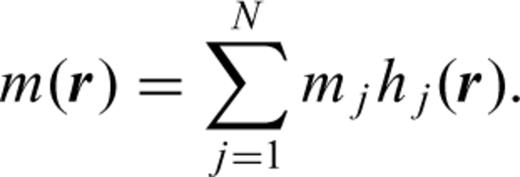
Local interpolation schemes are more readily adaptable to handle the often extreme variations in resolution, in particular the schemes that rely on Delauney meshes, optimized tetrahedral interpolation grids (Lawson 1977; Watson 1981), which were introduced in geophysical modelling by Sambridge et al. (1995) and Sambridge & Gudmundsson (1998). In contrast to regular grids, such as the 2°× 2° grid used by Van der Hilst et al. (1997), interpolation supports can be spread out and concentrated to match the resolving power. The idea to use the resolving power in this way was first expressed by Wiggins (1972) and has obvious advantages. This becomes immediately clear by studying the modelling of a continuous one-dimensional (1-D) scalar function f(x), parametrized by its value at N locations x_i and constrained by M data points f_j=f(x_j) =d_j (Fig. 1). This example is taken from VanDecar & Snieder (1994), who give an extensive account of the convergence problems posed by smoothing operators. However, in this particular case, the most natural solution, in the sense of the solution with the least unwarrant detail, is to connect the data points f_j by straight lines. In other words, we should parametrize the model with only M nodes, suitably located where we resolve f(x) exactly. Note that the minimum norm solution of a parametrization with N ≫ M would yield a model of M distinct spikes and leave all non-specified f(x_i) zero.

Figure 1

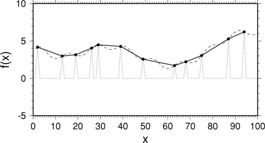
Example of the interplay between parametrization, smoothing and damping (after VanDecar & Snieder 1994). A continuous function f(x) is sampled at 12 locations x_i. The inverse problem is to reconstruct the function from these samples. The minimum norm solution that satisfies is given by the dotted line. If we force the solution to be smooth by fitting a low-order harmonic, we obtain the dashed curve. The solid curve is the solution obtained by adapting the parametrization to the resolution, choosing as gridpoints those x_i where f is specified and imposing a linear behaviour in between.

Open in new tabDownload slide

The philosophy followed in this example can be extended to multidimensional inverse problems and, in fact, this approach has dominated Western science in one form or another since William of Occam formulated his celebrated principle that the simplest hypothesis is the preferred one (e.g. Constable et al. 1987). Backus (1970) searched for those linear properties or quellings (i.e. weighted averages) of the model that can be uniquely determined, but his approach is not feasible for large tomographic inversions. The same drawback applies to methods based on information theory that try to maximize the entropy on the mean (Rietsch 1977; Maréchal & Lannes 1997). However, we may obtain a result satisfying the same basic principle, if we realize that unresolved structure is what it says it is, i.e. it may or may not be there, and we would violate the basic principles of science if we were to allow detail to creep into the solution that is unwarranted: hence, our approach to choose a parametrization that is adapted to resolved structure and to interpolate smoothly (e.g. linearly) in between. This point of view can be seen as a three-dimensional (3-D) extension of approach of Wiggins (1972), who adapts the thickness of layers in a 1-D inversion to the resolution at depth.

By explicitly specifying the local resolution in the formulation of an optimization problem, this approach differs from many current attempts at reparametrization (see Sambridge & Rawlinson 2005, and references therein).

2 A Minimum Energy Parametrization Strategy

We assume we know the resolution, even if only approximately (see the discussion in Section 6 for various ways to obtain resolution estimates). That is, at every location r in space we assign a resolving length ℓ (r) and we shall wish to space nodes near r at a distance close to this resolving length ℓ (r).

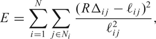
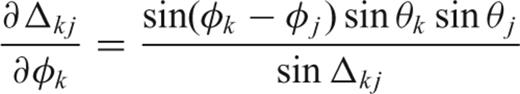
Each node has a set of natural neighbours for which we shall apply our distance criterion; i.e. if is the set of natural neighbours of node i, we shall wish to minimize the penalty function:

3

where L_ij is the actual distance between nodes i and j, and ℓ_ij the average resolving length between i and j. Physically, we can imagine node pairs (i, j) to be connected by springs of length ℓ_ij and spring constant ℓ⁻²_ij. E in eq. (3) is then twice the potential energy of this system and will be zero when nodes are spaced exactly at distances ℓ_ij. The variable spring constants in the denominator have been introduced to avoid that long springs have a weight in the minimization that is out of proportion when compared with short springs.

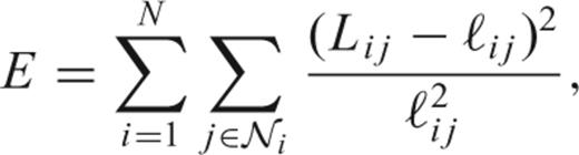
The natural neighbours are defined by a 3-D extension of the empty circumcircle criterion (Watson 1981, 1992; Sambridge et al. 1995). The 3-D version of this criterion states that the four vertices of a tetrahedron in a Delauney grid are located on a sphere. Other nodes may be located on the same sphere but no other nodes of the grid may lie within the sphere. Each node is located on several such spheres and the collection of all nodes on the spheres common to one gridpoint constitutes its set of natural neighbours. The resulting mesh is named a Delauney mesh. It can be constructed using readily available software, such as the command triangulate in the Generic Mapping Tools (gmt; Wessel & Smith 1995) or the qhull program distributed by the Geometry Center of Minneapolis (Barber et al. 1996). For the examples in this paper, we have used qhull. The outer shell of a Delauney mesh must be convex and is named the convex hull. In a spherical Earth, the hull may consist of two spherical surfaces, for example if we exclude the core. To ensure that the hull maintains its convex character, the nodes on the hull are kept fixed once they have been established.

The number of nodes available to minimize E determines how close we can get to the ideal solution E= 0. We estimate the optimal number of nodes by assuming that the tetrahedra are equilateral with sides ℓ(r) and that the resolution in the Earth has a probability density P(ℓ). The volume of an equilateral tetrahedron with side ℓ is equal to

4

The average volume of a tetrahedron in an Earth with a probability distribution P(ℓ) for resolving length is

5

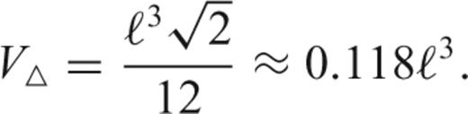
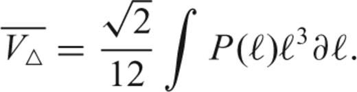
If we fill a volume V_⊕ with N tetrahedrons, then an estimate for the optimal value for N is given by . The value of N is only approximate because, in practice, the tetrahedra will not be equilateral, but the precise value of N is not critical because the resulting node spacing depends on it as N^1/3: a factor of 2 in the number of nodes will only change the average node spacing by 26 per cent.

The minimization is performed using a conjugate gradient algorithm. The gradient of E is easily found. We use Cartesian coordinates (x_i, y_i, z_i) for the node located at r_i. For the derivative of the energy with respect to x_k, we find:

6

where

7

so

8

and similar expressions for the derivatives with respect to y_k and z_k. A damping factor could easily be added to these gradients, but in our experiments we found no need for this.

For the construction of the convex hull, we force the points to lie on a sphere of radius R and spherical coordinates θ, φ are more appropriate. For large R, we may use the great-circle distance rather than the line-of-sight distance:

9

10

11

where

We find the derivatives of Δ_kj by differentiating this expression with respect to longitude φ and colatitude θ:

12

and

13

3 Starting Configuration

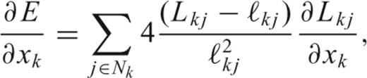
The optimization problem is non-linear because of three factors: the definition of the energy itself by eq. (3) is non-linear, the resolution ℓ_ij depends on the coordinates of neighbouring points i and j, and the Delauney meshing is non-linear; nodes may swap partners as they migrate away from their starting positions. Unless the resolution is very heterogeneous, leading to rapidly fluctuating ℓ_ij, the Delauney meshing is the most serious source of non-linearity. This introduces the danger of getting stuck in a local minimum that is not an acceptable configuration, even if we allow for a slight degree of non-optimality in the node configuration.

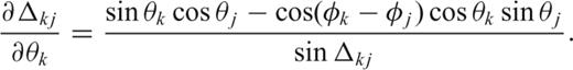
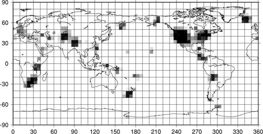
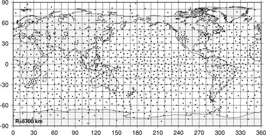
As an example, Fig. 2 shows the starting configuration for a convex hull at R= 6700 km obtained by randomly placing nodes on the sphere and Fig. 3(a) shows (hypothetical) target resolving length that is rapidly changing. We apply the conjugate gradient algorithm with a fixed Delauney mesh until it has converged (inner-loop iterations), then recalculate the mesh for the new coordinates. Repeating this in an iterative fashion (outer loop), we find the system to converge quickly in every inner loop and in four outer-loop iterations to the configuration shown in Fig. 4. The energy of this system has been reduced to 24.9 per cent of that in Fig. 2, but even though the system has node concentrations in the western US, and at the sites of dense PASSCAL experiments in Bolivia and South Africa, the densification of these nodes has been obtained at the expense of neighbouring nodes drawn into the cluster, leaving large open spaces, e.g. in the central US or just off the coast of California and Chile/Peru. To bring more nodes into the empty regions involves stretching springs too far, forcing us to cross a ridge of higher energy, a feat that the conjugate gradient method cannot accomplish.

Figure 2

Random starting configuration of nodes at the convex hull, a surface located at R= 6700 km.

Open in new tabDownload slide

Figure 3

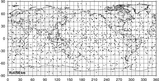
The target resolution near the surface has regions of high resolution (ℓ_ij= 300 km, black) superimposed on a background resolution of 800 km (white). The greyscale is linear.

Open in new tabDownload slide

Figure 4

The node configuration obtained for the random start configuration shown in Fig. 2.

Open in new tabDownload slide

Rather than taking recourse to methods of non-linear optimization that can overcome local minima but that are usually inefficient with large numbers of parameters, such as simulated annealing, we use a construction method of the starting grid to ensure that the starting configuration is close enough to the global minimum for an acceptable mesh to result with little effort from the optimization. The method we use is that of tessellation of a sphere, whereby triangles are subdivided until we are within a factor of of the locally desired node spacing (e.g. Constable et al. 1993; Wang & Dahlen 1995; Chiao & Kuo 2001). Fig. 5 shows the tessellation of the sphere conforming to the same target resolving lengths shown in Fig. 3. Note that we provide a dense set of nodes where needed without leaving open spaces. Convergence to the final configuration is very fast at first and slower after the third iteration (Fig. 6). Although we could have iterated further, we stopped at the configuration shown in Fig. 7. Attempts to speed up convergence using simulated annealing (by randomly perturbing node locations in between iterations over distances of the order of 10–50 km) in this example only led to the same energy and a configuration of nodes that looked visually the same, but required in fact longer CPU times. In some 3-D cases, we have noted, however, that a mild degree of annealing may be useful to escape from an undesirable local minimum.

Figure 5

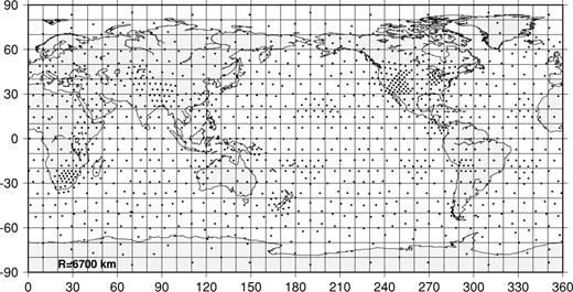
The starting configuration obtained by subdividing an initial configuration of triangles on the sphere, such that the sides of the triangles are within of the desired length.

Open in new tabDownload slide

Figure 6

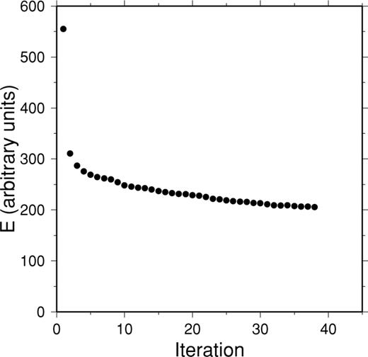
Convergence of the two-dimensional (2-D) optimiziation for the convex hull at R= 6700 km.

Open in new tabDownload slide

Figure 7

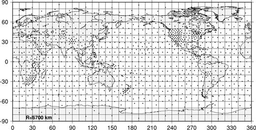
The optimal configuration obtained from the starting configuration shown in Fig. 5.

Open in new tabDownload slide

4 Application to a Realistic Resolution

We estimated the resolution for a global data set of 69 079 S waves 26 337 SS−S and 13 856 ScS−S differential traveltimes using a logarithmic relationship between the column sum of the tomographic matrix and the resolving length at the location of that parameter, using the finite-frequency matrix computed for a more random parameter distribution as in Montelli et al. (2003). The resolving length obtained in this way was loosely calibrated to the results of resolution tests, but remains approximate. Our only aim here is to show how the method works for a realistic data set.

We again proceeded to construct the convex hull at R= 6700 km. A similar surface was constructed at the depth of the core–mantle boundary (CMB, 3480 km). The latter surface is, strictly speaking, not a convex hull, because the Delauney mesh extends into the core. It may, however be ignored if the tomography is confined to the mantle. If the tomographic model is allowed to be discontinuous across boundaries such as the CMB, one could introduce pairs of nodes on both sides of the surface, but it will be more straightforward to construct separate meshes for mantle, core and inner core. Those for the mantle and core would have a phantom mesh below their lower boundary, which is never used. The results are shown in Fig. 8.

Figure 8

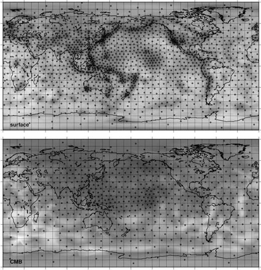
Top: the model nodes of the convex hull, adapted to the near-surface resolution of a set of long period S, SS and ScS cross-correlation arrival times interpreted using finite-frequency theory. The greyscale shows the target resolution, ranging from 0 km (black) to 1500 km (white). Bottom: the bounding surface of the model at the depth of the core–mantle boundary (CMB). The greyscale is as in the top figure.

Open in new tabDownload slide

After constructing the convex hull, we construct a starting set of nodes in the interior by tessellating interior surfaces much as we did for the convex hull. We spaced these surfaces initially using an average resolution—depth curve, using a localized version of eq. (5), then allowed nodes to change depth individually as needed. No simulated annealing was applied.

An alternative method to generate a starting mesh is to generate a specified number of random node locations within a set of subregions in the earth and rejecting those that are too close (Montelli et al. 2003). This has the advantage that it is easier to adapt to variable depth resolution than the subgridding of spherical surfaces. Such a strategy was not needed in the case of this example, despite strong lateral variations in resolution.

The final parametrization has 14 883 nodes, of which 12 689 are internal and variable during the 3-D optimization. The total number of connections in the Delauney mesh is 214 344. On average, each node has 14.4 neighbours (Fig. 9), with most coordination numbers between 10 and 20. These coordination numbers remained very similar in experiments with other resolution distributions not reported in this paper. We analyse the quality of the grid by inspecting the distribution of the parameter ξ≡ |r_i−r_j|/ℓ_ij, which should be close to 1. For the starting configuration, ξ averages 1.10 with a standard deviation of 0.34, and varies between a minimum of 0.21 and a maximum of 2.46.

Figure 9

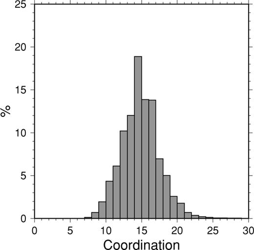
The distribution of node coordination for the final three-dimensional (3-D) node configuration.

Open in new tabDownload slide

The 3-D convergence of the system took 38 iterations to converge fully, i.e. when the Delauney configuration of tetrahedra was stable and the conjugate gradient algorithm gave no further decrease of the energy E (Fig. 10). The CPU times needed were very acceptable (less than 1 min per iteration on a Mac PowerBook G4).

Figure 10

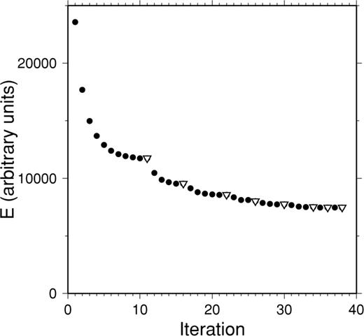
Convergence of the three-dimensional (3-D) optimization. The circles denote the convergence of the conjugate gradient optimization without changing the Delauney configuration of node connections. The inverted triangles denote the energy of the spring system just before a new Delauney triangulation is computed. The convergence was stopped when no model nodes swapped partners in the triangulation.

Open in new tabDownload slide

In the final configuration, the standard deviation has been reduced to 0.19 and 0.22 < ξ < 2.16, with an average of 1.05 (Fig. 11). The slight bias shown by the average larger than 1 indicates we did not seed the model with enough nodes. The spread of ξ by a factor of approximately 20 per cent with respect to the ideal is acceptable, certainly in view of the fact that the interpolation is effected within tetrahedra, involving four node spacings. Note that even in an Earth with uniform resolution lengths ℓ_ij=L, it would be impossible to construct a parametrization consisting of tetrahedra with facets of length exactly equal to L.

Figure 11

The distribution of ξ= | r_i−r_j|/ℓ_ij for the three-dimensional (3-D) optimized grid before and after optimization.

Open in new tabDownload slide

5 Interpolation

Because tomographic equations are integral equations and insensitive to small detail in the function describing the model, linear interpolation between the four vertices of a tetrahedron will often be sufficient (see also Constable et al. 1993). This is easily accomplished using the concept of barycentric coordinates (e.g. Montelli 2003). Let the four vertices of a tetrahedron be given by points located at r₁, r₂, r₃ and r₄. An arbitrary location in can be written as

14

which defines the barycentric coordinates h_i. To make the h_i unique, we must normalize them:

15

Eq. (14) shows that the barycentric coordinates themselves are the appropriate weights to use in a linear interpolation scheme: if r is at vertex k, all h_i equal zero except h_k= 1 and it is easy to see that the h_i on a facet between a pair of vertices are only dependent on those two vertices, which guarantees continuity of the interpolated field between two adjacent tetrahedra that share that facet. We may therefore solve the three equations in eq. (14) and the condition (15) for the h_i (r) as a function of r. By summing over the contributions of the four vertices of the tetrahedron ▵(r) enclosing r, the seismic model value m(r) can be interpolated:

16

The correspondence with eq. (2) is now obvious. To find the tetrahedron that encloses a location r, we have found the 3-D extension of the walking triangle algorithm of Sambridge et al. (1995) most effective.

In case a smoother interpolation is needed, higher order polynomial interpolations may be used but these generally require knowledge of the gradients and Hessians at the vertices, and have the drawback of substantial computational complexity (Alfeld 1984; Michelini 1995; Awanou & Lai 2002). Braun & Sambridge (1995) developed a natural neighbour interpolation scheme that is simple, but with discontinuous derivatives at facets.

6 Discussion

We have presented a practical method that yields a spatial distribution of nodes or interpolation supports in the Earth that closely matches an imposed pattern of node spacings. It is important to generate a distribution that has a local node density that is close to the desired density. A conjugate gradient algorithm is then sufficient to optimize the node locations.

The method allows for an analytical expression of gradients, in contrast to reparametrization schemes that optimize ratios between singular values of the system of tomographic equations (Curtis & Snieder 1997), or that attempt to match gradients in the solution (Sambridge & Faletič 2003). It is also much less aggressive than the latter scheme, which works by subdividing tetrahedra, generating many more unknowns in the problem with every adaptation.

So far, we have not addressed how to estimate the resolving lengths ℓ_ij for a given tomographic problem. For a linear problem of the form Am=d with a generalized inverse A⁻, the solution estimate is given by m_e=A⁻d=A⁻Am=Rm, where R is the resolution matrix (Wiggins 1972). If R can be explicitly computed, the width of the region along the ith row where non-diagonal terms are significantly different from zero defines the resolution length near node i. Note that this definition differs from the unbiased resolution estimate defined by Backus & Gilbert (1968), because the rows of R do not sum to one, so that m_ei is not a true average of the model around node i. Nolet (1985) gives an algorithm to compute true averaging kernels for resolution estimation, though at the expense of a significant increase in computation time.

Unfortunately, 3-D tomography problems are usually so large that the generalized inverse cannot explicitly be computed and the best we can do is try to estimate the true resolution. Vasco et al. (2003) show that the ray density provides a first-order estimate of local resolution for an extensive set of body waves traversing the mantle and core of the Earth, except in the region of the Pacific where significant trade-offs occur long the dominant ray direction. A similar conclusion was obtained by Simons et al. (2002) for surface wave tomography. The next best estimate is described by Nolet et al. (1999), who define the generalized inverse by a one-step backprojection. It provides a first-order correction for the effects of dominant ray directions. This, however, comes at the expense of a significant increase in computation time. Even more CPU expensive, but superior from the point of view of accuracy, is the Lanczos scheme with frequent re-orthogonalization described by Vasco et al. (2003) and the parallel implementation of Cholesky factorization by Boschi (2003).

The most practical approach may be offered by sensitivity tests. Such tests, if a synthetic model of delta-like velocity anomalies is used to generate a synthetic data set that is subsequently inverted using an iterative matrix solver such as LSQR, provide a sparse sampling of the resolution. We suggest that this sparse sampling is used to calibrate the ray density map, or that one simply interpolates between the known resolution. This may be the best compromise between computation time and estimate accuracy. The sensitivity test should be done on an oversampled model and its results can then be used to reparametrize the model along the lines described in this paper.

A user-friendly version of the optimization software is in preparation and will be made available through the IRIS Data Management Center (http://www.iris.washington.edu/manuals). Until then, a research version can be obtained on request from the authors ([email protected]).

Acknowledgments

This research was supported through NSF-EAR0345996. We are grateful to Malcolm Sambridge for giving us his walking algorithm software as well as for his generous advice. His review and that of an anonymous referee did help us to improve the paper.

References