A non-parametric hazard model to characterize the spatio-temporal occurrence of large earthquakes; an application to the Italian catalogue

Summary

1 Introduction

The statistical modelling of the spatio-temporal distribution of earthquakes is an indispensable tool for extracting information from the available data on the physics of the earthquake occurrence process, and for making reliable earthquake forecasts. As regards theoretical aspects, a satisfactory modelling might allow testing of, at least in principle, a variety of hypotheses, such as the presence of any regularity in time, and the influence of different tectonics/physics factors that regulate the spatial occurrence of earthquakes. At the same time, reliable earthquake forecasting has undoubtedly a huge social impact because it may mitigate the seismic risk.

Many papers in the past were focused on studying the distribution of earthquakes (e.g. Vere-Jones 1970; Shimazaki & Nakata 1980; Nishenko 1985; Boschi 1995; Ellsworth 1998; Ogata 1998; Kagan & Jackson 2000; Stock & Smith 2002; Posadas 2002, and many other references therein), but the results obtained seem, in some cases, contradictory. Apparently, the factors that contribute mainly to such differences are the magnitude threshold and the spatial scale investigated. As a matter of fact, a spatio-temporal clustering for mainshock-aftershock sequences is widely accepted, but it has been suggested that the statistical distribution of large earthquakes, overall in well defined seismic regions or on single faults, might be different (e.g. Shimazaki & Nakata 1980; McCann 1979; Nishenko 1985; Papazachos & Papadimitriou 1997; Ellsworth 1998).

Very often, the distribution of large earthquakes is studied only in the temporal domain, by selecting small seismic areas where the hypothesis of spatially homogeneous sampling probably holds. Unfortunately, these small areas do not usually contain a sufficient number of earthquakes to test adequately any hypothesis and model (cf.Jackson & Kagan 1993). For this reason, quite different distributions, such as Poisson (e.g. Kagan & Jackson 1994), Poisson generalized (e.g. Kagan 1991), Brownian Passage Time (Ellsworth 1998), Weibull (Nishenko 1985), lognormal (e.g. Nishenko & Buland 1987; Michael & Jones 1998) distributions, or competitive models, such as general seismic gap hypothesis (McCann 1979), time-predictable model (Shimazaki & Nakata 1980; Papazachos 1992), clustering of earthquakes (e.g. Kagan & Jackson 2000), are still commonly used in hazard studies.

The present scarce knowledge about this issue is well highlighted by the fact that, in some cases, these antithetical models are simultaneously used (e.g. Working Group on California Earthquake Probability 1999). Remarkably, the differences between these models are not only of a statistical nature, but they imply opposite physical mechanisms for earthquake occurrence. In summary, the rationale under the choice of any model is very often based only on theoretical assumption or on a personal subjective belief.

The problem in defining the distribution of earthquakes is further complicated by the ambiguous definition of terms such as mainshock-aftershock, and ‘large’ earthquake. The latter, in particular, seems strongly related to the tectonic region considered. In Italy, for instance, earthquakes with M≥ 5.5 are usually defined ‘large’ and they are considered independent of each other (e.g. Boschi 1995, see also below), while in the Pacific Ring many of such events are clear aftershocks of larger events (e.g. Kagan & Jackson 2000).

The aim of this paper is to provide a new method of analysis to characterize the spatio-temporal distribution of large earthquakes. We use a multivariate non-parametric hazard model that presents several, important theoretical and technical advantages compared to more traditional approaches. With regard to the temporal domain, the method allows finding of a base-line empirical hazard function, whose trend provides very useful information on the physics of the process that generates earthquakes.

The hazard function specifies the instantaneous rate of occurrence at a time T=t, conditional upon survival to time t. As the hazard function describes unequivocally the statistical distribution of the events, its empirical trend provides an immediate tool to rule out some of the distributions mentioned above. Moreover, it gives an immediate answer to the famous Davis et al.’s question (1989)

‘Can it be that the longer it has been since the last earthquake, the longer time till the next?’

The answer to this question depends essentially on the statistical distribution of the inter-event times, as also shown by Sornette & Knopoff (1997). An increasing trend of the hazard function would provide an answer ‘no’ to such question. On the other hand, a negative trend would lead to an answer ‘yes’. In other words, a monotonic increasing trend would stand for an increase in the probability of occurrence with the time elapsed since the last event. This case would support, in general, the seismic gap hypothesis (McCann 1979; Nishenko 1985), as well as any general model based on the ‘characteristic earthquake’ with almost constant recurrence times (e.g. Schwartz & Coppersmith 1984). On the other hand, a monotonic decreasing trend of the hazard function would stand for a ‘clustered’ sequence, where the probability of occurrence decreases with the time elapsed since the last large event. A constant hazard function characterizes the Poisson process; in such case the conditional probability to have an earthquake in a fixed time interval is ‘time independent’, i.e. it is independent from the time elapsed since the last event.

For what concerns the spatial domain, the method proposed in this paper presents many significant differences compared to techniques used in previous works (e.g. Kagan & Jackson 2000; Stock & Smith 2002). In particular, the latter account for the spatial variability simply by filtering the epicentre locations through suitable kernel functions. This strategy implies that the spatial inhomogeneity is mainly explained by the different rate of occurrence of the earthquakes, without considering the influence of the different tectonics/physics parameters. On the contrary, the technique described here may account for any tectonics/physics factor that can potentially influence the spatial distribution of the events, and test statistically their relative importance. This is accomplished by attaching at each inter-event time between earthquakes a vector of covariates which describes the seismic events as well as the spatial/tectonic characteristics of the region where the earthquakes occurred.

The technique is robust because it considers all of the spatially inhomogeneous data simultaneously to build the statistical model; moreover, it allows use of the censoring times that carry out a certain amount of information on the process of earthquake occurrence and that are not usually considered in more traditional approaches. At the same time, the technique is very flexible, being based on a small number of mild assumptions. After having delineated the details of the technique, we apply it to the seismic catalogue of strong earthquakes occurred in Italy in the last centuries (Working Groups on CPTI, 1999, and CSTI, 2001). In particular, we focus our attention on (i) identifying the trend of the hazard function, (ii) checking the influence of rates of occurrence and magnitudes as responsible for the spatio-temporal variability, and (iii) estimating the probabilities of occurrence for future large earthquakes in Italy.

2 The Statistical Model

Here we model the spatio-temporal occurrence of earthquakes through a non-parametric multidimensional fit of the hazard function. In particular, we use the proportional hazard model described by Cox (1972) and Kalbfleisch & Prentice (1980).

As there is a biunivocal correspondence between the hazard function and either the probability density function or the cumulative and survivor functions (e.g. Kalbfleisch 1985), the hazard function defines unambiguously the statistical distribution of the inter-event times. Nevertheless, the hazard function is often preferable because a simple analysis of its trend can provide useful insights on the physics of the process. For example, some of the most used statistical distributions (i.e. the Weibull distribution) were built by imposing a parametric form (a power law) for the hazard function.

Basically, the model deals with two kinds of random variable (RV), namely the inter-event time (IET) between two consecutive earthquakes, and the censoring time (CT), i.e. the time interval between the present time and the last earthquake occurred. At each one of these RVs a vector of explanatory variables (from now on covariates) has been attached that carries out any kind of information relative to the IET or CT considered. In particular, in the analysis of a seismic catalogue, the vector of covariates can contain any spatial/tectonic information on the subregion where the IETs and/or CT are sampled.

The proportional hazard model (Cox 1972; Kalbfleisch & Prentice 1980) for a generic time x^★ since the last event can be written as

1

where z is the vector of covariates, β is a vector of coefficients, and λ₀(x^★) is an arbitrary and unspecified base-line hazard function. The dimension of the vectors z and β is M, which represents the number of (quantitative and qualitative) covariates considered in the analysis. The survivor function (S) and pdf ( f) for such a model are

2

and

3

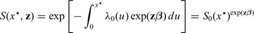
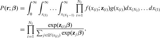
Note that the covariates act multiplicatively on the hazard function and that z does not depend on time (eq. 1). This means that the ‘form’ of the base-line λ₀(·) is always the same apart from a multiplicative factor that depends on the covariates. From a physical point of view, this means that the mechanism of earthquake occurrence (described by the function λ₀(·)) is the same for different areas; only the parameters of the system can vary (i.e. exp(zβ)). The model is non-parametric because it does not assume any specific form for the base-line hazard function, therefore it is more flexible compared to the traditional parametric approaches. In practice, it means that we do not impose any a priori assumption on the mechanism of the earthquake occurrence process, but the most likely probabilistic model is suggested by the empirical data.

The main problem here is to estimate β and the non-parametric form of λ₀(·) in eq. (1). These quantities have a great importance. The coefficients contained in vector β give the relative importance of each covariate considered. The form of λ₀(·) gives important insights on the physics of the process.

2.1 Estimation of β

Let us suppose N inter-event times x_i (i= 1, …, N) and the corresponding covariates z_i. For the sake of simplicity, at this first stage we do not consider the CTs and possible ties in x_i. Let us define two additional vectors, o(x_i) and r(x_i)

4

5

where x_(i) are the IETs ordered in increasing order.

We can image a number of transformations of the variable x through strictly increasing a differentiable transformation of (0, ∞) onto (0, ∞). Since λ₀(·) is completely unknown, the inference problem about β is only based on the vector r(·), because it is the only one that is always invariant under the transformations done on x. In technical terms we can say that r(·) is sufficient for the estimation of β in the absence of knowledge of λ₀(·). In such case, the likelihood is proportional to (see Kalbfleisch & Prentice 1980)

6

where f(·) is the pdf (see eq. 3), and Ω(x_(i)) is the set of labels attached to the IETs with length ≥x_(i), that is Ω(x_(i)) ={(i), (i+ 1), … (N)}.

In most practical cases, such as in the hazard studies, it is very important to take also into account CTs which often represent a significant part of the available data. For instance, it is very common to have very few earthquakes inside each seismic area, therefore the only CT available for that area is usually a relevant percentage of the data. To properly handle CTs we need to introduce some modifications to eq. (6). The greatest problem in dealing with CTs is that their statistical distribution is almost certainly different from the distribution of the IETs (e.g. Kalbfleisch & Prentice 1980) and it is very difficult to figure out. Here, as well as in most of the scientific literature on this issue, a random mechanism is assumed for the censoring. In practice, this implies that the end of the seismic catalogue is independent of the time of occurrence of the last earthquakes in each zone. From a statistical point of view, this also means that the CTs are RVs stochastically independent of each other and of the IETs. Note that this hypothesis seems very reasonable for earthquake catalogues.

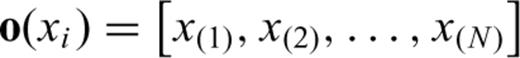
Let us consider N₁ IET, x₍₁₎, …, x, with corresponding covariates z₍₁₎, …, z, and , of which n_i are censored in the i-th interval [x_(i), x_(i+1)), i.e. , and with covariates z_{i 1}, …, z. The CTs contain only partial information on the rank vector r(·), because the ordering vector including the CTs is not necessarily the ‘true’ ordering that we would have if we waited for the occurrence of the earthquakes. In this case, the contribution of the CTs in the time =

7

Therefore eq. (6) can be rewritten as

8

where Ω′(x_(i)) is the set of labels attached to the IETs and CTs with length ≥x_(i), i.e. Ω′(x_(i)) ={[(j), j1, …, jn_j], j=i, …, N₁}.

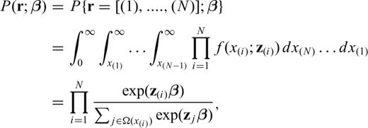
In both cases, eqs (6) and (8) are the product of single terms, each one representing the rate between the hazard function of the i-th IET, and the sum of the hazard functions relative to the IETs and CTs ≥x_(i). In practice, we can consider each IET and CT as labelled objects with a weight exp(zβ). In this picture eq. (8) calculates the probability of observing a particular sequence of labels relative only to the IETs. Note that eq. (8) is not the probability to get the observed IETs and CTs in the censored experiment. This probability would depend on the (unknown) censoring mechanism and also on the form of λ₀(·). Eq. (8) is the probability that, in the underlying uncensored version of the experiment, the event consisting of the IETs and CTs observed would occur.

Finally, let us consider the possibility of having some ties in the data. This can occur, for instance, when the measurement errors lead to some kind of binning of the IETs (e.g. for palaeoseismic data). For this purpose we use the same strategy used to incorporate the CTs. Suppose d_i IETs with length x_(i) (i= 1, …, N₁), where x₍₁₎, x₍₂₎, …, x, and (no censoring). In this case we still have partial information on the rank vector, as for the CTs above. Although the ranks of IETs with length x_(i) are known to be less than those with length x_(j) (i < j), the arrangement of the ranks of the d_i IETs is otherwise unknown. As before, it is hardly conceivable to take into account all the possible dispositions of the ranks. Peto (1972) and Breslow (1974) have shown that if the number of ties d_i is small compared to the number of objects contained in the set Ω (see eq. 6), the likelihood can be written as

9

where s_i is the sum of the covariates of the IETs with length x_(i).

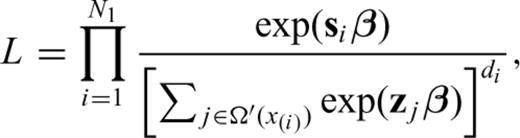
The Maximum Likelihood Estimation (MLE) can be obtained as a solution of the system of equations

10

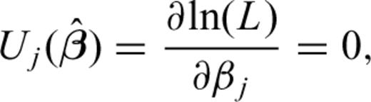
where U_j is the score vector (e.g. Kalbfleisch 1985). Even though only partial checks have been performed on this field until now, it has been suggested that only mild conditions on the covariates and censoring are required to ensure the asymptotic normality of . Some numerical investigations, for instance, have shown that the asymptotic normality is a good approximation for data sets with no ties and less than 10 data (Kalbfleisch & Prentice 1980). In this case has a pdf , where I_jk is the information matrix (Kalbfleisch 1985).

11

This allows a direct test to check the relative importance of the factors included in the covariate vector. As a matter of fact, the question of the adequacy with which the asymptotic form of the distribution approximates the actual sampling distribution must be kept in mind in any practical applications. In cases where equivocal results arise, it might be wise to perform some numerical check for the sampling distribution of .

2.2 Estimation of the base-line function

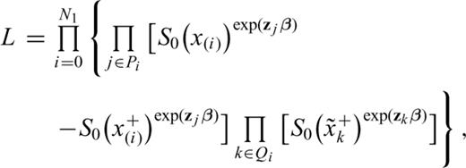
Now the problem is to estimate the shape of the base-line function λ₀(·). As a first step we focus our attention on eq. (2) and estimate S₀(·). As before, let x₍₁₎, x₍₂₎, …, x be the IETs, let P_i be the set of labels associated with the IETs with length x_(i), and Q_i the set of labels associated with the CTs censored in [x_(i), x_(i+1)) (i= 0, …, N₁), where x₍₀₎= 0 and x=∞. 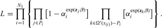The CTs in the interval [x_(i), x_(i+1)) are where j ranges over Q_i. The contribution to the likelihood of an IET with length x_(i) and covariates z is, under ‘independent’ censorship,

12

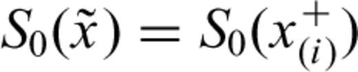
where S₀(x⁺_(i)) = limS₀(x_(i)+δ). The contribution of a CT is

13

Therefore, the likelihood can be written as

14

where P₀ is empty. It is clear that L is maximized by taking for 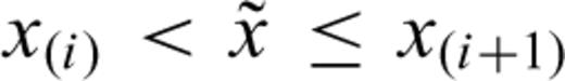and allowing probability mass to fall only at the observed IETs x_(i).

The form of the base-line function is completely empirical, therefore it has a discrete form. The survivor function at a generic time x^★ since the last event for a discrete process with CTs is (Kaplan & Meier 1958)

15

where λ_j=P(X=x_j|X≥x_j). Note that eq. (15) is the discrete version of eq. (2). These observations lead to the consideration of a discrete model with hazard contribution λ_j at x_(j) (j= 1, …, N₁). Thus we take

16

where α₀= 1. Substituting eqs (2) and (15) in eq. (14), and rearranging the terms we obtain

17

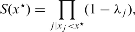
The estimation of the survivor function can be carried out by joint estimation of the α_i and β in eq. (17). More simply, we can take as estimated previously and then maximize the logarithm of eq. (17) with respect to α_i. In this case we obtain

18

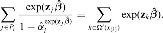
If we do not have ties, eq. (18) can be directly solved for , otherwise an iterative solution is required. A suitable initial value for such iteration is

19

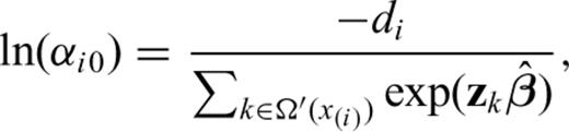
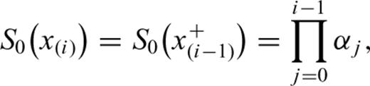
obtained by approximating . The MLE of the base-line survivor function for a generic time x^★ since the last earthquake is therefore

20

which is a step function. The equation of the proportional model for a generic time x^★ and covariates z^★ is

21

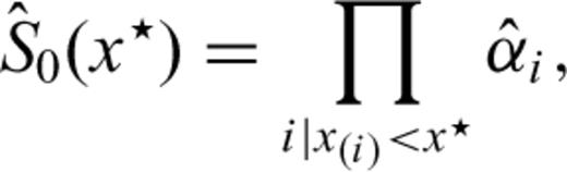
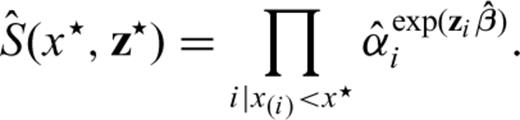
As mentioned before, the trend of the function λ₀(x) has an important theoretical and practical meaning. A simple way to show such a trend is through the comparison of the empirical survivor function and the survivor function for the Poisson process. Let us consider the transformation

22

that makes the RV u(x) asymptotically normally distributed (e.g. Kalbfleisch & Prentice 1980). The transformation (22) applied to the survivor function of the Poisson process gives u_P(x) = lnλ+ ln(x). Therefore, a plot of the residuals

23

versus x shows the departures of the empirical survivor function from a theoretical Poisson distribution. By looking at eq. (22) and to the relation between survivor and hazard function, it is easy to show that the trend of ɛ(x) has a behaviour comparable to the trend of λ₀(x).

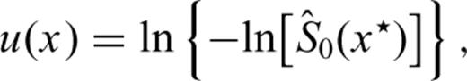
3 Checking the Model

A basic step of each kind of modelling is the statistical validation of the model. It is well known by now that the check of any model, regardless of its nature, should be performed on an independent data set, i.e. on data that have not been considered at any step of the modelling. For time sequences, a certain independent data set is given by future events. In any case, a preliminary check can be done by dividing the available data set in two, one used to set up the model (the learning phase), and the other to check the model (the validation phase). This approach provides a necessary condition for the validity of the model. In other words, if the model does not fit the available data we can disregard it. On the contrary, if the model fits well we cannot rule out the possibility of an overfitting due to unconscious suitable choices. This chance may be drastically reduced by using a model with a number of parameters much lower than the independent observations used. In any case, as mentioned before, the real capability of the model to describe the process can be obtained only in real forward analysis.

As regards the model described in the previous section, the goodness-of-fit can be empirically checked by using independent data of the validation phase. Each IET (x) of this data set is transformed through the equation

24

where

25

(see eqs 2 and 19–20) and are estimated by the data of the learning phase. If the model is appropriate, the residuals should be similar to a sample drawn by an exponential distribution with λ= 1 (Kalbfleisch & Prentice 1980, see also Ogata, 1988). Therefore, a comparison of the cumulative of the residuals with a theoretical exponential curve provides a goodness-of-fit test of the model. The comparison can be statistically checked through a one-sample Kolmogorov-Smirnov test (e.g. Gibbons 1971).

4 Application to the Italian Territory

Here, for the sake of example, we apply the proportional hazard model to the Italian seismicity. We use the parametric seismic catalogue published by the Working Group on CPTI (1999) integrated with more recent data (since 1980) coming from the Working Group on CSTI (2001) and from the Bulletin of the Istituto Nazionale di Geofisica e Vulcanologia (INGV). In order to have a complete set of events we consider the earthquakes with M≥ 5.5 since 1600 (see Fig. 1). The threshold magnitude has been chosen taking into account practical aspects. In fact, M= 5.5 generally represents a threshold value for which the earthquakes in the Italian territory are considered ‘dangerous’ due to the high number of historical buildings. Previous papers assume that similar events are almost independent of each other (e.g. Boschi et al. 1995). This assumption would seem corroborated by the analysis of the autocorrelation and of the goodness-of-fit with a Poisson distribution of the IETs calculated for the whole Italian catalogue (see Figs 2a–b). In particular, the two null hypotheses, of no autocorrelation and no departures from a Poisson process, are not rejected at a 0.05 significance level.

Figure 1

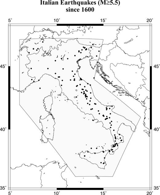
Map of the earthquakes with M≥ 5.5 since 1600 in Italy.

Open in new tabDownload slide

Figure 2

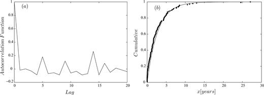
(a) Plot of the empirical autocorrelation function of the IETs calculated for the whole Italian catalogue. (b) Empirical cumulative distribution of the IETs calculated for the whole Italian catalogue.

Open in new tabDownload slide

The results obtained from the analysis of the whole catalogue may be strongly biased because the events can be hardly considered as an homogeneous sample. The Italian territory presents a strong and complex spatial variability due to the presence of different tectonic domains. In order to account for the inhomogeneities in the spatial distribution of the events, we consider a 13 × 13 grid between the latitudes 36–48°N, and longitudes 5–20°E (see Fig. 1). Each node of the grid is the centre of a circle. In order to cover the whole area the radius R of the circle is set about , where D is the distance between the nodes. For such grid, D≈ 100 km and R= 70 km.

In a following step, we select the circles that contain at least 3 earthquakes; for each one of these circles we calculate the IETs among the earthquakes inside the circle, one CT relative to the time elapsed since the last event, and a vector of covariates z attached to each RV that may accommodate the characteristics of the earthquakes as well as the spatial/tectonic characteristics of the circle considered. Here, for each RV we consider a 2-D vector z composed by the rate of occurrence, i.e. the total number of clusters occurred inside the circle divided by 403 yr (1600–2002), and by the magnitude of the event from which we calculate the IET and the CT. The latter might be relevant in case the earthquakes occur following any general model where the probability to have another large earthquake in a given time interval depends on the magnitude of the last event. Some examples are the ‘time predictable’ model (Shimazaki & Nakata 1980; Papazachos & Papadimitriou 1997), and the stochastic models (mainly based on the Gutenberg-Richter and a general Omori law) that describe the number of triggered events as a function of the magnitude of the triggering predecessor (e.g. Ogata 1988; Kagan & Jackson 2000).

By using the data of the Italian catalogue (see Fig. 1) and eqs (10)–(11), we obtain β₁= 55 ± 8 and β₂= 0.2 ± 0.2. The first coefficient, β₁, is the first component of the vector , i.e. the coefficient that is linked to the rate of occurrence. The coefficient β₂, instead, is linked to the magnitude of the event from which the IET is calculated. As it appears clear, β₂ is not significantly different from zero, thus the magnitude of the events is not relevant for the distribution of the IETs. On the contrary, β₁ is positive and significantly different from zero.

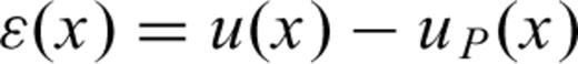
In Fig. 3 we report the empirical survivor function of eq. (20). Compared to the Poisson distribution, such empirical survival function has a greater number of small IETs. This departure is shown in Fig. 4, where the plot of the residuals ɛ(x) (see eq. 23) is reported. As mentioned above, the trend of ɛ(x) is comparable to the trend of λ₀(x). The decreasing trend means that the earthquakes tend to be more clustered that in a simple Poisson process. The negative trend lasts for few years after the event, then the trend becomes almost flat as expected for a Poisson process. The presence of a significant departure from the Poisson model implies that the statistical distribution is time dependent, i.e. the probabilities of occurrence depend on the time elapsed since the last event. Note that there is no significant evidence of a positive trend.

Figure 3

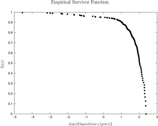
Empirical base-line survival function (eq. 20) for the Italian seismicity.

Open in new tabDownload slide

Figure 4

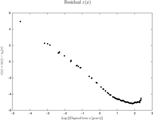
Plot of the residuals ɛ(x) (eq. 23) as a function of the time elapsed since the last event.

Open in new tabDownload slide

In Figs 5(a)–(b) we report the graphs representing the goodness-of-fit for the learning and validation data sets (see eq. 24). In particular, we use the time interval 1600–1950 for the learning phase (124 earthquakes), to set up the model. The time interval 1951–2002, instead, is used for the validation phase (21 earthquakes), to verify the model with an independent data set. The figures clearly show that the model fits the data very well, both in the learning and validation data sets. The goodness-of-fit is evaluated quantitatively through a one-sample Kolmogorov-Smirnov test (e.g. Gibbons 1971). The significance levels at which the null hypothesis of equal distributions is rejected are reported in the figures. In both cases, they are >0.10.

Figure 5

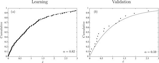
(a) Empirical (dotted line) and theoretical (solid line) cumulative functions for the learning data set. The parameter α is the significance level at which the null hypothesis (Poisson hypothesis) can be rejected (see text for more details). (b) The same as for (a), but relative to the validation data set.

Open in new tabDownload slide

In the next step, we calculate, from the empirical survival function of eq. (21), a map of the probability of occurrence for the future large earthquakes. The conditional probability to have an earthquake in the next τ years, given a time t since the last event, can be approximated by

26

where z is the vector of covariates relative to the IET (t, t+τ] of the circle considered. In Figs 6(a)–(b), we report the map of the probability of occurrence for an earthquake of M≥ 5.5 in the next one (τ= 1) and ten (τ= 10) yr in Italy. We identify as the most dangerous regions, a large part of the Northern-Central Appennines, and Central-Southern part of the Calabria; other smaller maxima of probability are located around Garda lake, in Friuli, and in part of Puglia-Basilicata and Sicilia regions.

Figure 6

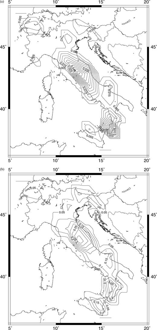
(a) Map of the probability of occurrence for the next large earthquake in Italy calculated for τ= 1 yr (eq. 26). (b) The same as for (a), but relative to τ= 10 yr.

Open in new tabDownload slide

As a final step, we evaluate the forecasting ability of the model through a retrospective forward modelling. For this purpose, we calculate the probabilities of the regions where earthquakes with M≥ 5.5 have occurred since 1950. The model can be considered ‘forward’ because we calibrate it only by using data available immediately before each earthquake. In order to make it easier to check the forecasting capability of the model, we bin the probabilities in four categories: ‘HIGH’, ‘MEDIUM’, ‘LOW’, and ‘NEGLIGIBLE’. The categories are assigned by ranking the probabilities of each circle. A rank equal to i means that there are i− 1 regions with higher probabilities. Then, we attach the category ‘HIGH’ to the regions that have a probability rank below the median, the category ‘MEDIUM’ for the regions above the median, the category ‘LOW’ for the regions with less than three seismic events (for which we do not calculate the probability), and the category ‘NEGLIGIBLE’ for the regions where no historical earthquakes occurred. In total, 46 circles experienced historical earthquakes, and 29 have 3 or more events. The results of the ‘forward’ analysis are reported in Table 1. In the period 1951–2002 (the validation data set), 16 out of 21 events occurred inside the 29 circles that experienced three or more events in the past: 13 inside circles with HIGH probability, and three inside circles with MEDIUM probability. Remarkably, 10 out of 21 occurred in the five circles with the highest probabilities.

1

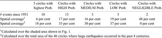
Results of the retrospective forward simulation. The number of forecast earthquakes for each kind of binned probability circle (see text) are reported, together with two different type of spatial coverage.

Open in new tabDownload slide

We have positively checked the stability of the results by using the seismic catalogue in a shorter period (since 1700), and two different grids, a 9 × 9 (D≈ 140 km and R= 100 km) and a 19 × 19 (D≈ 70 km and R= 50 km).

5 Discussion and Concluding Remarks

The main goal of the present paper was to propose a new non-parametric and multivariate method to characterize the spatio-temporal distribution of large earthquakes. The method has several advantages compared to more traditional approaches. It allows accounting for many different factors that can potentially influence the spatio-temporal distribution of earthquakes, and it provides a direct tool to test the relative importance of these factors. Moreover, the method is almost completely non-parametric. Compared to other stochastic models proposed in the past (i.e. Ogata 1988; Kagan & Jackson 2000) the method does not assume any a priori stochastic model for the time behaviour. Therefore, the empirical time behaviour found by the model (see, for instance, Fig. 3) furnishes a direct and formal check of the reliability of antithetic models of earthquake process generation, such as the ones based on seismic gap, Poisson, and cluster hypotheses.

The technique has been then applied to the Italian historical large earthquakes. The first result obtained is that large earthquakes (M≥ 5.5) in Italy tend to cluster in time and space. The time length of the cluster may reach a few years; after this time the distribution of the earthquakes becomes a Poisson distribution. Note that the time clustering seems to be longer than what was expected for a typical aftershock sequence (e.g. Gasperini & Mulargia 1989; Console & Murru 2001, see also Helmstetter & Sornette 2003). Remarkably, we do not find any evidence of increasing hazard function. This result seems to rule out any statistical distribution characterized by an almost constant recurrence time, as the Weibull with β > 1 (Nishenko 1985), the lognormal (e.g. Nishenko & Buland 1987; Michael & Jones 1998), the Brownian Passage Time (Ellsworth 1998), and all the other statistical distributions with an increasing hazard function. This is also in antithesis to the seismic gap model (McCann 1979) which assumes that recent earthquakes deter future ones. This result is instead in agreement to what was found through different techniques by Ogata (1998), Kagan & Jackson (2000), and Rong & Jackson (2002) in other seismic regions.

With regard to the spatial dimension of the cluster, this is in part imposed by the choice of R. This choice was mainly driven by two antithetical practical aspects; the need to have the largest number of circles having three or more events, but with the surface as small as possible. The last requirement is the necessity to have almost tectonically homogeneous circles, and to make earthquake forecasting useful for hazard studies. In spite of this, we have observed comparable time clustering also by using different grids (see above), we argue that such time behaviour may depend on the spatial scale adopted, since it is hardly conceivable that the same time clustering holds at the two extremes of the spatial domain, i.e. for a single fault and for the whole earth. In particular, since the average of the IETs for each circle is definitely lower than the time expected to reload a fault through tectonics (in Italy, about 10³ yr; see, e.g. Pantosti 1993), we speculate that the long-term clustering found at the spatial scale defined by the dimension of the circles might be the result of the interaction among a probably high number of seismogenic faults, some of them close to the rupture. In this perspective, at such a spatio-temporal scale, the interaction between faults seems to be more relevant for earthquake forecasting purposes, than the behaviour of a single seismogenic fault.

Another interesting result obtained is that the length of the inter-event times is independent of the magnitude of the earthquakes. In other words, the magnitude of the last event does not modify the probability to have another large event. From a physical point of view, this means that there is no evidence in favour of some kind of ‘time predictable’ model (Shimazaki & Nakata 1980; Papazachos & Papadimitriou 1997). This result is also in contradiction to the models characterized by a time behaviour that depends somehow on the magnitude of the earthquakes (e.g. Ogata 1988; Kagan & Jackson 2000). Remarkably, this might lead to suggest that the Gutenberg-Richter law does not always hold, at least for large events occurring in small spatio-temporal windows.

The model has been also used to calculate the map of the probability of occurrence for the next large earthquakes in Italy. The same calculation has been made on a validation data set (1951–2002) through a retrospective forward analysis. This has allowed evaluation of the forecasting ability of the model, and to check its statistical reliability. The satisfactory forecasting ability provides further evidence that the earthquakes tend to occur in the regions that experienced many large events in the past (e.g. Kagan & Jackson 1991, 2000), also recently (e.g. Kagan & Jackson 1999). As stated before, this is in contradiction with any sort of seismic gap hypothesis.

As a final consideration, we remark that the map of the probability of occurrence for the next large earthquakes reported here should be regarded only as a first attempt in this direction. Here, in fact, we have only considered information coming from a seismic catalogue disregarding all the geological/tectonics variations that characterize the Italian territory. A reliable regionalization, the state of stress, the number and kind of tectonic structures, the modelling of possible interactions among different regions, are only some of the parameters to add to the vector z (see, i.e. eq. 1) that might improve significantly the maps reported in Figs 6(a)–(b). Future works will be addressed on this direction.

Acknowledgments

We would thank Rodolfo Console for helpful comments on the original version of the paper. This work was financially supported by a GNDT project.

References