Empirical path and station corrections for surface-wave magnitude, M_s, using a global network Free

Summary

1 Introduction

Surface-wave magnitude, M_s, is one of several magnitude scales commonly used in seismology. M_s is of particular interest for two reasons. First, it is perhaps the most useful scale for determining the size of shallow earthquakes. It is believed that the correlation between the M_s and the logarithm of the seismic moment, log₁₀M₀, of a seismic disturbance is higher than for any other magnitude scale (Kanamori 1977; Ekström & Dziewonski 1988). Since M₀ can only be measured directly for large, recent events, M_s can be of use in studies where the energy release of an earthquake is of interest; for example, seismic risk assessments and regional tectonics. Second, the ratio of body-wave magnitude to surface-wave magnitude, m_b: M_s, is one of the most robust methods used in ‘event-screening’, that is, the identification of definite earthquakes in a population of seismic disturbances of unknown origin. Hence the accurate measurement of M_s is vital for monitoring compliance with Comprehensive Nuclear Test Ban Treaty (CTBT).

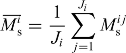
The use of the M_s magnitude scale makes the implicit assumption that the amplitude of a surface-wave at a particular recording station is related directly to the size of the seismic disturbance which generated the wave. When several stations record an M_s for the same event, there is generally some scatter and the network average , is used as the magnitude. Here we discuss the possible causes for the scatter in M_s, and present experiments to calculate empirical path and station corrections for M_s on a global basis using observations from the partially-completed seismological network of the International Monitoring System (IMS) currently being established to monitor compliance with the CTBT. We make use of the surface-wave measurements included in the Reviewed Event Bulletin (REB) of the prototype International Data Centre (pIDC) and the International Data Centre (IDC) during the period 1997 January–2002 December inclusive. The REB is invaluable for such a study since it is the only example of routine measurement of M_s, using an automatic algorithm, from centrally-collected waveforms recorded by a global network of seismometers.

We then discuss the implications of our results, both for event-screening using the m_b: M_s criterion, and the possible relationship between M_s path corrections and Earth structure.

1.1 Surface-wave magnitude, M_s

The first M_s scale, proposed by Gutenberg (1945), is designed to complement the local magnitude scale M_L, and is defined by:

1

where A is half the peak-to-peak amplitude in μm, Δ the epicentral distance in degrees and S_c an optional station correction. The constant 1.818 is required so that M_s can be compared with M_L. Gutenberg intended that M_s would be measured from 20 s surface waves on horizontal-component seismograms.

Since 1945 several M_s scales have been proposed by various workers. Båth (1981) provides an excellent review and Rezapour & Pearce (1998, subsequently referred to as RP98) give a more recent summary. Surface-wave magnitude scales are generally of the form

2

where T is the period of measurement, C is a constant required so that different scales agree, and the distance term, γlog₁₀Δ, corrects for the fall-off of amplitude with distance, γ being a constant. M_s is now generally measured from vertical component Rayleigh waves since these have are more readily available and less noisy than horizontal components. Recently, RP98 produce two new M_s formulae based on complete ISC and NEIC data sets for the years 1978 to 1993 inclusive. The first, following the traditional form of eq. (2) gives:

3

This is in close agreement with the result of Thomas (1978). The second equation of RP98 makes allowance for theoretically derived contributions to the distance term due to dispersion and geometric spreading to give

4

where the term accounts for geometric spreading and the term is intended to account for the effect of dispersion of the Rayleigh wave Airy phase (Ewing 1957, p. 165). The residual distance term can then be related to intrinsic Rayleigh attenuation, Q_R.

1.2 Scatter in M_s

The various scales mentioned above all assume that a global relationship can be used to determine M_s. In practice, there is observable variation in the magnitude measured when more than one station reports M_s for the same seismic disturbance. The accepted practice then is to calculate the network average M_s, M_s. For event i we calculate

5

where M^ij_s is the magnitude of event i measured at station j and J_i is the total number of stations reporting an M_s for event i.

This variation in M^ij_s may be due to one or more of the following.

1.2.1 Path effects

It has been appreciated since the inception of the surface-wave magnitude scale that the M_s of a seismic source can vary from station to station due to differences in Earth structure from path to path (Richter 1958). Gutenberg (1945) notes that M_s values are systematically low for surface-waves which propagate along the edge of the Pacific basin, and gives corrections to his M_s formula for various paths. Båth (1952) in a proposed M_s scale includes a regional correction which he concludes is dependent on the properties of the path between earthquake and recording station. He confirmed the observations made by Gutenberg (1945). Marshall & Basham (1972) propose an M_s scale

6

where B′(Δ) and P(T) are tabulated distance and path-dependent terms. P(T) is intended to account for differences in dispersion from region to region. Following Carpenter & Marshall (1970) they assume that the Rayleigh wave envelope, E(T), can be approximated by

7

for group speed U(T), based on a set of group speed curves for North America, Eurasia, oceanic and mixed continent-ocean paths. For example, at twenty seconds period, they find that ‘mixed’ paths give an M_s reduced by 0.13 magnitude units (mu) relative to the continents, whereas oceanic path M_s is increased by 0.09 mu.

While it is usually assumed that path effects on M_s are mainly due to variations in the group-speed curve, Rayleigh wave amplitudes around 20s are presumably also affected by attenuation, and indeed recent studies at longer periods show large lateral variations in Rayleigh attenuation (Selby & Woodhouse 2000; Billien 2000). However, the average path lengths used for M_s measurements are relatively short, and it may be that large variations in attenuation exist mainly in the asthenosphere (apart from exceptional regions such as mid ocean ridges) and so are too deep to affect 20s Rayleigh waves greatly.

1.2.2 Station terms

Here we use the phrase ‘station term’ to refer to a constant offset in the values of M_s recorded at a particular station, regardless of the location of the seismic disturbance or the path travelled by the surface wave. This is rather different to the usage of the same phrase by other authors such as Thomas (1978) where the station term includes path effects to some extent. Here the station term must be due to the immediate structure at the station or to differences in instrumentation from station to station. That local structure may influence station amplitudes is evident from the variation with station of Rayleigh ellipticity (Sexton 1977; Boore & Toksöz 1969).

Correct estimation of station terms is particularly important when M_s is used for event screening. Station terms would normally be calculated by averaging large numbers of M_s residuals at a particular station. However, these residuals would be based on observation of earthquakes, which have a specific geographic distribution. Hence it is possible that M_s observations at a station may be dominated by measurements from surface waves travelling along similar paths. An explosion could occur at any azimuth and distance from that station and the path travelled by the surface wave from the explosion could be completely different from the paths travelled from earthquakes, so the calculated station term could be inappropriate. Therefore it is essential that path effects on M_s are removed before station terms are calculated, or preferably both should be calculated together.

1.2.3 Radiation pattern

The concept of M_s and other magnitude scales carries the implicit assumption that the size of an earthquake can be determined from the amplitude of a seismic wave without reference to the radiation pattern. Intuitively, however, we would expect that the scatter in M^ij_s about Mⁱ_s would be strongly affected by the radiation pattern. At regional distances (less than about 2000 km from the epicentre) several studies have shown that the amplitude of surface waves around 20s period can be related to the radiation pattern. Bowers (1997) successfully models Rayleigh and Love wave amplitudes to a maximum distance of 12.8° using the radiation pattern predicted from a source mechanism constrained using teleseismic body-wave observations and finds a maximum range of M_s of 1.15 m.u. In a theoretical study, von Seggern (1970) discusses the effect of radiation pattern on magnitude estimates, and demonstrates that magnitudes can be incorrect by more than one magnitude unit due to radiation pattern. von Seggern (1970) shows that theoretical variation in M_s due to radiation pattern is strongly dependent on the type of source mechanism, with 45° dip-slip earthquakes showing very little scatter. As Bowers & McCormack (1997) point out, compressional dip-slip mechanisms predominate in moment-tensor catalogues and presumably also in the Earth, which may limit the effect of radiation pattern on M_s. von Seggern (1970) also points out that m_b:M_s plots show less scatter for known explosions than for earthquakes, although of course some of this scatter will be due to the effect of radiation pattern on m_b, which can be significant (Bowers & Douglas 1998).

Our experience is that for surface waves at periods near 20s path effects usually dominate over radiation pattern at distances Δ > 20°, which is perhaps surprising.

2 Data

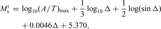
The M_s observations reported in the REB differ from those of other bulletins in that the measurements are made using an automated process on centrally collected waveforms. This means that the method of M_s calculation is invariant, so that systematic variation in residuals, should, subject to a number of provisos, reflect real variations in M_s. Stevens & McLaughlin (2001) describe the method of M_s measurement. Rayleigh waves are detected automatically and associated with known epicentres on the basis of a dispersion test. The algorithm then selects the cycle in the period range 18–22s and the amplitude is measured. M_s is calculated using M^t_S of RP98 (eq. 4 in this paper). Rayleigh waves are reported in the distance range 0° < Δ≤ 100°. The REB reports the instrument-corrected amplitude and period at which the amplitude is measured, together with the magnitude.

2.1 Data editing

Before beginning to interpret the M_s residuals in the bulletin we embark on a thorough process of data editing. This is necessary because we know, as reported in Stevens & McLaughlin (2001), that there have been calibration problems with a number of stations in the IMS network during the period of this study. As an example, Fig. 1 shows data from station CMAR in Thailand. CMAR is one of five long-period arrays in the current IMS network. The top panel of the figure shows log₁₀(A/T) against time. The bottom panel shows the M_s residuals after data editing, with a number of time gaps where data has been excluded. According to Stevens & McLaughlin (2001), all Rayleigh amplitudes in the REB recorded between 1997 April 3 and 1997 June 24 should be considered unreliable. We have therefore omitted all data from this period from the study. Additionally, CMAR underwent a change of instrumentation during the study period which resulted in a period between 1998 October 1 and 1999 May 25 for which the station calibration was incorrect. Stevens & McLaughlin (2001) suggest a correction for CMAR during this time, but after applying the correction we were unhappy with the resulting residuals and so have chosen to omit these data. In fact, the plot of log(A/T) (Fig. 1, top panel) seems to show a trend during this period. The remaining M_s residuals appear to show a definite shift in mean after the change of instrumentation (bottom panel, Fig. 1). We therefore considered these two periods as different stations during the subsequent modelling process. Similar decisions were made for stations ARCES, BGCA, DBIC, ESDC, KBZ, KSAR, NORES, PDAR and TXAR. Table 1 lists the stations used in the study together with the time periods from which data were available at each station. Fig. 2 shows the distribution of these stations. As well as the stations discussed above, two other sets of stations are co-located but cover different time periods (MNV/NVAR and NORES/NOA). Fig. 3 shows the number of observations used at each station. In Fig. 4 we show the distribution of earthquake epicentres used. It can be seen clearly that the small number of stations in the southern hemisphere, together with the restriction of path lengths to less than 100° results in a strong bias in the data set in favour of the northern hemisphere.

Figure 1

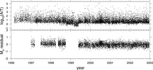
Representation of the data-editing process for station CMAR, Thailand. The top panel shows log₁₀(A/T) plotted against date for the study period. The bottom panel shows the M_s residual (M_s measured at CMAR minus the mean M_s for each event) after unwanted data has been removed.

Open in new tabDownload slide

1

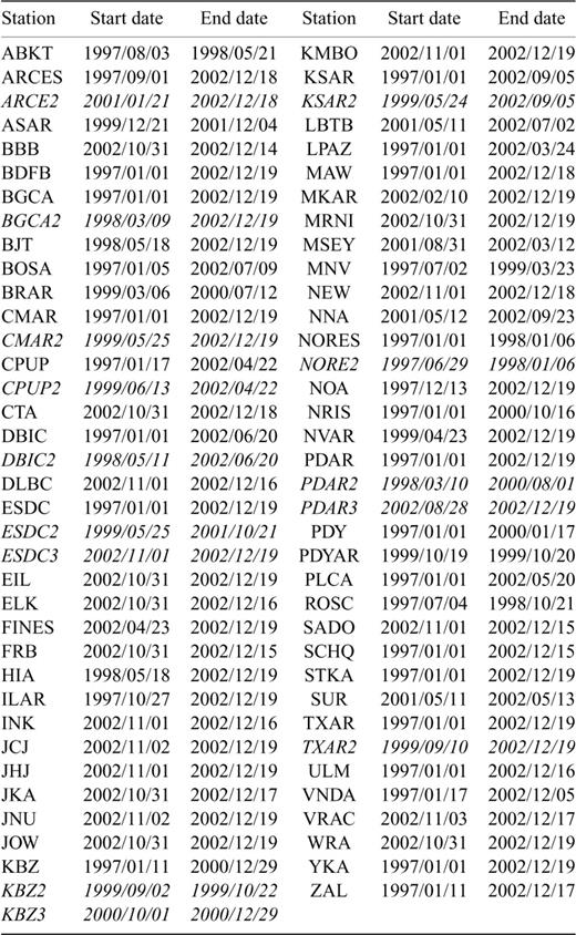
Earliest and latest date for which data are considered for each station utilized in this study. Stations may not be continually operable throughout the period listed. Some stations (including CMAR, ESDC and KSAR) were given alternate names during part of the period; these dates are shown in italics.

Open in new tabDownload slide

Figure 2

Distribution of stations used, which form part of the seismological network of the IMS. Note the co-location of some of the stations.

Open in new tabDownload slide

Figure 3

Number of observations of M_s at each station considered at the beginning of the modelling process. Note that for many stations the number of observations is small.

Open in new tabDownload slide

Figure 4

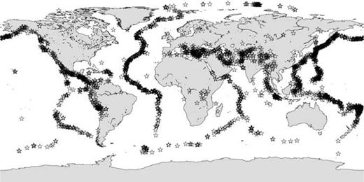
Distribution of epicentres of events used. To be included, there must be at least ten observations of M_s from the event, resulting in a sharp reduction of available events in the southern hemisphere.

Open in new tabDownload slide

In addition to problems with instrument calibration we found a number of discrepancies in the REB where M_s appeared to be calculated from more observations than were listed in the bulletin. We chose to exclude these events from subsequent analysis as the cause of these discrepancies is not immediately apparent.

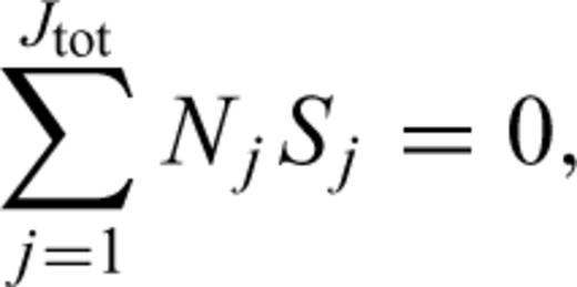
After the data editing process outlined above we then recalculate all the M^ij_s and Mⁱ_sj for the remaining observations. At this point we restrict subsequent analysis to events with J_i≥ 10. This is to ensure that the modelling process begins with a reasonable value for and hence a good estimate of the ‘true’ surface wave magnitude of the event i, .

3 Interpretation

3.1 Observed M_s residuals

Fig. 5 shows the pattern of M_s residuals observed at station ESDC in Spain. The residuals are plotted at the epicentre of the earthquake from which they arise. The size of the symbol is proportional to the size of the residual, with grey circles denoting negative residuals and black crosses positive residuals. It is obvious that there is a systematic pattern, with, for example, negative residuals from events in the Mediterranean, Middle East, India and the Indian Ocean, and positive residuals in Japan and North America. In fact, the negative residuals seen by ESDC from events in south-west Eurasia are some of the largest in the entire data set. Similar plots for other stations also show systematic patterns. However, some stations, such as BJT, show residuals predominantly of one sign, suggesting that all observations at that station are systematically biased. The pattern of residuals in Fig. 5 is presumably due to either path effects or due to a systematic orientation of earthquake mechanisms, which we might expect within the framework of plate tectonics. To examine the extent to which these residuals are consistent from station to station we attempt to model the residuals in terms of a global correction surface for M_s.

Figure 5

M_s residuals observed at station ESDC (Spain). The residuals are plotted at the epicentre of each event. Negative (grey circle) residuals indicate that the M_s observed at ESDC is below the mean M_s for the event.

Open in new tabDownload slide

3.2 Problem formulation

We start with the assumption that the surface-wave magnitude of seismic disturbance i measured at station j, M^ij_s, is given by

8

where γ and C are constants (see eq. 2). The mean surface wave magnitude of event is clearly then

9

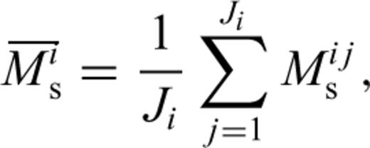
where J_i is the total number of stations at which event i is observed. We assume that there is a ‘true’ surface-wave magnitude, , which is approximately equal to for large J_i. The scatter of M^ij_s about is then assumed to be due to: (1) path-dependent variation in the constant γ (i.e. variations in the effect of dispersion and attenuation); (2) variations with period, T; and (3) a station term. So we can write:

10

where δγ_p is the variation in γ associated with path p, S_j is the station term for station j, T′= (T−T₀)/(T_max−T_min), T₀ being a reference period and κ a constant. T_max and T_min are the maximum and minimum values of T permitted (here 22s and 18s respectively). Then, assuming that , the residual, d_ij for each event-station pair is given by

11

We assume that we can express γ_p as an integral through a 2-D model expressed in spherical harmonics, i.e.

12

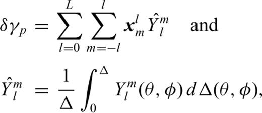
where x is the vector of model coefficients and is the path-average of spherical harmonics along path p. We then have a set of equations of the form

13

where now y is a vector of station terms and z is the correction for period. Writing

14

and

15

this is equivalent to

16

for which we find a weighted solution (Jackson 1972) of the form,

17

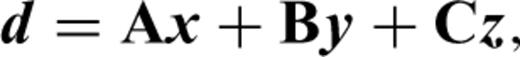
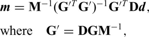
with D a matrix of data weights and M a matrix of model weights. In practice we seek a damped solution of eq. (17) by replacing (G′^TG′)⁻¹ by where and Λ are the set of eigenvectors and eigenvalues of (G′^TG′)⁻¹ respectively, and λ_n is the nth eigenvalue in order of size where n is chosen as a compromise between model size and variance reduction achieved.

3.3 Data weighting

We introduce an a priori data weighting scheme based on an analysis of similar paths. The surface of the Earth is divided into 5°× 5° cells, with the number of paths sharing common starting and finishing squares being N_s. The data weight for path p, D_p is then given by

18

The intention is to give greater weight to the contribution of unusual paths. This is helpful because of the large variability in geographic data coverage, which can be seen from the large variation in arrivals at each station (Fig. 3). The REB includes a time residual relative to model arrival time for Rayleigh wave observations. We investigated the use of this time residual as an a priori measure of data quality but found no correlation.

3.4 Model weighting

Model weighting is an important issue in this type of study. First, we impose the condition that each of the three parts of the model [δγ(θ, φ) distribution, period dependence and set of station corrections] is weighted equally. Second, we apply a smoothness constraint to the spherical harmonic expansion of δγ(θ, φ) where each degree, l, of the expansion is weighted by 1/[l(l+ 1)]² (Trampert & Woodhouse 1995). This weighting reduces the contribution of the shorter-wavelength model components, resulting in a smoother model. However, there is the danger that in areas of poor data-coverage and resolution the amplitude of long-wavelength structure may be exaggerated.

A final point is that we add into the inversion the constraint

19

i.e. the sum of the station terms, weighted by the number of observations at each station, is equal to zero. This prevents the mean of the set of station terms trading-off with the degree zero of the spherical harmonic expansion.

3.5 Modelling procedure

1. An initial inversion is carried out to degree 10 spherical harmonic expansion of δγ(θ, φ) together with a set of station terms and a term for period-dependence. We then calculate the misfit between observation and model prediction for each path. Paths whose absolute misfit is greater than 2.5σ are excluded at this point.

2. 20
   A second inversion is carried out to degree 20. We then calculate the model prediction for each path (station term, period term and path term) and correct each observation. This allows us to produce a recalculated mean for each event, , where:

   

   20

   This step allows for any bias in the original mean due to the path and station corrections, i.e. we assume that is closer to than .
3. 21
   We then recalculate residuals relative to the new mean:

   

   21

   and use these values in a second iteration for a degree 20 inversion.

3.6 Results

The resulting δγ(θ, φ) model is shown in Fig. 6(a). Paths through blue areas give an increased value for M_s whereas paths through orange areas give decreased M_s. There is a clear correlation with tectonic patterns, with continents and ocean basins generally enhancing Rayleigh amplitudes and regions near plate boundaries decreasing amplitudes. The regions of strongest negative δγ(θ, φ) occur in the Mediterranean, Indonesia and the northern Atlantic/Arctic Ocean, and regions of strong positive δγ(θ, φ) are found in continental regions and the central Pacific. However, resolution in the southern hemisphere (particularly in the southern Atlantic and Indian Ocean) and much of the Pacific is poor due to the scarcity of stations, the requirement of at least ten observations of each event, and the limit of 100° on path length.

Figure 6

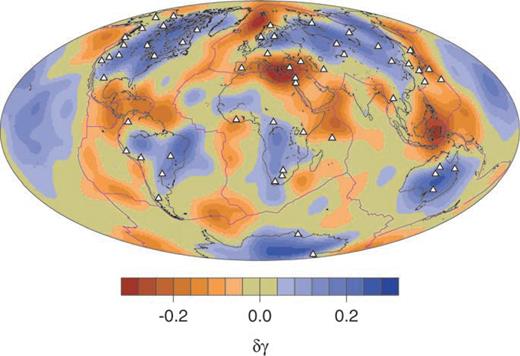
Distribution of δγ(θ, φ). Stations used are shown as white triangles and plate boundaries as purple lines.

Open in new tabDownload slide

The set of station terms range from about −0.1 to 0.15 m.u. (Fig. 7). Stations with relatively few observations are likely to have large residuals (cf. Fig. 3) so these should be treated with caution. However, BOSA, BJT and DBIC each show large positive station terms and NOA and ILAR show significant negative values. Stations CMAR, KSAR and ESDC each have multiple station terms (see Section 2) which can vary greatly (note in particular CMAR and CMAR2). This suggests that changes in instrumentation (or perhaps changes to the total network over time) can lead to large changes in station term, which may mean that relating station terms to local Earth structure is difficult.

Figure 7

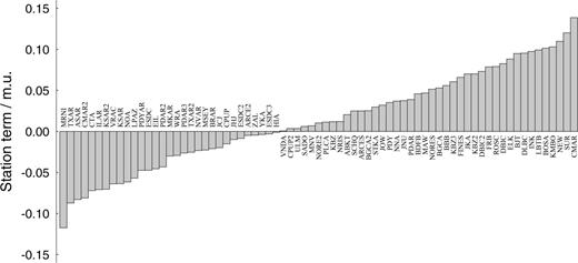
Station corrections in magnitude units (m.u.).

Open in new tabDownload slide

Finally, we find κ=−0.05, which indicates that there is a systematic trend of measured M_s with T, with measurements made at 22s being on average 0.05 m.u. lower than those made at 18s. However, we also find that measurements made on continental paths are likely to be at shorter periods than those made elsewhere, so this value may not be independent of the δγ(θ, φ) distribution.

Table 2 lists the variance reductions achieved for each stage of the modelling process and the variance reduction due to each part of the model. Note that since the model parameters are not orthogonal, there is no requirement that V_total=V_path+V_station+V_period. In Table 3 we list the equivalent variance reductions for an alternate set of models where we included no data weighting. The variance reductions achieved are similar.

2

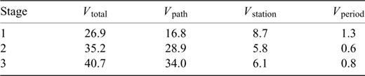
Variance reductions achieved for the M_s correction model. V_total is the variance reduction achieved for the total model, and V_path, V_station and V_period the variance reduction achieved by the δγ(θ, φ) distribution, station corrections, and period correction respectively.

Open in new tabDownload slide

3

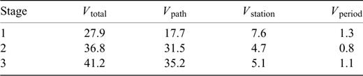
Variance reductions achieved for an alternate model in which data weights were not included, see text for details. Column headings as for Table 2.

Open in new tabDownload slide

4 Discussion

Currently the IMS network is probably insufficient to recover a fully accurate model for M_s corrections. The sparse station network in the southern hemisphere and Pacific region together with the restriction of path length Δ≤ 100° and the requirement for at least 10 stations to record each event mean that data coverage is poor in many areas of the globe, both in absolute and azimuthal terms, which are equally important in this kind of study.

The uneven data coverage means that the model space is not evenly sampled, which will lead to a posteriori correlations between the spherical harmonic parameters. This means that ‘underdamping’ of the inversion could lead to spurious perturbations in the retrieved model. Although we have attempted to minimize the effect of this problem, a more spatially complete data set is required to completely eliminate it. In addition, it is inevitable that some of the station terms will be correlated with each other and with the spherical harmonic coefficients. This again increases the sensitivity of the model to correlated errors in the data.

However, in regions where coverage and resolution is good (North America, the north Atlantic and Arctic and much of Eurasia) the models retrieved appear to be robust and revealing. If variations in M_s are due to the effects of dispersion and attenuation, then we would expect to see amplitudes reduced in areas of thick sediment or tectonic complexity. Rayleigh amplitudes should be enhanced in stable areas such as old continents and oceans. It is important to remember at this point that M_s is effectively a measurement of the envelope of a seismogram convolved with a particular instrument response or filter. M_s is therefore sensitive to a range of periods around the measurement period determined by the dispersion (group speed curve), amplitude spectrum and filter or instrument response. We should not necessarily expect the resulting model to correlate with existing studies of phase-speed or attenuation.

4.1 Regional biases in M_s

Using our model of path, station and period corrections it is now possible to investigate whether there are systematic regional biases in the estimation of M_s. To test this we use the set of events reported during 1999 which are given an M_s value in the REB, subject to the same data-editing as described above. The model described was constructed using only events for which J_i≥ 10 where J_i is the number of stations observing event i. However, this is only a small sub-set of the events with surface wave magnitude given in the REB. Fig. 8 shows the distribution of J_i for 1999. More than 25 per cent of the events with an M_s have that magnitude calculated from only one observation.

Figure 8

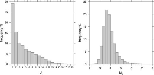
Left: Histogram showing the number of observations used to calculate M_s for events in the REB. For example, around 25 per cent of the events in the REB given an M_s, have that M_s calculated from one observation. Right: Histogram showing the distribution of mean M_s for events used in this study. Note that the majority of the events have mean M_s below 4.0.

Open in new tabDownload slide

We calculate the M_s correction for each observation in the REB and then recalculate for all i. Fig. 9 shows the difference between the original and updated mean M_s (negative values indicate that the original is an underestimate). Most of these differences are between ±0.2.

Figure 9

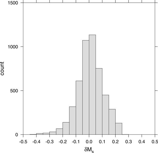
Histogram showing the effect of the model on mean M_s for all events given an M_s during 1999.

Open in new tabDownload slide

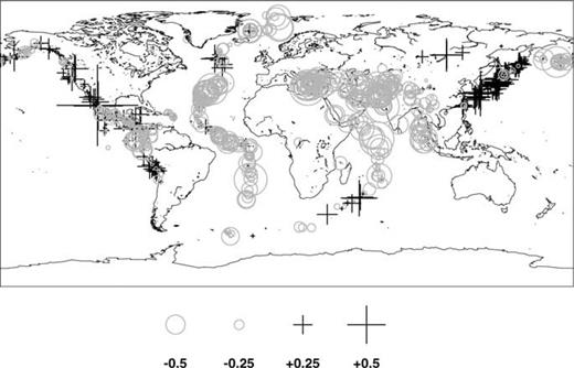
We then investigate the geographic distribution of M_s bias. In Fig. 10 we show the distribution of events for which the . Black crosses indicate events for which the revised magnitude is smaller than the original. We see that the original M_s was overestimated in regions such as central Asia, the western margin of North and South America, Japan and the Tonga-Kermadec trench region. The grey circles show that events in the eastern Mediterranean and Middle East as well as those in Indonesia are underestimated if the corrections are not used.

10

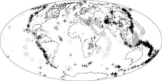
The change in for events during 1999. Black crosses indicate events for which the model decreases , i.e. the raw data overestimates . Grey circles indicate events for which the modelling process increases .

Open in new tabDownload slide

4.2 Possible effect of data censoring

Surface wave observations are required to pass a dispersion test before M_s can be reported in the REB (Stevens & McLaughlin 2001). This means that any surface waves which deviate greatly from the model group speed predictions will not be included. If, as we assume, M_s residuals are at least partly related to the shape of the group-speed curve for a path, then the observations of amplitude are not independent of the group-speed model, i.e. amplitudes will not be measured for paths which do not fit the group-speed model, producing a data-censoring effect. However, we feel that this is a weak effect since the time window used in association with the group-speed curves is wide enough to allow any genuine surface wave to be detected. The censoring effect is certainly not comparable to that in any study which utilizes a waveform-fitting technique of surface-wave measurement.

4.3 Remaining residuals

The modelling process above accounts for around 40 per cent of the variance of the observations, and so a large part of the observations are not explained by the model. In Fig. 11 we show the effect of the modelling on the observed station residuals. The top panel shows the observed residuals for station NOA in southern Norway, plotted in the same way as Fig. 5. In the middle panel are the model predictions. Although the general pattern of the predictions matches the observations, the size of the residuals is generally smaller. This is presumably because of the trade-off with observations at other stations. The bottom panel shows what remains of the observations after modelling. there are still distinct patterns of residuals, particularly in the western Pacific and Atlantic regions. These residuals are not explainable within the framework outlined above. We surmise that these residuals are due either to path effects which cannot be predicted by our model—for instance, there may be systematic effects on amplitude dependent on the angle of intersection between the path and an ocean/continent boundary—or to the effects of source radiation pattern. However, preliminary attempts to match radiation patterns from earthquakes with known mechanisms to either the initial observations or the residuals after modelling have proved inconclusive, so this question remains to be resolved.

11

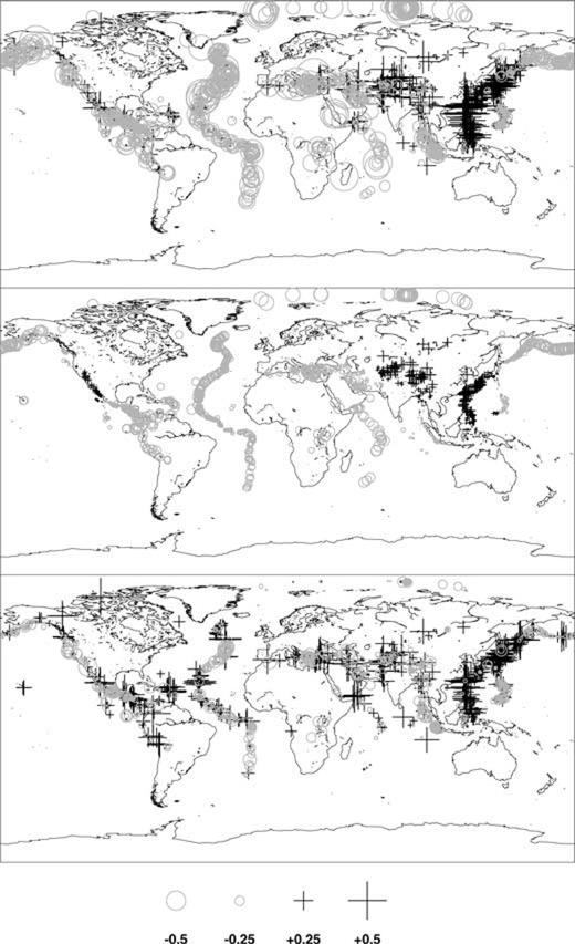
The effect of the modelling process on M_s residuals observed at station NOA, Norway. Top: Observed M_s residuals. Middle: Model predicted residuals. Bottom: Difference between observed and predicted residuals. Distinct clusters of positive and negative residuals are still visible.

Open in new tabDownload slide

5 Conclusions

M_s residuals show systematic patterns which can, at least in part, be attributed to lateral variations in Earth structure. Determining reliable M_s path corrections is potentially vital since event screening and discrimination can depend critically on the use of the m_b: M_s criterion. If the number of M_s observations is very low, which is likely to be so for small explosions, then path and station dependent effects can potentially bias the observed M_s of a seismic disturbance. However, it is critical that any postulated M_s corrections are not contaminated by earthquake radiation pattern effects since these would not be applicable to explosions. Hence, using the raw data, ‘source-station specific’ type corrections will probably be contaminated more by radiation pattern effects than this type of model. Also, station corrections for M_s need to be de-sensitized to the effects of path-dependent variations in M_s, so that they can be applied with equal validity to events happening in any region of the Earth. A joint inversion such as is described here can go some way to achieving this.

The type of results presented here are potentially beneficial in studies of Earth structure, and complementary to group-speed studies using Rayleigh waves of similar periods (see, for example Ritzwoller & Levshin 1998; Vdovin 1999). As the IMS network grows, and if, as has been suggested, greater efforts are made to retrieve long-period data from IMS auxiliary stations, our understanding of M_s residual distribution across the Earth can only improve.

This paper does not discuss the relationship between M_s and M₀, which has been discussed elsewhere (e.g. Ekström & Dziewonski 1988; Herak 2001). We also do not discuss the relationship between M_s and the yield of explosions (e.g. Marshall 1971; Stevens & Murphy 2001). However, the results presented here suggest further work which may improve our understanding of these relationships.

A final word of caution is that the results in this study can only be guaranteed to apply to M_s measurements made using the methodology of Stevens & McLaughlin (2001) described above. Surface waves generated from small, shallow explosions have a different character to earthquake data (having a much higher frequency content) and so may require a more appropriate method of M_s measurement (such as that described by Marshall & Basham 1972) which would require frequency-dependent path and station corrections.

Acknowledgments

The figures in this paper were produced using GMT (Wessel & Smith 1998). The authors would like to thank the staff of the pIDC, IDC and IMS responsible for producing the data utilized here.

References

Footnotes