


Summary
In most marine sedimentary records, the Matuyama-Brunhes boundary (MBB) has been found in interglacial oxygen isotope stage 19. In the magnetostratigraphic records of most Chinese loess/palaeosol profiles the MBB is located in loess layer L8, which was deposited during a glacial period. The MBB at Lingtai (central Chinese Loess Plateau) also occurs in L8 and is characterized by multiple polarity flips. The natural remanent magnetization is mainly carried by two coexisting components. The higher coercivity (harder) component dominates in loess layers and is thought to be of detrital origin. The lower coercivity (softer) component prevails in palaeosols and was most probably formed in situ by (bio-)chemical processes. A lock-in model for the Lingtai MBB record has been developed by extending the lithologically controlled PDRM model of Bleil & von Dobeneck (1999). It assumes two lock-in zones. The NRM of the magnetically harder component is physically locked by consolidation shortly after loess deposition, whereas the softer component is formed at greater depth by pedogenesis and acquires a chemical remanent magnetization of younger age. At polarity boundaries, grains carrying reversed and normal directions may therefore occur together within a single horizon. The model uses ARM coercivity spectra to estimate the relative contributions of the two components. It is able to explain the observed rapid multiple polarity flips and low magnetization intensities as well as the stratigraphic shift of the Lingtai MBB with respect to the marine records.
1 Introduction
The Matuyama-Brunhes boundary (MBB) has been observed in many sediment cores from different oceans. Tauxe (1996) compiled 19 such records with sedimentation rates of up to 8 cm kyr−1 and confirmed that the MBB occurs in most cores in sedimentary layers representing the interglacial oxygen isotope stage 19. Astronomical calibration of the marine oxygen isotope record places the MBB at 778.8 ± 2.5 ka (Tauxe 1996). This date agrees well with radiometric ages derived from volcanic sequences, which give 778.2 ± 3.5 ka (Tauxe 1996) or 780 ± 10 ka (Spell & McDougall 1992) as the best estimate. Tauxe (1996) also reported that the natural remanent magnetization (NRM) in marine sediments is fixed within a few centimetres of the water-sediment interface. Among others, deMenocal (1990) and Bleil & von Dobeneck (1999), report downward shifts of magnetic polarity boundaries in marine sediments, with values ranging of 7 to 17 cm.
Surface layers of marine sediments are commonly unconsolidated due to high porosity and frequent bioturbation in the upper 5–15 cm. An acquired depositional remanent magnetization (DRM) cannot persist under these conditions (Guinasso & Schink 1975). According to the widely accepted concept of a post-depositional remanent magnetization (PDRM), the magnetization is gradually locked below this unstable layer after a certain amount of overburden has accumulated on the palaeosurface (Irving & Major 1964; Kent 1973; Otofuji & Sasajima 1981). Because the post-depositional fate of each magnetic particle is of a statistical nature, any magnetic assemblage will exhibit a distribution of different individual lock-in depths – even under the most idealistic assumption of uniform magnetic and non-magnetic matrix particle sizes. The macroscopic process is therefore appropriately described by a ‘lock-in zone’ (Løvlie 1976; Niitsuma 1977) rather than by a sharp ‘lock-in front’. Consequently, lock-in not only delays remanence acquisition with regard to sediment age, but it also acts as a smoothing filter in the depth and time domains. Effects of delayed and gradual recording upon the palaeomagnetic fidelity of homogeneous sediments have been mathematically investigated by Denham & Chave (1982) and Hyodo (1984).
Bleil & von Dobeneck (1999) defined the initial lock-in depthd0 as the depth above which no lasting magnetization is acquired. Under simple assumptions, a magnetic polarity boundary appears in the record where 50 per cent of the magnetic moments have been blocked parallel to the old polarity, and 50 per cent of the moments are blocked parallel to the new field polarity. The corresponding depth is called the median lock-in depth . The depth where all available magnetic particles have been fixed is the total or terminal lock-in depthd1.
If lock-in is regarded as a steady-state process, brief polarity intervals will be recorded only if they last longer than the median lock-in depth divided by the sedimentation rate. Therefore, short-lived geomagnetic events may not impart a clear polarity imprint on a PDRM record.
Terrestrial loess sediments also record geomagnetic field behaviour. Loess sequences consist of loess/palaeosol alternations where loess layers are relatively fresh aeolian deposits formed during colder climate periods, whereas palaeosols develop on a loess layer by pedogenic processes during warmer and wetter conditions. Heller & Liu (1982, 1984) observed the MBB at Luochuan (central Chinese Loess Plateau, CLP) in the 8th palaeosol (palaeosol S8) from the top of the sequence. Many other authors observed this boundary in the more recently deposited loess layer above S8 (called L8 according to the nomenclature of Liu & Chang 1964). Sometimes the MBB was not noticed at all in this entire stratigraphic interval (Hus & Han 1992). Hus & Han (1992) pointed out that different PDRM lock-in depths could explain the different stratigraphic positions of the MBB. There is now overwhelming evidence that the MBB on the Chinese Loess Plateau is recorded mostly in loess layer L8 (Liu 1988; Cao 1988; Rolph 1989; Rutter 1990; Zheng 1992; Li 1997; Ding 1998; Zhu 1998; Spassov 2001).
Variability of lock-in depths may be due to different post-depositional processes. The fixing of magnetic grains in loess depends on the stabilization of the sediment microstructure. After the settling of the dust particles, ‘loessification’ (transformation of dust into loess coupled with secondary calcification) establishes this microstructure. This structural change takes place in a depth zone between ∼0.4 and <1 m under specific loading and wetting conditions (Assallay 1998). In addition, the presence of oxidized titanomagnetites (Heller & Liu 1984), the alteration of unstable minerals (biotite, augite) in strongly weathered loesses (Liu 1985) and the reductive dissolution of iron which can be reprecipitated in oxidizing or carbonate-rich environments (Perel’man 1977) would also argue for the formation of a chemical or crystallization remanent magnetization (CRM).
Based on a detailed stratigraphic comparison between neighbouring loess/palaeosol sections of the central CLP, Heller (1987) suggested local relative remanence lock-in delays of about 20 kyr for the MBB and proposed a correlation of palaeosol S7 with marine oxygen isotope stage 19. Zhou & Shackleton (1999) compared the MBB records of deep-sea cores and other (lacustrine) continental sediments and concluded that the MBB should be observed within oxygen isotope stage 19. They considered the MBB position in the marine sediments as a reliable time marker and argued that the MBB in the loess sediments at Luochuan, the classical section on the CLP, was displaced downward by 1.7 to 2.5 m and that oxygen isotope stage 19 should be correlated with palaeosol S7. They used the 700–800 ka old Australasian micro tektite layer, which was observed in deep-sea cores about 12 kyr before the MBB (Schneider 1992; Kent & Schneider 1995), to fix their correlation in an absolute time frame. Some microtektites have also been identified in the upper part of L8, but above the recorded MBB (Li 1993).
The Chinese loess/palaeosol timescale developed by Heslop (2000) is based on the correlation of astronomically tuned monsoon records with the oxygen isotope record of ODP site 677 (Shackleton 1990). Heslop (2000) concluded that the polarity boundaries are displaced and shifted downward in the loess stratigraphy. They arrived at shift estimates of 1.90 m at Baoji (central CLP) and 1.59 m at Luochuan, which would correspond to time delays of 26 and 23 kyr, respectively, and they also suggested a correlation of palaeosol S7 with marine oxygen isotope stage 19 (see also Evans & Heller 2001).
The present study is intended to shed some light on the processes, which cause the apparent time lag of the MBB in the Chinese loess sediments with respect to the marine record. The loess section at Lingtai (central CLP) has been selected for detailed rock- and palaeomagnetic measurements. Post-depositional and chemical processes of remanent magnetization acquisition will be considered in the development of a lock-in model, which extends the PDRM model proposed by Bleil & von Dobeneck (1999).
2 Magnetic Polarity Boundaries and Rock Magnetic Properties of the Lingtai Section
The Lingtai section (107.56°E, 34.98°N) is located in the central part of the CLP. The upper 175 m of the 305-m-thick section consists of alternating loess/palaeosol and the lower part is formed by Mio-/Pliocene red clay with a basal age of about 7.05 Ma (Ding 1998). Some 32 palaeosols have been identified in the Lingtai sequence. They can be correlated with other sections, for instance with Baoji (Rutter 1991), and provide a complete stratigraphic sequence. The Lingtai section was sampled continuously from 0 to 268.12 m, resulting in about 13, 400 oriented cubic samples with an edge of 2 cm.
Here we discuss results from samples spanning the MBB. A first sample set (set A) was collected to provide continuous data for a 3 m stratigraphic interval from S8 through the slightly weathered L8 up to S7. All samples from set A were stepwise thermally demagnetized. Another independent sample set (set Y, collected about 1 m away from set A) was treated using alternating fields (AF) demagnetization. A secondary present-day overprint was removed at temperatures between 250°C and 300°C or at peak fields of 15 mT or 20 mT in both loess and palaeosol samples. After demagnetization treatment the MBB was found between 61.4 and 62.0 m in L8 (Fig. 1), implying an average sedimentation rate of 7.9 cm kyr−1 for the Brunhes part of the section.
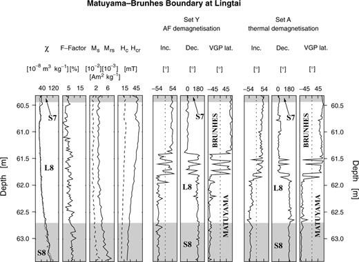
Continuous magnetic records across the MBB boundary at Lingtai (central CLP). The directional behaviour of the MBB transitional polarity interval (given by ChRM declination, inclination (local geocentric axial dipole inclination = 54°) and VGP latitudes, respectively) is characterized by seven full polarity changes in both data sets. Two intermediate VGP positions are located at depths 61.94 m and 62.20 m in set Y. A slight stratigraphic shift of the transitional directions is seen between thermally and AF demagnetized data. Low field susceptibility (χ), frequency dependence of susceptibility (F-factor resulting from measurements at two frequencies, 0.47 kHz and 4.7 kHz), coercivity Hc (dotted line), coercivity of remanence Hcr (solid line), saturation magnetization Ms (maximum field of 300 mT; dotted line) and saturation remanence Mrs (solid line). All rock magnetic data are from set Y, except the dotted susceptibility curve, which is from set A. Since both susceptibility curves coincide, stratigraphic consistency of both sample sets is demonstrated.
The stable, characteristic remanent magnetization (ChRM) records seven full polarity changes at the MBB throughout a transitional zone of about 0.4 m thickness. They occur at slightly different depths in the two data sets (Fig. 1). Two intermediate VGP positions are observed in the Y data (AF) within 0.5 m below the lowermost full reversal. They are not present in set A (thermal). The partly dissimilar ChRM directions seem to reflect different demagnetization response of the coercivity and the blocking temperature distributions of the magnetic mineral fractions present.
In order to assess the reliability of the data, the maximum angular deviation (MAD) of the regression line of the ChRM was calculated, using the same number of demagnetization steps (6) for all samples (Spassov 2001). Both demagnetization methods yield approximately the same precision above and below the transition zone with MADs generally <10° whereas the ChRM directions are less well defined within this zone, with MADs sometimes exceeding 30°. This may be due to increasingly mixed ChRM polarity within these samples. The two intermediate VGPs also have high MAD values (Spassov 2001).
Specific low-field susceptibility χ, coercivity Hc, coercivity of remanence Hcr, saturation magnetization Ms and saturation remanence Mrs vary smoothly across this stratigraphic section and do not show any abrupt changes near, or within, the transition interval (Fig. 1). The coercivity values slightly increase from S8 to L8 and suggest that two coercivity populations, coexist in the loess/palaeosol samples (cf.Evans & Heller 1994). Higher concentrations of a rather fine-grained mineral fraction (magnetite) are indicated in palaeosol S8 by higher frequency dependence of susceptibility (F-factors) and saturation magnetizations together with lower coercivities. We argue that the multiple polarity changes, which do not occur completely simultaneously in both data sets, were caused by lock-in effects rather than by geomagnetic field behaviour (see Spassov 2001). They are not correlated with any distinct changes of the rock magnetic signature or lithology. The syn- or post-sedimentary formation of detrital and pedogenic minerals, respectively, may have had an important influence on the lock-in process of the ChRM.
3 Irm Analysis
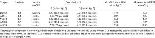
Detailed analysis of acquisition and demagnetization of isothermal remanent magnetization (IRM) data can provide critical information about coercivity distributions and related mineral phases (Robertson & France 1994; Kruiver 2001; Egli 2003). Five samples were selected to investigate the influence of weathering and pedogenesis on the magnetic mineralogy of the loess samples using the technique of Egli (2003). The first sample (BY055) is from the L4 (depth = 69 m) of the high sedimentation rate Baicaoyuan section in the western CLP. It has a low susceptibility of 38 × 10−8 m3 kg−1 and is regarded as being essentially unaltered and unaffected by weathering (see Evans & Heller 1994). The second sample (A1515, depth = 30.3 m) originates from L4 of the Lingtai section. Although this sample is from the central CLP, where sedimentation rates were lower and weathering and pedogenic alteration is generally stronger, it has an even lower susceptibility of only 21 × 10−8 m3 kg−1. The third sample (Y0030) is from the upper part of L8 (depth = 60.9 m) at Lingtai and has a susceptibility of 26 × 10−8 m3 kg−1. The most mature stage of pedogenesis within the interval of interest is expected to be seen at Lingtai in sample A2980 from the weakly developed palaeosol S7 (depth = 59.6 m). Its susceptibility is 77 × 10−8 m3 kg−1. Sample A0494 originates from one of the most strongly developed palaeosols at Lingtai–palaeosol S1 (depth 9.88 m). It has a susceptibility of 215 × 10−8 m3 kg−1.
Preliminary IRM acquisition curves up to 4600 mT saturate at about 3000 mT for loess samples and at 1500 mT for palaeosols. Since the experiments described below involved IRM’s acquired in fields up to 300 mT we will be concerned only with the low coercivity mineral content. This seems to be acceptable as the increase of the IRM acquisition curve above 300 mT is small in both lithologies. In palaeosol and loess samples 93 per cent and 85 per cent of the saturation remanence are reached at 300 mT, respectively.
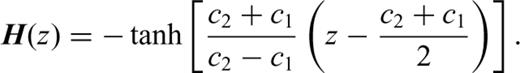
All samples were first demagnetized using an AF of 300 mT along three orthogonal axes. The samples were then magnetized with a DC field of 300 mT along one axis. Tests on samples with different amounts of viscous remanence carriers show that after a waiting time of about 3 min almost no decay of the IRM was observed within the time required for the measurement to be completed. After this delay, stepwise AF demagnetization (logarithmic steps up to 300 mT) of the IRM was performed along the magnetized axis was started and the remaining IRM was measured using a 2G Enterprises cryogenic magnetometer with an in-line AF demagnetization coil. The differential IRM demagnetization curve was calculated using the following steps. First, the original curve was scaled resulting in a linear demagnetization curve. Next, the scaled demagnetization curve was fitted with a hyperbolic tangent function. Then the residuals between the fit and the data were low-pass filtered (using the same Butterworth filter parameters (order 8) for all demagnetization curves) in order to eliminate experimental noise. After backward transformation, a noise-free IRM demagnetization curve was obtained. This curve was then scaled using a logarithmic field scale (base 10), thus the field axis becomes unitless. The resulting derivative, also called the logarithmic coercivity spectrum (LCS), therefore has the same units as the magnetization (for a complete description of the method see Egli 2003).
The initial IRM demagnetization curves show progressively higher intensities with increasing degree of weathering (Figs 2a and b). All IRM gradient curves exhibit a coercivity component that peaks between 40 and 58 mT, which is attributed to minerals of detrital origin (Figs 2c and d). A lower coercivity maximum develops progressively from L4 at Baicaoyuan (BY055) to L8 at Lingtai (Y0030) into the palaeosols S7 and S1. The low coercivity peak is located between 16 and 25 mT. This peak appears to be caused by pedogenic processes as demonstrated by its dominance in the spectra from palaeosols S7 and S1. The higher coercivity component of S7 (dashed line in Fig. 2d) has essentially the same amplitude as that of the parent material in L8.
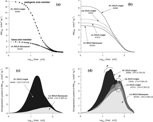
(a/b) AF demagnetization of IRM given at 300 mT for different loess/palaeosol samples. (c/d) Gradients of the demagnetization curves. The higher coercivity component (maximum 40–58 mT) is present in all samples (even in the strongly developed palaeosol S1) and represents the detrital population D, assumed to be uniform across the Chinese Loess Plateau (Evans & Heller 1994). With increasing humidity the loess is affected by weathering and a new low coercivity population P of (bio)chemical grains is formed. The contribution of each component is given in Table 1. The dashed line in (d) represents the continuation of the spectrum of palaeosol S7.
The different magnetization contributions were quantified following the unmixing method proposed by Egli (2003). Magnetizations of mixed components add linearly (Stacey 1963; Kneller & Luborsky 1963; Roberts 1995; Carter-Stiglitz 2001). Therefore the model attributes the coercivity spectra to a number of distinct coercivity populations. Our analysis indicates the presence of one detrital (D) and one pedogenic (P) mineral population. The spectrum for sample BY055 (supposed to represent the pristine loess end-member, see Fig. 2) was subtracted from the spectrum of palaeosol S1 (supposed to represent the pedogenic end-member, see Fig. 2) in order to obtain the pedogenic component P in the sense: P=S1 −n· BY055 (n= 1.5. With this factor, the detrital component disappears completely in the spectrum of S1). After fitting P with a log-normal function, it was subtracted again from BY055 to obtain the pure detrital component: D= BY055 −k·P (k= 0.04. With this factor the pedogenic component disappears in the spectrum of BY055). D was then fitted with log-normal functions. This algorithm was iteratively applied and a stable solution was reached after the second iteration step. Each pilot sample could be modelled using a linear combination of the two components. The area under each gradient curve represents its contribution to the total IRM of the sample. The percentage of the contribution was then obtained by integration of each individual component.
Whereas the detrital component is roughly constant, component P steadily increases from the almost unweathered loess BY055 and peaks in palaeosol S1 where pedogenic minerals show highest concentrations (Table 1). Thus, the contribution of population P varies depending on the stage of pedogenesis. It can also be concluded that the detrital component D is not much influenced by pedogenesis because its contribution in L8 and S7 is nearly equal. As fields up to 300 mT were applied, high coercivity minerals such as hematite or goethite contribute very little to the IRM gradient. The detrital population D (coercivity maximum between 40 and 58 mT) is interpreted as maghemite or titanomagnetite (cf.Eyre 1996), whereas the population P (coercivity between 16 and 25 mT) probably consists of magnetite of chemical or biochemical origin. Referring to magnetite coercivities measured on IRM acquisition curves (Maher 1988), the coercivity values for P are close to the magnetite single-domain/superparamagnetic boundary and single domain state, respectively. These attributes have to be considered with caution since AF demagnetization of IRM and DC acquisition of IRM are physically different processes and hence result in different coercivity values (Cisowski 1981; Fabian & von Dobeneck 1997; Dunlop & Özdemir 1997).
Isolation of magnetic populations for loess/palaeosol samples.
The IRM results confirm our initial assumptions about the degree of weathering of the different samples. The least altered loess sample (BY055) exhibits essentially no low coercivity peak P, but P is evident in loess Y0030 due to weathering, i.e. increasing pedogenesis. The result of our rock magnetic investigation is in agreement with the results of Sartori (2000) concerning general grain size populations, which indicate preferential formation of small grains (clay size) during pedogenesis. Because the pedogenic magnetic component was formed by chemical diagenesis, it is likely to carry a CRM, which may have been acquired under conditions different to those of the detrital component.
4 Lock-In Models
4.1 The linear detrital-pedogenic lock-in model
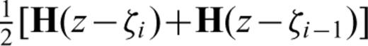
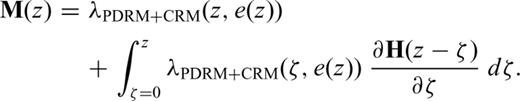
The principles of delayed remanence acquisition have already been discussed, experimentally tested and modelled by Løvlie (1974, 1976), Guinasso & Schink (1975), Denham & Chave (1982), Hyodo (1984), Mazaud (1996) and Meynadier & Valet (1996). Recently, a delayed remanence acquisition model was re-designed and applied to Quarternary deep-sea sediments by Bleil & von Dobeneck (1999). To summarize briefly, a layer, which is now at depth z, was progressively buried under a sediment cover of thickness ζ. During burial the magnetizations of oriented magnetic particles are gradually locked-in. The fraction of the locked magnetic moment can be described by a linear (or, alternatively, curvilinear) lock-in function λ, which depends on burial depth and the lithology.
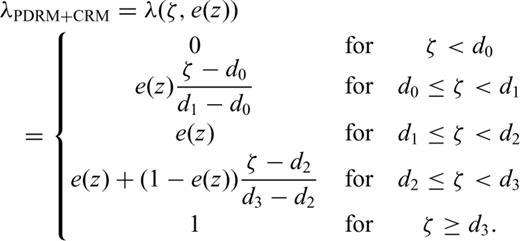

General lock-in function λPDRM+CRM(ζ, e) at a given percentage of the detrital component (e) for the detrital-pedogenic remanence model, which assumes that loess is being deposited and subsequently altered. Until the initial lock-in depth d0 is reached, no magnetization is acquired. The PDRM in the loess is locked completely after d1 has been passed. The loess alteration may have started in the meantime and new magnetic minerals can acquire a CRM at d2. The CRM is totally locked at d3.
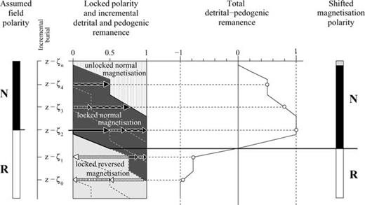
Schematic lock-in process of a two-component (detrital and pedogenic) remanence during a field reversal. The remanence is composed of contributions (arrows) from different discrete lock-in zones separated by the lock-in isochrons (dashed). Equally shaded arrows indicate their affiliation to the respective lock-in zone. A change in magnetic polarity will be observed when more than half of the total magnetic moments are blocked in the new field direction.
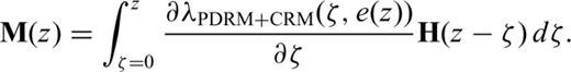
 . The total remanent magnetization M is obtained by multiplying both terms and by summing up the partial remanences (arrows in Fig. 4) of all n steps to ζn=z:
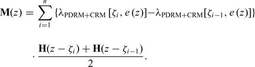
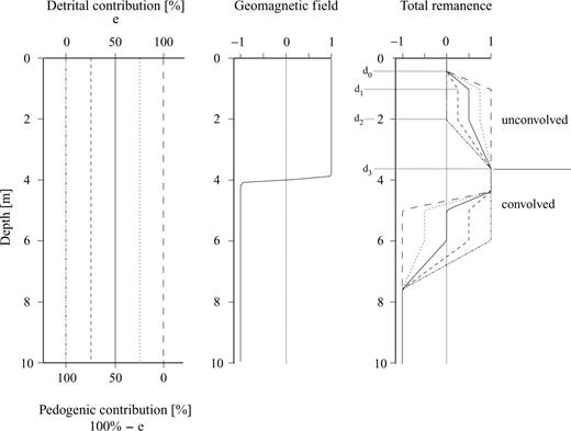
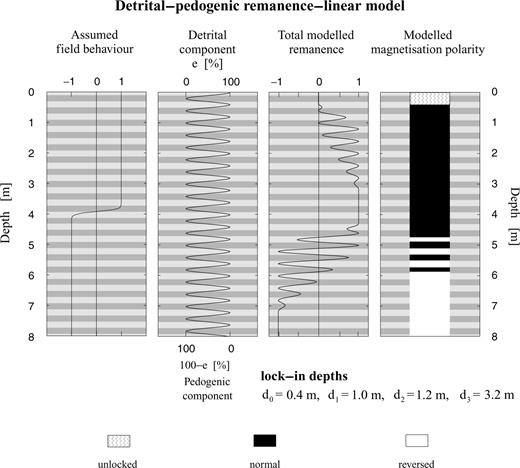
Modelled detrital-pedogenic remanence for different constant detrital contributions. Left: The detrital contribution is constant over the whole model space at five different values (0, 25, 50, 75, 100 per cent). Middle: A geomagnetic field reversal is modelled as a tanh function centred at 4 m depth. Right: The modelled remanence acquisition is divided into two parts. The part from 0 to about 3.5 m describes the lock-in process from the surface. Since the field polarity does not change during this most recent lock-in, the lock-in function is not convolved with the derivative of the geomagnetic field. This part of the remanence simply reflects the lock-in function (first term of eq. 4.6). If the polarity of the field changes during lock-in, the lock-in function is convolved with the derivative of the field. Therefore a distorted image of the lock-in process is obtained (it is convolved). The value of the plateau near 5–6 m depends on the lithogenic ratio e. Small lithogenic variations can easily cause multiple polarity flips of the magnetization, if both mineral components (detrital and chemical) are nearly equally represented.
The model relies on the following assumptions: Each magnetic grain is either locked or free to align its magnetic moment parallel to the external field. The dependence on field strength has not been considered because relevant experimental data are missing. The lock-in function λ depends only on lithology e(z) and burial depth ζ. The lock-in rate for each process is constant (linear model).
4.1.1 Estimation of the model parameters
The model assumes that detrital lock-in starts when a loess layer of thickness d0 has accumulated. This may be due to ‘loessification’ which is known to take place between about 0.4 and 1 m (Assallay 1998); these two values are taken to be appropriate estimates for d0 and d1, respectively. It is assumed that pedogenic remanence carriers may start precipitating already during loess deposition. A pedogenic CRM in those mineral phases may begin blocking shortly after the detrital population has been locked. A small depth difference between d1 and d2 of only 0.20 m was chosen at first, corresponding to a time interval of ∼2500 yr and a value of 1.2 m for d2. A value of 3.2 m was found to be appropriate for d3. This lock-in depth corresponds to half of the MBB shift on the CLP (see Heslop 2000; Zhou & Shackleton 1999).
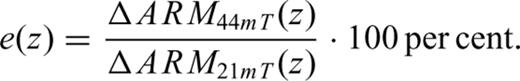
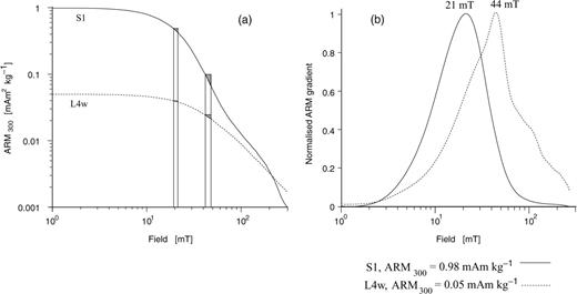
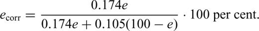
ARM demagnetization curves and ARM coercivity spectra of two samples with different lithogenic properties. Sample S1 is from Lingtai and represents the pedogenic end-member. Sample L4w is from L4 in the Baicaoyuan section (Evans & Heller 1994), western CLP, and is regarded as the unweathered loess end-member. (a) In order to calculate the lithogenic ratio e, the central difference quotients at 21 and 44 mT were chosen to represent the pedogenic and detrital remanences, respectively. (b) The ARM coercivity spectra for the end-members clearly show two separate peaks.
4.1.2 Sensitivity test
Before applying the detrital-pedogenic model to the loess/palaeosol sediments of Lingtai using the measured ARM properties, it was first tested using arbitrary e(z) functions. The lithogenic ratio was assumed to vary sinusoidally between 0 and 100 per cent every 0.2 m over a model space of 8 m. A field change from reversed to normal polarity is supposed to start at 4.15 m and to last for 0.4 m.
First the lock-in function is depicted at a level where sedimentation has stopped at 0 m (Fig. 7). The detrital remanence (peaking in cycles with lighter shading) starts to build-up from zero once d0 has been exceeded. No CRM (peaking in cycles with darker shading) forms at this stage. Below d2 (at 1.20 m), the CRM also starts to lock-in and the PDRM is locked completely with maximum values of 1. The total remanence signal is constant below d3 (3.20 m).
Test of the detrital-pedogenic lock-in model with an artificial lihology. The lithogenic ratio e(z) varies sinusoidally between 0 and 100 per cent every 0.2 m. The modelled detrital-pedogenic remanence changes polarity seven times.
Of course, the lock-in function moves progressively upward with ongoing sedimentation. We start out in the reversed field. Hence, at depth, both components are blocked with reversed polarity. When the field reverses, the lock-in function comes into play and determines the proportion of normally and reversely locked remanence components, respectively. Since the pedogenic component is locked later than the detrital component, it acquires an increasingly normal component that is displaced downward (i.e. it occurs apparently earlier than it should). This holds true also for the detrital component at a later stage or nearer the actual reversal boundary. The convolution of the lock-in function with the field behaviour leads to the recording of seven apparent polarity flips. The normal polarity remanence is completely blocked 0.4 m below the end of the field reversal.
An increase in the period of lithogenic ratio e(z) fluctuations will reduce the number of polarity changes. If the period exceeds 0.86 m (as found by trial and error), only a single polarity change will be recorded. Small changes in the PDRM/CRM ratio occurring near a field polarity change can have a strong effect on the modelled NRM polarity pattern. Model calculations show that a 2 cm thick layer with a detrital contribution of 25 per cent at a critical depth in an entirely pedogenic lithology may create an additional apparent polarity zone.
4.1.3 Model for the Lingtai MBB

Variability of the ChRM intensity indicator (eq. 4.9).
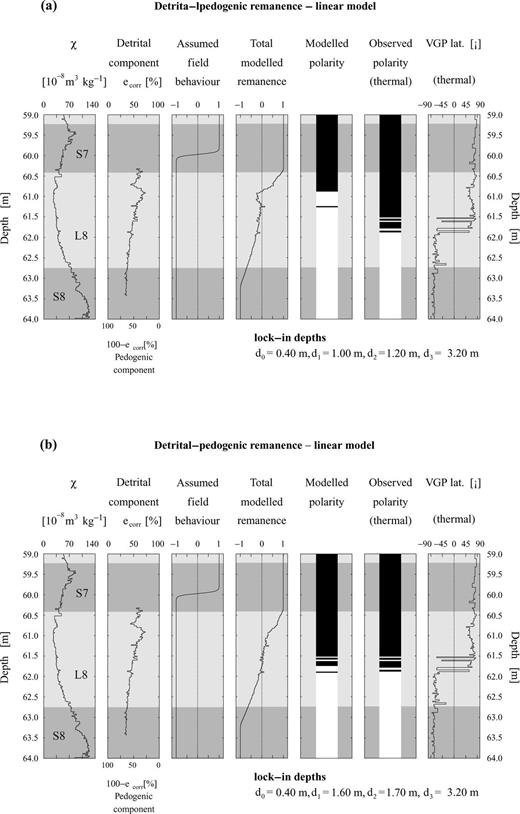
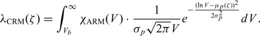
The detrital-pedogenic linear model applied to the loess/palaeosol sediments at Lingtai (central CLP). The changing pedogenic and detrital components cause multiple polarity changes in the modelled remanence. The resolution of the model is 0.02 m. (a) The assumed lock-in depths (see text) do not lead to a good coherence between observed and modelled magnetization polarity flips. (b) Small changes of the lock-in depths lead to an improved agreement with the observed data. The lock-in depths imply nearly equal lock-in rates for the detrital and pedogenic lock-in process. Note that the lithogenic ratio ecorr in loess and palaeosol never accomplishes the values of the ‘pure’ end-members.
The modelled polarity pattern shows some common and some differing features with the observed NRM polarity (Fig. 8a). Three polarity changes occur in L8 between 60.86 and 61.26 m. This is not in agreement with the thermal demagnetization results. Hence, the initially assumed lock-in depths have been slightly modified to improve agreement with the observed data. The best-fitting lock-in depths are d0= 0.4 m, d1= 1.60 m, d2= 1.70 m and d3= 3.2 m (Fig. 8b). After model recalculation, seven polarity changes between 61.48 m and 61.80 m occur. Now, the difference between the midpoints of both multiple magnetization polarity intervals is only 0.03 m.
4.2 The exponential detrital-pedogenic lock-in model
The linear lock-in model is a first-order approximation for remanence acquisition processes on the CLP. Several authors have suggested that exponential lock-in rates may be much closer to reality (Verosub 1977; Hamano 1980; Denham & Chave 1982). In the following, an attempt is made to consider some physical processes for the lock-in process in order to approach a more realistic model.

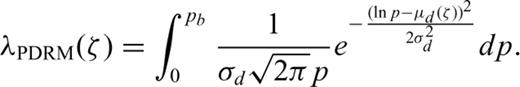
(a) Log-normal distribution of pore sizes. Below a certain pore size, the grains are mechanically fixed and the magnetization is blocked (left, shaded area). (b) Mean of the distribution as a function of burial depth; initial value: pi. Below a certain depth, the terminal pore size pt is reached. (c) The percentage of blocked grains calculated by integration from 0 to the blocking pore size pb. The detrital remanence starts blocking at d0= 0.70 m and is locked at d1= 1.76 m. (The lock-in depths correspond to the best-parameters of the exponential model, see Fig. 11b.)
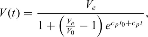
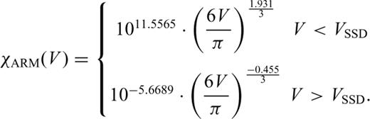
 with Ve denoting the end volume:
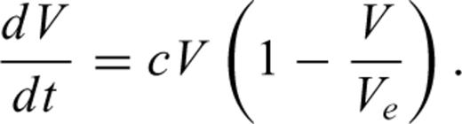
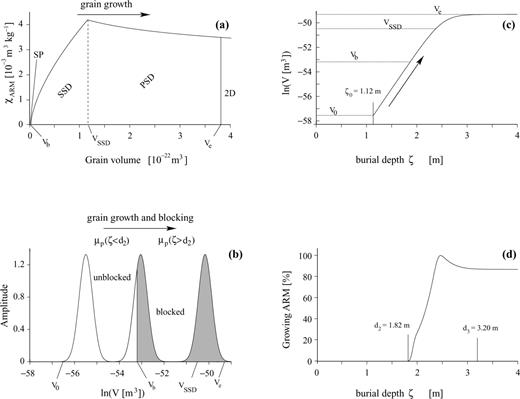
(a) ARM susceptibility (χARM) of magnetite as a function of grain volume. χARM increases within the single domain range. Above 1.13 × 10⁻²² m3 (0.06 μm diameter) the pseudo-single domain stage (PSD) is reached and χARM slowly decreases. (b) Magnetic grains below Vb cannot retain a remanent magnetization (left), and are not blocked. A log-normal distribution of chemically formed grains grows through the blocking volume Vb (arrow). The blocked grains reach the end volume V=Ve. (c) Assumed mean magnetite grain volumes with increasing burial depth. Grain growth stops below a certain depth and the grains reach their final two-domain (2-D) volume of 3.82 × 10⁻²² m3 (diameter = 0.09 μm). (d) The growing ARM is represented by the integral of the distribution multiplied with χARM between Vb and infinity. Because of the decrease of χARM above 1.13 × 10⁻²² m3, the contribution at large ζ is less than at the maximal value VSSD and is taken as the characteristic value for the equivalent CRM. The lock-in depths and ζ0 correspond to the best-fitting parameters of the exponential model (Fig. 11b). In this model, grain growth starts at ζ0= 1.12 m and CRM blocking begins at d2= 1.82 m. The lock-in process is completed at d3= 3.20 m.
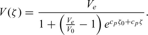
Since sedimentation continues during interglacial stages on the central CLP, burial depth is related to deposition time. Volume growth as a function of increasing burial is shown in Fig. 10(c). The unknown parameters σp, cp, ζ0 were adapted in order to fix the pedogenic lock-in function (Fig. 10d) between the best-fitting lock-in depths d2 and d3 derived from the linear model (cf.Fig. 8b).
Calculating the remanence with this non-linear lock-in function leads to more multiple polarity flips (Fig. 11a) compared to the linear model (Fig. 8b). The non-linear lock-in model, however, does not fit the observed data particularly well and significantly deviates from the best fit of the linear model (Fig. 8b). Changing cd, σd, cp, and ζ0 to 2.55, 0.4, 5.75 m2 and 1.12 m, respectively, yields best-fit lock-in depths of d0= 0.7 m, d1= 1.76 m, d2= 1.82 m and d3= 3.2 m. The results of the exponential lock-in model now become similar to the linear model (Fig. 11b).
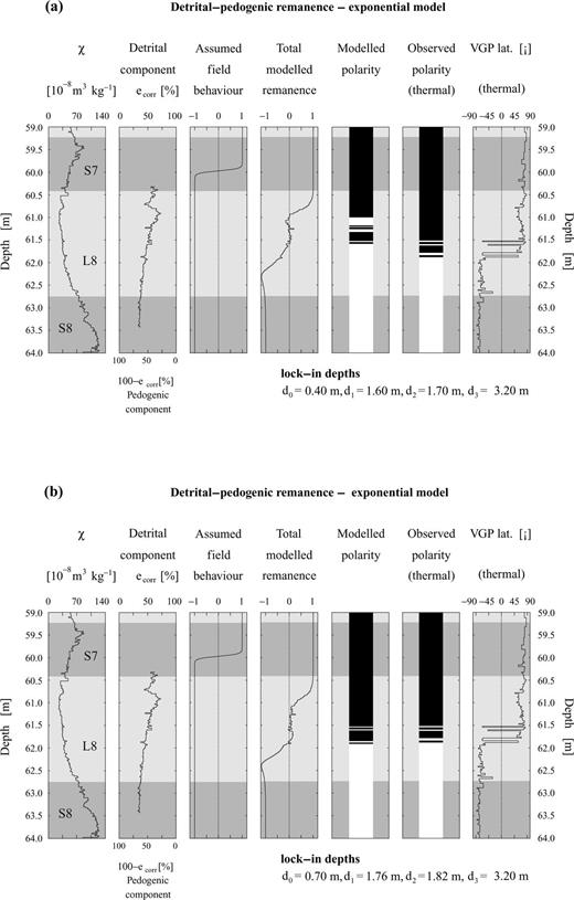
Exponential detrital-pedogenic lock-in model for the loess-palaeosol sediments around the MBB at Lingtai. This model also produces multiple polarity changes. (a) The resulting model zonation differs substantially from the observed polarity pattern and is offset by about 0.5 m when using the optimal lock-in depths of the linear model for the parameter estimation (see text). (b) Optimized parameters lead to different lock-in depths and high similarity between model and observation.
These lock-in depths differ considerably from those initially assumed. In view of their uncertainty, it is not worthwhile discussing their accuracy. The linear and the exponential lock-in models both show that small variations of the lithogenic properties can affect the polarity of the magnetization during a reversal. As pedogenic action on the moist central CLP can start as soon as the loess is deposited, the exponential model may be more realistic.
5 Discussion and Conclusions
Loess is mechanically unstable after deposition. Below a certain depth, it compacts into a more rigid sediment as the transformation of dust into loess, coupled with secondary calcification, builds up a microstructure. This structural change takes place between ∼0.4 and ∼1 m under specific loading and wetting conditions (Assallay 1998), and, among other things, leads to the mechanical fixing of the magnetic grains. Our linear modelling results for the Lingtai section support the idea that the post-depositional remanent magnetization is blocked over approximately this depth zone.
Under sufficiently moist and warm climate conditions, chemical weathering releases iron ions as a basis for the formation of secondary pedogenic iron minerals. Evans & Heller (1994) proposed the coexistence of two magnetic mineral components in loess/palaeosol sediments on the CLP: the primary component is a detrital assemblage of magnetic particles, which appears to be uniform across the entire loess plateau. The second component is an authigenic phase varying between sites and also from layer to layer in a section. The measurements and modelling presented here confirm this suggestion: a low coercivity mineral component (P) is enriched with increasing degree of pedogenesis, whereas the detrital component (D) remains rather constant.
Mineral-magnetic analysis suggests that post-depositional and (bio-) chemical recording processes occur at different stages of burial and therefore at different moments in time and in geomagnetic field history. The relative contribution of the two recording mechanisms has been estimated on the basis of differences in the ARM coercivity spectra. The two lock-in models considered in this paper take both, PDRM and CRM acquisition into account. Piecewise linear lock-in functions lead to a reasonable agreement with the observed data. The exponential model, which seems to be more relevant physically, yields essentially the same results.
Considering that low values and variations of the modelled remanence intensities allow for multiple polarity flips, one could argue that these signal variations are simply random noise. However, the occurrence of a low magnetization intensity zone is an important property of the two component lock-in model if detrital and authigenic carriers contribute at nearly equal proportions (see zero remanence plateau of the 50 per cent PDRM/CRM curve in Fig. 5). Consequently, minor lithogenic variations can easily cause multiple polarity flips, which by no means are caused by rapid geomagnetic field changes. Although the intensity of the magnetic field may also be reduced, the low magnetization zone is mostly due to the lithogenic properties of the sediment and the secondary formation of magnetic minerals. The actual data at Lingtai also exhibit such a zone of low NRM intensity during the MBB transition (Spassov 2001).
A general problem of lock-in processes is the incorporation of depth and time dependent processes. The fixing of magnetic grains in loose sediments depends mainly on the pore size, which decreases with increasing pressure resulting from increasing burial. Therefore the depositional lock-in process depends on burial depth and not on burial time (Bleil & von Dobeneck 1999). The change of the Earth’s magnetic field on the other hand depends on time, not on burial. Thus the calculated magnetization is a function of both time and depth. Several authors simplify the calculations and perform model calculations in only the depth domain (Bleil & von Dobeneck 1999; Hyodo 1984). Calculations in the depth domain are legitimate only for depositional lock-in processes because the transformation from time to depth is linear. This may be not the case for CRM acquisition. The CRM lock-in process depends strongly on the grain volume, which is supposed to increase with time. The burial dependence is indirectly incorporated by assuming ongoing sedimentation of loess during soil development, which is the case in areas of high dust accumulation such as the CLP. Sediment accumulation during soil development and, thus, the indirect burial dependence of CRM acquisition is not well known.
With these precautions in mind, the following conclusions can be drawn from modelling the NRM lock-in process at Lingtai.
The linear detrital-pedogenic remanence model is able to explain the downward shift of the MBB in the loess/palaeosol sequence at Lingtai on the central CLP. A displacement from the stratigraphic expected level of 1.74 m (corresponding to a time delay of about 22 kyr) results from the model considerations. The model further explains the observed occurrence of multiple polarity changes by small variations of closely balanced contributions of the detrital and pedogenic mineral components during the MBB polarity change. The good agreement of the modelled results with the observed data supports the hypothesis of two remanence acquisition processes to be involved in the loess sediments of the central CLP: post-depositional (PDRM) and chemical (CRM) remanent magnetization.
The observed multiple polarity changes of the ChRM component are not features of the geomagnetic field during the MBB. They are caused by variable relative contributions of detrital and pedogenic magnetization components during the reversal, which give rise to irregular polarity lock-in at the MBB. Hence, virtual geomagnetic pole paths during reversals from profiles of the central CLP are not representative of geomagnetic field behaviour.
The actual physical deposition processes are most probably not of a simple linear nature. Therefore an attempt has been made to explain the displaced and complicated MBB by a non-linear lock-in model. This model also explains the downward shift of the MBB and the multiple polarity changes. It is in better agreement with the observations than the linear model. Further fundamental data such as blocking pore size, rate of pedogenic grain growth and lock-in depths are needed to obtain better information about the model parameters. The acquisition process of the NRM also needs to be studied. In addition, the simplistic function of the geomagnetic field during the M/B reversal may be replaced with more realistic data for the Earth’s magnetic field as given for instance by the SINT800 palaeointensity stack (Guyodo & Valet 1999) or by reversal simulations (Coe 2000).
The recognition of a delayed Matuyama-Brunhes boundary in loess/palaeosol sequences on the Chinese Loess Plateau solves their conflict with palaeoclimatic records from the marine realm. Hence the Chinese palaeosol S7 almost certainly corresponds to the marine oxygen isotope stage 19, as postulated by Heller (1987), Zhou & Shackleton (1999) and Heslop (2000).
The linear detrital-pedogenic lock-in model is proposed as a first step in solving delayed remanence acquisition processes in sediments with complex recording histories. It yields promising results in the loess/palaeosol sequences of the central CLP. The model can be tested using other well-defined reversal boundaries and other loess lithologies, for instance, on the western CLP. Further experiments concerning the dynamics of CRM acquisition have to be performed to improve mathematical simulations.
Bleil & von Dobeneck (1999) already demonstrated for marine sediments that pseudo-records of palaeointensities can be obtained just by varying the lithology at low to intermediate sedimentation rates (1–4 cm kyr−1). On the central CLP, two or more magnetic mineral populations with variable relative contributions almost always coexist. Their complex interaction and blocking will hamper or even prohibit useful information on palaeointensity changes, palaeosecular variation and polarity transition features during major reversals and/or excursions.
Acknowledgments
We thank Ramon Egli for his constructive discussions and encouraging comments. Special thanks go to David Heslop and Andrew Roberts for a careful review of the manuscript. This study was financed by Swiss National Science foundation grant No 21-54143.98.
References
The pedogenic component P increases gradually from the relatively unaltered loess BY055 on the western CLP representing cold/arid climate conditions to the altered loess Y0030 on the central CLP where more humid climate conditions prevailed. Maximum pedogenesis within the interval of interest is reached in the palaeosol sample A2980.
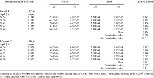
The samples originate from the most pristine loess L4 and well the developed palaeosol S5, both from Lingtai. The magnetic units are given in Am2. The peak AF for the acquired ARM was 150 mT and the bias field 0.05 mT.
