


Summary
A 3-D finite-element simulation of global electromagnetic induction is used to evaluate satellite responses in geomagnetic dipole coordinates for harmonic ring-current excitation of a three-layer mantle overlain by a realistic near-surface conductance distribution. Induced currents are modelled for lithospheric and asthenospheric upper-mantle conductivities in the range σ= 10−4–0.1 S m−1. The magnetic scalar intensity B is calculated at a typical satellite altitude of 300 km. At short periods, T= 2 and 12 h, the induction signal owing to the near-surface conductance is large when a resistive upper mantle is present, but drops off with increasing mantle conductivity. At longer periods, T= 2 d, the near-surface induction signal is generally much smaller and nearly independent of upper-mantle conductivity. The near-surface induction signal is very sensitive to the electrical conductivity of the lithospheric mantle, but only moderately sensitive to that of the asthenospheric mantle. Induced currents are confined to the heterogeneous surface shell at periods of less than 2 h, and flow predominantly in the mantle at periods of longer than 2 d. In the intervening period range, induced currents are partitioned between the near-surface and the upper mantle. These results indicate the importance of carrying out a full 3-D analysis in the interpretation of satellite induction observations in the period range from hours to days.
Introduction
The determination of upper-mantle electrical conductivity from geomagnetic time variations of external origin is a classic problem in solid Earth geophysics (e.g. Chapman & Price 1930). Traditionally, land-based data have been used (e.g. Banks 1969; Schultz & Larsen 1987), but the task is a difficult one since observatories are sparsely and irregularly distributed over the globe and data quality is variable.
Satellite-borne magnetometers provide an intriguing source of information owing to the good spatio-temporal coverage of a long-term orbit. The POGO and MAGSAT data sets from the 1970s and 1980s are now being augmented by scalar B and vector B data from the Øersted and CHAMP satellites. These data sets may prove particularly useful at periods ranging from a few hours to a few days, where good global coverage from observatory data is lacking. Much progress has already been made in extracting induction signals from satellite data (Didwall 1984; Oraevsky et al. 1993; Olsen 1999; Constable & Constable 2000; Tarits 2000; Tarits & Grammatica 2000).
This paper demonstrates that the common assumption of a radially symmetric Earth is a poor one and leads to erroneous determinations of mantle electrical conductivity. 3-D induction is important, especially at periods of less than T∼ 2 d where it is likely to manifest as vertical ‘leakage currents’ into the mantle from the outermost heterogeneous shell of oceans and continents. At longer periods, perhaps beyond the scope of satellite data, strong lateral variations in upper-mantle electrical conductivity will also generate large 3-D induction effects (Weiss & Everett 1998), but this is not of primary concern here. The effects of near-surface conductance on ground-based geomagnetic observations have been studied recently in a global context by Takeda (1991, 1993), Tarits (1994) and Kuvshinov et al. (1999, 2002).
Geomagnetic Induction
There are many lines of evidence to suggest that to first order the near-Earth magnetospheric field, except during some phases of geomagnetic storms and at auroral latitudes, is that of a symmetric ring current aligned with the geomagnetic dipole equator at roughly 3–4 Earth radii (Daglis et al. 1999). The instantaneous strength of the ring current is conventionally monitored by the Dst index, an average of the horizontal magnetic field at a collection of geomagnetic observatories located at equatorial latitudes. The satellite magnetospheric signal, defined herein as the residual scalar intensity B that remains after core, lithospheric and ionospheric contributions are removed, comprises some 20–100 nT (Langel et al. 1996).
The total magnetospheric signal consists of a primary term owing to the ring current itself, plus an induced term from eddy currents inside the Earth responding to fluctuations in ring current intensity. In geomagnetic dipole coordinates, the magnetic-field signal induced by a zonal external current source in a radially symmetric Earth follows a zonal distribution, adding roughly 20–30 per cent to the primary signal at the dipole equator, cancelling up to 80 per cent of the primary signal near the geomagnetic poles. This is easily demonstrated by an analytic calculation of the response of a conducting sphere in a uniform magnetic field. Similar computations have been made in the mining geophysics literature (e.g. Wait & Spies 1969).
Even when the source has a simple spatial structure, induced currents in reality are more complicated since they are influenced by Earth's heterogeneous conductivity structure. The resulting 3-D induction effects at satellite altitudes caused by the spatially complicated induced current flow can be large and dependent on upper-mantle electrical conductivity, as we demonstrate here, so that a complete 3-D analysis of satellite induction data is required for accurate interpretation.
A primary scientific goal of geomagnetic induction is to identify and interpret large-scale variations in upper-mantle electrical conductivity. This is important because, while seismology can ascertain bulk mechanical properties, electromagnetic induction data reflect the connectivity of minor constituents such as graphite, fluids and partial melt, all of which may have a profound effect on primary geochemical fluxes, rheology, mantle convection and plate tectonic activity.
Finite-Element Analysis
To quantitatively model 3-D induction effects in the geomagnetic field at satellite altitudes, a computer program that simulates 3-D electromagnetic induction in a heterogeneous sphere is needed. Several codes are available to this purpose, each based on a different numerical method: spherical thin-sheet analysis (Fainberg & Singer 1980; Kuvshinov et al. 1999), finite-element analysis (Everett & Schultz 1996; Weiss & Everett 1998), finite-difference analysis (Uyeshima & Schultz 2000) and spectral finite-element analysis (Martinec 1999).


The mesh is a decomposition into tetrahedra of a thick spherical shell (Everett 1997). An inner, conducting shell extends from the core–mantle boundary to Earth's surface while an outer, insulating shell extends from the surface to r0= 3 rE, the approximate location of the ring current, where rE= 6371 km is the modelled radius of the Earth. At Earth's surface, the internal and external potentials are coupled by enforcing continuity of the magnetic field, i.e. B=∇×A=−∇Ψ at r=rE.

The linear system of FEM equations is solved using an incomplete Gaussian elimination procedure, termed the ILU method in Everett & Schultz (1996). The method exploits the sparsity of the FEM matrix by neglecting fill-in. The ILU solver is slow compared with modern Krylov solution methods (Saad & van der Vorst 2000), but it converges in near monotonic fashion for strongly heterogeneous electrical conductivity distributions spanning a wide period range.
The finite-element mesh used in this study has an angular resolution of Δ∼ 5° and contains 41k nodes (corresponding to 109k real degrees of freedom) and 180k tetrahedra. The program requires 430 MB of memory and takes 20 min–2 h of CPU time per period on a dual-processor 750 MHz Pentium III machine. The run time depends on the number of ILU iterations, which in turn depends on the complexity of the conductivity model.

 is simply the vector of the final three coefficients in eq. (6). These coefficients, along with a, are determined by a weighted least-squares (WLSQ) minimization of the functional
The MLSI computation of scalar intensity B is a fully 3-D interpolation; i.e. it is not necessary to distribute finite-element mesh nodes over a surface containing the satellite trajectory. We note that the MLSI algorithm can break down in regions where there are sharp gradients in the interpolant. This is the case, for example, when determining electromagnetic fields inside the Earth in the vicinity of conductivity discontinuities. However, the scalar intensity B outside the Earth is smoothly varying since the scalar potential Ψ(r) satisfies Laplace's equation. Therefore, the MLSI determination of scalar intensity B at satellite altitude is a stable, accurate numerical procedure.
Surface Conductance Map
An important component of the present work is to assess the interaction of Earth's heterogeneous near-surface conductance distribution with the underlying mantle conductivity structure. While this could be done using an idealized geometry, the flexibility of the 3-D forward code suggests a more realistic approach. A global sediment thickness map with a resolution of 1 × 1 deg2 has recently been compiled by Laske & Masters (1997). This map contains seismic parameters discretized in up to three layers: a surface layer up to 2 km thick, an underlying layer up to 5 km thick and, where necessary, a third layer to make up total sediment thickness, which often exceeds 10 km.
The seismic parameters are too poorly constrained to warrant using empirical laws to extract a conductivity function. We chose instead to take the most reliable parameter from the map, sediment thickness, and use heuristic rules for generating conductivity.
The sediment map was augmented by the NOAA ETOPO-5 topographic/bathymetric map smoothed to 1° resolution by Laske and Masters. Earth's surface was divided into three regions based on topography: (1) the ocean basins and continental shelves defined by elevations below sea level, (2) the coastal plains and low-lying continental sedimentary basins defined by elevations above sea level but below 100 m and (3) the continental interiors and highlands above 100 m elevation.
The ocean layer was assigned a conductivity of 3.2 S m−1, the upper two oceanic sediment layers were assigned a conductivity of 0.8 S m−1 and the deepest sediments were assigned a conductivity of 0.02 S m−1. The coastal plain sediments were assigned a conductivity of 0.5 S m−1. The continental sediments were assigned a conductivity of 0.03 S m−1. The balance of the section to a depth of 50 km, representing oceanic and continental igneous rocks, was assigned a conductivity of 0.001 S m−1. Total conductance is easily generated by summing the conductivities and thicknesses of the various sections, the resulting model is shown in Fig. 1.
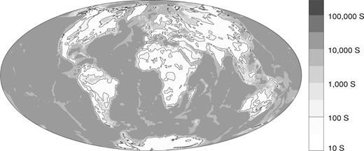
The global surface conductance map derived from smoothed NOAA ETOPO-5 topography and the Laske & Masters (1997)1 × 1 deg2 global sediment thickness map. The conductance is determined by depth-integrating the electrical conductivity in each 1° bin over a 50 km thick spherical shell. Representative conductivity values are chosen for marine, coastal plain and continental sediments, crystalline rock and seawater. The values are given in the text.
Overall, the sedimentary sections defined in this way contribute only 10 per cent to the total near-surface conductance, but in areas such as the Gulf of Mexico, Arctic Ocean and Mediterranean Sea, accumulated sediment has a conductance comparable to the ocean layer. The sedimentary basins cause the large differences between the conductance contours shown in Fig. 1 and the familiar coastlines and shelf contours seen on world maps. A simple averaging scheme was developed to convert the 1°-resolution conductances into 5°-resolution electrical conductivities for the surface layer of finite-element mesh tetrahedra.
Results
The finite-element code was used to simulate global induction by a 1 nT ring-current excitation in geomagnetic dipole coordinates at three periods, T= 2, 12 h and 2 d. A 3-D electrical conductivity model of the Earth was constructed consisting of a three-layer mantle overlain by the global near-surface conductance map. The lower mantle, beneath 670 km depth, is assigned an electrical conductivity of 1.0 S m−1. The upper mantle is divided into ‘lithospheric’ and ‘asthenospheric’ parts, the electrical conductivities of which varied between runs from σ= 10−4 to 0.1 S m−1. The asthenospheric mantle lies between depths of 290 and 670 km. The lithospheric mantle lies beneath the outermost 50 km shell and above the asthenospheric mantle, so it is 240 km thick. It is difficult to model a thin shell using conventional finite-element analysis based on tetrahedral decomposition of a sphere. Thus, the lithospheric mantle and the near-surface conductance are lumped together. Specifically, the lithospheric mantle and near-surface conductances are added together and their sum divided by 290 km to obtain electrical conductivity values for tetrahedra in the mesh layer immediately below the Earth's surface. Finally, the magnetic scalar intensity B at the satellite altitude h= 300 km was calculated using the MLSI post-processing algorithm.
The scalar intensity B at satellite altitude for a resistive upper mantle (lithosphere σ= 10−4 S m−1; asthenosphere σ= 0.001 S m−1) and T= 2 h period is contoured in Fig. 2. The top diagram shows the background, zonal (in geomagnetic dipole coordinates) pattern of induction in the absence of the near-surface conductance map. The induction signal is largest at the dipole equator, adding some 20–30 per cent to the primary ring-current field. Near the dipole poles, the induction signal tends to cancel the primary magnetic field, reducing the total to less than 50 per cent of the primary. The overall pattern is readily understood as arising from a vortex of eddy currents inside Earth that circulates so as to create a secondary field that opposes the inducing field of the ring current, which is uniform and directed roughly southwards along the geomagnetic dipole axis. The outlined contour in the figure is the line B= 1.0, which separates regions of enhanced and reduced scalar intensity caused by induction in the Earth.
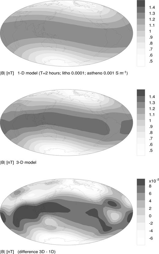
The global scalar intensity B at satellite altitude h= 300 km generated by induction in a model Earth in response to a harmonic ring-current aligned with the geomagnetic dipole equator and fluctuating with a period T= 2 h. The top diagram corresponds to a 1-D Earth model with lithospheric mantle conductivity σ= 10−4 S m−1 and asthenospheric conductivity σ= 0.01 S m−1. In the middle figure, the near-surface conductance map of the previous figure has been added to the Earth model. The anomalous induction response ΔB appears in the lower diagram. It is the difference between the 1-D and the 3-D responses shown above.
The scalar intensity at satellite altitude after adding the near-surface conductance map is shown in the middle diagram of Fig. 2. The pattern suggests a major disruption of induced current in the dipole equatorial region caused by the South American continent, and a smaller disruption caused by the African continent. The induced currents within the continents are reduced in amplitude by the presence of resistive continental rocks. Furthermore, induced currents may preferentially flow in the better-conducting material beneath and/or around these landmasses.
The effect on the global scalar intensity map of adding the heterogeneous near-surface conductance into the model is isolated in the bottom diagram of Fig. 2. The differential intensity map ΔB is obtained by subtracting the intensity shown in the top diagram from the 3-D response shown in the middle diagram. The near-surface conductance effect is certainly large enough (up to 0.1Dst, which is 10 per cent of the primary excitation) to be detected by a satellite magnetometer, and it is strongly correlated with the distribution of oceans and continents. Note that the anomalous currents seem to squeeze between the resistive Southeast Asian and Australian continents, flowing straight through the Indonesian region, which has considerable conductance (see Fig. 1) owing to large sedimentary accumulations and abundant seawater.
The convergence of the ILU solver for the 1- and 3-D models presented in Fig. 2 is indicated in Fig. 3. Note that the convergence is smooth and nearly monotonic with iteration number. The solver appeared to start diverging between iterations 10–50 but soon corrected itself. The cause of this behaviour is being investigated. The 3-D model required approximately twice the number of iterations to converge than did the 1-D model. This is expected since the condition number of the finite-element matrix increases with increasing model complexity, and the rate of convergence scales with the matrix condition number. The ILU solver converged for all the conductivity models considered in this paper.
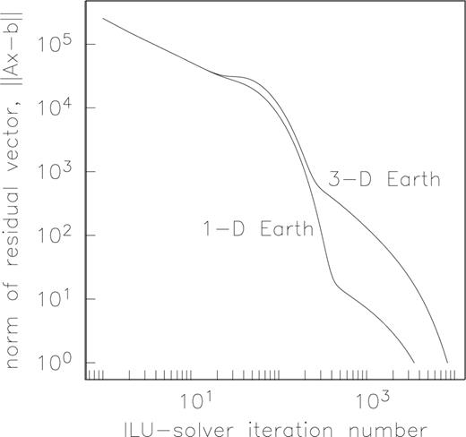
The convergence of the norm of the ILU residual vector as a function of iteration number for the 1- and 3-D Earth models where the responses are shown in the previous figure. Note that the solutions start to diverge but then corrects itself.
The global scalar intensity maps for the same upper-mantle electrical conductivity values are shown in Figs 4 and 5, for periods T= 12 h and 2 d, respectively. The background induction responses (top diagrams of Figs 4 and 5) are similar. The mid-latitude-induced current disruption by continental landmasses is clearly seen in the 3-D response at the 12 h period (middle diagram, Fig. 4). In fact, the disruption is greater at this period than at the shorter 2 d period (cf. middle diagram, Fig. 2). The 3-D induction response for the long-period excitation (middle diagram, Fig. 5) does not exhibit any dipole-equatorial-induced current disruption.
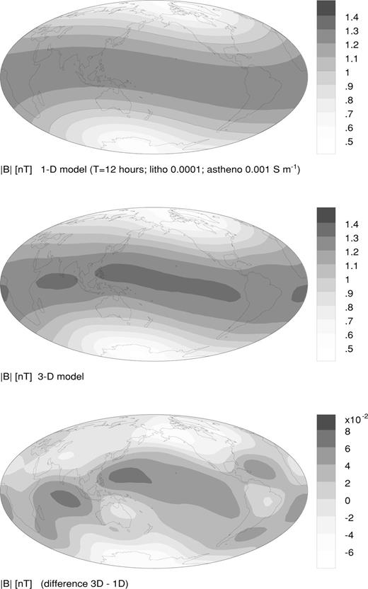
As in Fig. 2, except the period is T= 12 h.
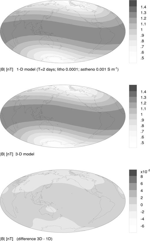
As in Fig. 2, except the period is T= 2 d.
A comparison of the bottom diagrams of Figs 2, 4 and 5 indicates that the size of the anomalous induction signal ΔB decreases with increasing period. This is because the long-period induced current flows beneath the outermost heterogeneous shell. Indeed, the anomalous induction signal at T= 2 d (bottom diagram, Fig. 5) is no longer obviously correlated with the ocean/continent distribution. In the limit as the period T→∞, the ‘dc response’ is attained, which is insensitive to electrical conductivity and depends only on the geometry of the external source.
At long periods (T≥ 2 d), induced currents penetrate deep below the Earth's surface and flow mainly in the good conductor beneath 670 km depth, since the skin depth in the resistive mantle (10−4 S m−1) is some 3 Earth radii. In the case of a conductive upper mantle (0.1 S m−1), the skin depth is approximately 650 km. Ring current fluctuations of the order of 1–3 d, typical timescales for geomagnetic storm recovery, are therefore ideal for probing lateral variations in deep upper mantle and transition zone electrical structure as little distortion from the near-surface conductance is anticipated.
The effect on near-surface induction signals of varying the lithospheric mantle conductivity is shown in Fig. 6. The strength of the anomalous response ΔB decreases as the lithospheric mantle conductivity increases from 10−4 S m−1 (top diagram) to 0.01 S m−1 (middle diagram) to 0.03 S m−1 (bottom diagram). The asthenospheric conductivity is held fixed at 0.01 S m−1. The following explanation is offered. As the upper-mantle electrical conductivity increases, there is less of a contrast in conductivity between the upper mantle and the outer heterogeneous shell. Thus, it is more likely with increasing mantle conductivity that induced currents are not able to discriminate between the outermost shell and the underlying mantle. Consequently, there is less vertical current flow between the mantle and the outermost shell. This vertical current flow may be responsible for much of the anomalous induction signals seen in the models with resistive upper mantles.
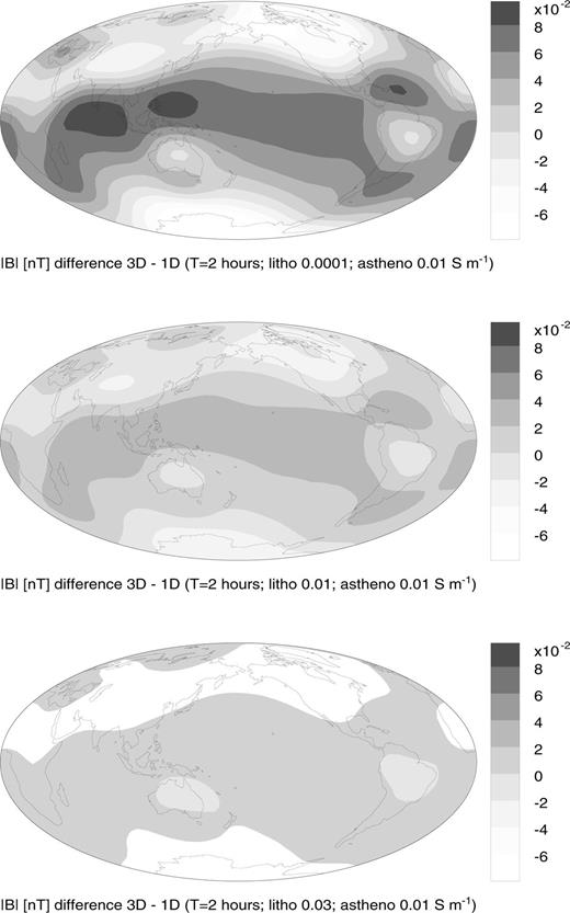
The anomalous induction signal ΔB at satellite altitude h= 300 km above a 3-D model Earth consisting of a three-layer mantle overlain by the near-surface conductance map. A harmonic ring-current excitation of period T= 2 h is applied. The diagrams are shown for various values of lithospheric upper-mantle electrical conductivity.
A more comprehensive analysis of the effect of variable upper-mantle electrical conductivity on near-surface induction signals is shown in Fig. 7. The curves joined by open circles (labelled ‘L’) correspond to models in which the conductivity of the asthenospheric upper mantle is fixed at 0.01 S m−1 and the lithospheric mantle conductivity varies as shown along the plot abscissa. The ‘A’ curves, joined by solid circles, represent models in which lithospheric conductivity is fixed (10−4 S m−1) and asthenospheric conductivity varies. The ordinate ‖Bsec‖ is the ℓ2-norm of the near-surface induction signals. The norm is computed by integrating the anomalous signals ΔB at satellite altitude over the mid-latitudes (±60° latitudes) and all longitudes. Thus, ‖Bsec‖ is a measure of the size of the near-surface induction signal.
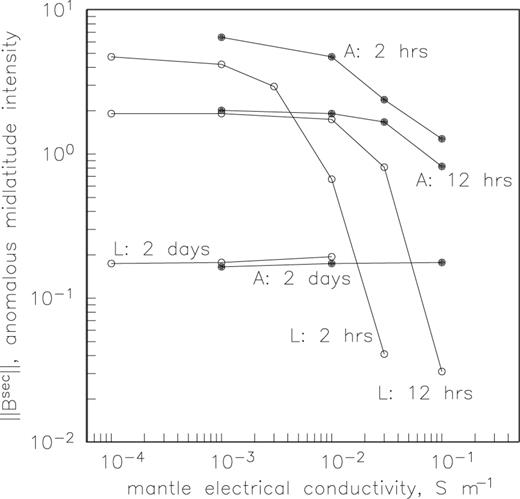
The size of the mid-latitude near-surface induction signal as a function of upper-mantle electrical conductivity, for various periods of ring current excitation. The curves labelled ‘L’ correspond to variable lithospheric mantle conductivity, while the curves labelled ‘A’ correspond to variable asthenospheric conductivity.
Several features of interest emerge from an inspection of the curves shown in Fig. 7. At the longest period, T= 2 d, the size of the near-surface induction signal is small and independent of upper-mantle electrical conductivity. This indicates that the induced currents at this period are flowing in the upper-mantle beneath the outermost heterogeneous shell and also in the lower-mantle conductor.
At the shorter periods, T= 2 and 12 h, a glance at Fig. 7 indicates that the size of the near-surface induction signal is relatively large and independent of mantle conductivity, until the upper mantle becomes rather conductive (σ∼ 0.01 S m−1 and above) in which case the near-surface induction signal diminishes rapidly. This indicates that vertical induced currents flowing between the outer heterogeneous shell and the underlying upper mantle may be important when the latter is resistive. Such vertical currents would be generated where horizontal induced currents are deflected by lateral conductance variations in the near-surface heterogeneous shell. As the underlying medium becomes increasingly conductive, the induced current flow is concentrated mainly in the upper mantle, rather than the outer heterogeneous shell, and there is not as much electromagnetic coupling between them.
Discussion
The utility of this paper for satellite induction studies is predicated on the assumption that the near-surface conductance map shown in Fig. 1 is an adequate representation of Earth's actual conductance distribution. It would therefore be of interest to study the sensitivity of satellite magnetometer responses to perturbations of the near-surface conductance map, especially at short and moderate periods less than T∼ 1 d. This will provide significant information concerning the resolvability of lateral variations in uppermost-mantle electrical conductivity.
A limitation of the present analysis is that actual magnetospheric forcing signals are considerably more complicated than the simple harmonic, symmetric ring current considered here. The actual ring current is energized during geomagnetic storms but recovers smoothly over the course of 2–3 d to its quiet-time intensity. This same period range, we have found, provides global induction signals that are relatively undistorted by the near-surface conductance distribution. In this period range the outer shell acts as a uniform conductive overburden. Therefore, geomagnetic storm recovery-time data may constitute a sensitive probe of lateral variations in upper-mantle and transition zone electrical conductivity. A code to perform 3-D simulations of Earth's transient electromagnetic response is required to model storm recovery data; this work is presently underway.
The current generation of satellites measure spatio-temporal series of the vector magnetic field. Fitting each component of the vector magnetic field with a model of geomagnetic induction in a 3-D electrical conductivity model should reveal far more information concerning Earth's interior than fitting scalar intensity data alone. In addition, land-based geomagnetic observatory data should be used to complement the satellite observations. Results of such analyses may offer valuable insights into deep-seated geodynamic processes of broader interest to the Earth science community.
Conclusions
At periods up to approximately T= 2 d, the effect of induction in the oceans, continents, shelves and sedimentary basins cannot be ignored in satellite global induction studies. The near-surface conductance effect decreases, however, at longer periods, where it might be possible to use geomagnetic storm-time recovery data to resolve strong, large-scale lateral variations in upper-mantle electrical conductivity structure.
Our results are consistent with the concept that vertical current flow into the mantle, caused by the continental landmasses that occupy positions close to the geomagnetic dipole equator, disrupts the dominant zonal (in geomagnetic dipole coordinates) pattern of induced currents at mid-latitudes. The vertical current flow accounts for the large anomalous induction signals (ΔB) that occur when a resistive upper-mantle underlies the outermost heterogeneous shell. Additional detailed modelling of 3-D geomagnetic induction is required to confirm our interpretation.
Improvements in the efficiency of the linear solver are needed to attain a further degree of realism in our geomagnetic induction simulations. The present CPU times of more than 2 h per period on a dual 750 MHz machine do not yet permit extensive investigations to be made over wide swaths of model parameter space. Such improvements are likely to be possible with currently available linear algebraic techniques (Saad & van der Vorst 2000). Finally, an efficient code that models 3-D transient electromagnetic responses should be developed in order to invert vector magnetic field data acquired at satellite altitude during geomagnetic storm recovery times.
Acknowledgments
We are very grateful to Gabi Laske for supplying the global sediment thickness map that was used to derive the near-surface conductance map. Chet Weiss is acknowledged for his contributions to the development and validation of the 3-D finite-element computer program. Bob Parker is acknowledged for helpful suggestions and for supplying the plotting software that generated the figures. A thoughtful review was provided by Phil Wannamaker. This work was supported under grants NASA NAG5-7614 and NSF EAR-0087643.
References
