


Summary
Rayleigh waves recorded at the Geoscope station PAF on the Kerguelen Isles in the Indian Ocean, show strong polarisation anomalies in the period range 20–50 s, as demonstrated by dispersion analysis of 3-component recordings. The largest and most consistent anomalies are observed for events located in the southern part of the Java Trench. At 25 s the Rayleigh waves present transverse components with an amplitude of up to 55 per cent of the amplitude of the longitudinal components. The particle motion in the horizontal plane is largely elliptical. By comparison, very few and mostly small polarisation anomalies are detected at the nearby Geoscope stations AIS and CRZF on the Amsterdam and Crozet Isles, respectively. Wave path deviations from the epicentre–receiver great circle, as calculated in tomographic models of the Indian Ocean, cannot explain the polarisation anomalies. Using a multiple-scattering scheme for modelling surface waves in 3-D heterogeneous and anisotropic structures, we show that wavefield distortion due to the geometrical structure of the Kerguelen Plateau in the vicinity of the station cannot explain the anomalies either, but that anisotropy can. We infer the presence of an anisotropic structure in the lithosphere to the north of the Kerguelen Isles, containing 40 per cent oriented pyrolite, with fast axis tilting downwards in a north-north-east direction. The anisotropy may be caused by deformation of the lithosphere related to the Kerguelen hotspot.
1 Introduction
In the far-field, the Rayleigh waves are polarised in the vertical and longitudinal directions and the Love waves in the transverse direction in laterally homogeneous structures. Although most observed seismograms obey this simple rule at first order, some recordings of surface waves present significant polarisation anomalies. These deviations may be ascribed to lateral heterogeneities in the structure, anisotropy, or both.
Several studies have attempted to use these polarisation anomalies to study the Earth, with focus either on heterogeneity or anisotropy. In an early study, Kirkwood & Crampin (1981) quantified how anisotropy in the mantle produces polarisation anomalies on surface waves. They classified the different types of anomalies which can be produced by anisotropy, and concluded that higher mode Rayleigh waves were the most promising phases where to observe polarisation anomalies related to mantle anisotropy. Observations of surface wave polarisation anomalies related to anisotropy have however been made mostly on long-period Love waves (Park & Yu 1992; Yu & Park 1994; Yu et al. 1995; Kobayashi 1998; Levin & Park 1998; Brisbourne et al. 1999). For Rayleigh waves, the observations are sparse. Kobayashi et al. (1997) report polarisation anomalies, including transverse components, at periods from 30 to 200 s in Japan. At shorter periods, Vig & Mitchell (1990) attribute to anisotropy some anomalous phase shifts which they observe between the longitudinal and vertical components of the Rayleigh waves at Hawaii.
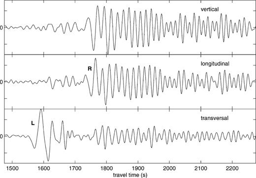
The present study will focus on Rayleigh wave fundamental mode polarisation anomalies observed at the Geoscope station PAF on the Kerguelen Isles in the southern Indian Ocean. In the period range 20 to 40 s these Rayleigh waves present significant transverse components; at 25 s period their amplitude amounts to about 55 per cent of the amplitude of the longitudinal component in some cases. As an example, the recording of event 93_216 (cfr. Table 1) in the southern part of the Java Trench, is shown in Fig. 1. The transverse component of the Rayleigh wave is easy to observe here since the station is close to a Love radiation node. Similar anomalies at the same station were reported by Maupin (1987), but the modelling tools available at that time did not allow for a discrimination between the possible causes for the transverse components.
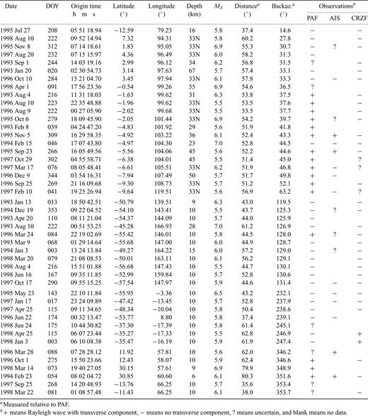
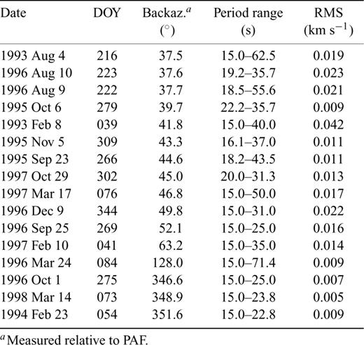
The events used in this study, listed with increasing backazimuth.
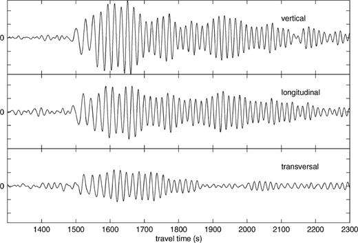
The PAF recording of event 93_216. The data have been bandpass filtered with cut-off frequencies 0.008 and 0.1 Hz, and the components are plotted with the same vertical scale.
We will first present the results of dispersion and polarisation analyses of surface wave recordings made at PAF. The observations are then compared with the results obtained from modelling surface wave propagation in 3-D models of the crust and upper-mantle beneath the Kerguelen Isles. Both isotropic and various anisotropic structures are explored. Surface waves recorded at two nearby Geoscope stations (AIS at New Amsterdam Island on the South-east Indian Ridge and CRZF at the Crozet Isles in the eastern part of the Crozet Plateau) are also analysed for comparison.
The Kerguelen Isles are located in the northern part of the Kerguelen Plateau, a large igneous province in the southern Indian Ocean. The volcanism, which has been active from 40 Ma to the present on the isles (Charvis et al. 1995), is usually considered to reflect the presence of a mantle plume in the vicinity of the islands. The polarisation anomalies reveal seismic anisotropy in the oceanic lithosphere beneath and around the plateau, a result which can be used to constrain mechanisms of lithospheric emplacement in the vicinity of oceanic plumes.
2 Data and procedures
2.1 Data selection
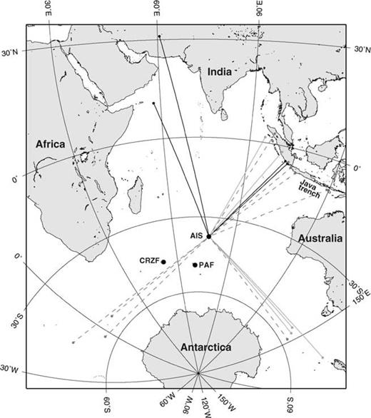
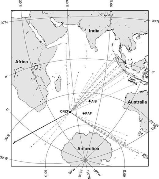
For this study we use recordings made at the three Geoscope stations PAF, AIS and CRZF of events at epicentral distances between 30° and 90°. The minimum distance was chosen to ensure that the surface wave modes are sufficiently separated in the dispersion analyses. The maximum distance merely reflects that the epicentres were chosen to be in the Indian Ocean or its immediate circumference to ensure rather uniform propagation paths, mainly in oceanic lithosphere. In order to avoid interference due to multipathing related to reflection or refraction on continental margins, the events with paths close to the African, Antarctic or Australian continents were discarded. For the surface waves to be sufficiently excited, the maximum source depth was set to 100 km and the lower MS limit to 5.5. Together these conditions imply severe restrictions on the number of events that could be used. The usually high noise level at low-latitude oceanic stations further reduced the amount of data. Consequently surface wave recordings for a total of 45 earthquakes occurring during the time period 1993 to 1998 were retained. Information about the events is listed in Table 1 and their geographical distribution is shown in Fig. 2.
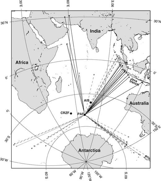
Epicentres (small, filled circles) and wave paths for the events recorded at PAF. Black line indicates observed polarisation anomaly, grey line indicates uncertain data and dashed line indicates no anomaly.
All the events were recorded at PAF, whereas 20 of them were recorded at AIS and 38 at CRZF. At PAF and, except for 1993, at CRZF, the data are from the Very Broad Band (VBB) channels with sampling rate of 20 Hz. Otherwise the data are from the Broad Band (BRB) channels with sampling rate of 5 Hz.
There are large gaps in the azimuthal distribution of the events, in particular to the south and north-west due to the proximity of the Antarctic andAfrican continents. The events selected are, roughly speaking, clustered in four groups: in the Java Trench, at the Indian–Antarctic and Macquarieridges, at the Mid-Atlantic and Atlantic–Indian ridges, and between the Indian Ocean and Iran. These groups are well separated with respect to backazimuth at PAF and it should be possible to analyse the azimuthal dependence of the polarisation anomalies.
2.2 Preprocessing
Before rotation to the longitudinal and transverse components, differences in the transfer functions for the E–W and N–S instruments have been accounted for. The gain and phase lag of the two transfer functions were calculated in the period range 20–100 s. At AIS the transfer functions were found to be equal. At the two other stations the difference in phase lag of the two components was found to be negligible (maximum difference was 0.003° at the VBB and 0.05° at the BRB channel). The gains were found to be slightly different on the two components, but their ratios were independent of frequency (maximum variation of gain ratio with period was 5 × 10⁻⁶ and 6.7 × 10⁻⁶ at the VBB and BRB channel, respectively). Thus, the difference in transfer functionscould be corrected for by simply multiplying all the samples of the E–W component by a constant value given by the ratio [Gain(N–S)/Gain(E–W)]40s at the time of the recording. These ratios vary between 0.9785 and 1.0308.
Incorrect orientation of the seismometers could also bias the estimation of polarisation anomalies. Laske (1995) evaluated the misorientation of the instruments to be between 0 and 1.5° at PAF and between 0.5 and 2° at CRZF, which is negligible in our study. Severe misorientation of the seismometers is also excluded by the fact that the polarisation of the P-phases on our seismograms is normal after rotation.
2.3 Dispersion analysis
At long periods, surface wave polarisations are usually determined by analysing the eigenvalue structure of the spectral density matrix of the three-component seismograms in a well-chosen fixed time interval (Laske et al. 1994; Park et al. 1987). In the intermediate period range of the present data, the dispersive nature of the Love and Rayleigh waves is such that they may overlap in the time domain and the standard spectral density matrix method is not well-suited, as shown by Laske et al. (1994). Instead, the Love and Rayleigh wavetrains must be separated in the time-frequency domain by moving-window analysis.
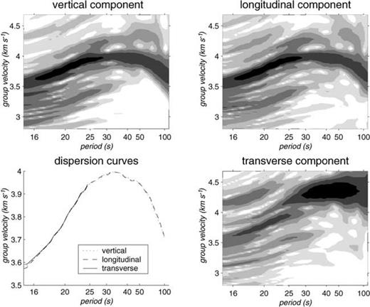
In this study, we analyse the polarisation of the fundamental mode Rayleigh wave by simply performing group velocity analysis simultaneously on the three components of the seismograms. Analysis is performed in the period range 15 to 120 s and group velocity range 2.7 to 4.6 km s−1, in order to get a complete picture of the surface waves on each component, including not only the Rayleigh wave fundamental mode, but also the overtones and Love waves. To improve the resolution of the Rayleigh wave fundamental mode group velocity curves, we perform dispersion analysis in a two-step procedure, a classical dispersion analysis followed by a residual dispersion analysis (Dziewonski et al. 1972) using the group velocity curve of the Rayleigh wave fundamental mode identified on the vertical or longitudinal component. Group velocity curves for the three components are then identified by following maxima of energy in the three time-frequency planes. An example is given in Fig. 3, which shows the results of the group velocity analysis for event 93_216, shown in Fig. 1.
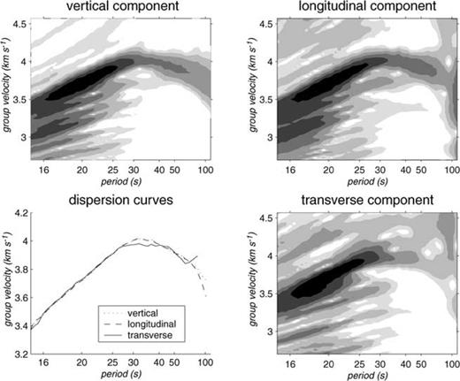
Results of dispersion analysis of event 93_216, showing the logarithm of the square root of the energy for the three components as a function of group velocity and period. The maximum energy is shown in black and the colour code changes every 6 dB from the maximum. The group velocity curves, defined by the maximum of energy at each period, are shown superimposed for the 3 components in the lower left plot.
For several of the events analysed, we observe a group velocity curve forthe transverse component which coincides almost perfectly with the group velocity curve of the Rayleigh wave fundamental mode present on the vertical and longitudinal components. In many cases, the energy along that curve is larger than the energy present at Love wave group velocities. For each event, we define the interval of coincidence between the group velocity curves for the three components as the period range over which the curves are less than 0.06 km s−1 apart. In general the distance between the curves is far less on most of the interval, as for the example in Fig. 3.
The observed group velocities are normal oceanic group velocities for fundamental mode Rayleigh waves. Although Love wave coda energy could fortuitously appear on the transverse component at the same time as the fundamental mode Rayleigh wave on the vertical and longitudinal components, the similarity of the group velocity curves on the three components over a significant interval of period and for a large number of events with different locations makes this explanation rather unlikely. Instead, we infer that we observe Rayleigh waves on the transverse component.
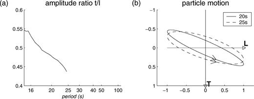
We measure amplitude and phase of the three components of the Rayleigh wave as a function of frequency in the coincidence interval by measuring amplitude and phase along the group velocity curve for each component. The transverse to longitudinal amplitude ratio and phase difference are used to analyse the amplitude of the polarisation anomaly and its ellipticity (see Fig. 4 for an example).
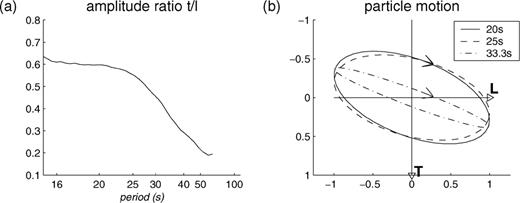
(a) Transverse to longitudinal amplitude ratio as a function of period for event 93_216, measured along the group velocity curves in Fig. 3. (b) Particle motion in the horizontal plane at three different periods derived from amplitudes and phases along the group velocity curves.
Instead of the procedure used here it would be possible, as described by Laske et al. (1994), to combine the moving-window analysis with the spectral density matrix method in order to quantify the degree of polarisation in the time-frequency plane and measure the polarisation along the curve of highest polarisation degree instead of maximum energy. The spectral density matrix method may be able to detect smaller anomalies than the simple moving-window analysis used here, where we have a rather large ‘detection’ threshold: for an anomaly to be observed the transverse to longitudinal amplitude ratio at 25 s period should be at least 0.15. This is merely due to the presence of Love waves and possible Love wave coda. In the present study, most of the polarisation anomalies are sufficiently strong to be far above the threshold value, and using spectral density matrix method would not lead to significantly different results.
3 Results of data analyses at PAF
For 16 of the 45 events analysed, the rotated seismograms at PAF and the associated dispersion diagrams present energy on the transverse component which can be interpreted as Rayleigh wave polarisation anomalies. Six events are difficult to interpret, and the remaining 23 events show no indications of Rayleigh wave polarisation anomalies. These results are summarized in Fig. 2 and in Table 1.
Table 2 gives the interval of coincidence between the dispersion curves for the three components for each of the 16 events with Rayleigh waves presenting a transverse component. Also given is the RMS error of fit between the curves for the longitudinal and the transverse components within each interval. In order to quantify the amount of energy on the transverse component, the transverse to longitudinal amplitude ratio is plotted in Fig. 5 for the 16 events within their respective interval of coincidence. At 20 s period the amplitude ratios vary between 0.3 and 0.6. For the Java Trench events there is a clear trend in the curves: the amplitude ratio decreases sharply from 20 s to 40 s period. Note that the increase of the amplitude ratio at the long period end of some curves is poorly constrained due to low amplitude Rayleigh waves at these periods, and is therefore not significant.
Intervals of coincidence and RMS errors of fit between the group velocity dispersion curves.
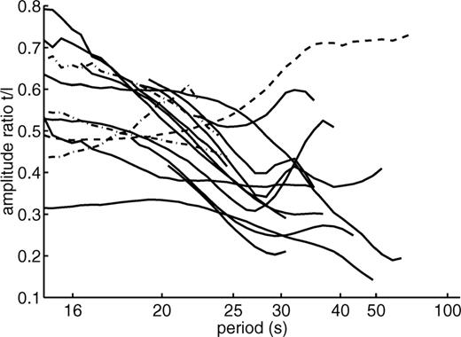
Transverse to longitudinal amplitude ratio within the intervals of coincidence for the 16 events having Rayleigh waves on the transverse component at PAF. Solid line is used for events in the Java Trench, dashed line for the event at the Indian-Antarctic Ridge, and dashed-dot line for events to the north of PAF.
In Fig. 6 the transverse to longitudinal amplituderatio at 25 s periods is plotted against backazimuth for all the 45 events. The corresponding distribution of epicentres and ray paths to PAF are shown in Fig. 2. We notice that the largest polarisation anomalies occur for events in the Java Trench with backazimuth between 37° and 64°, and to the north, at backazimuth around 350°. Polarisation anomalies are almost absent at backazimuths around 120° and 240°. We will now analyse in more detail the polarisation in the different azimuth groups.
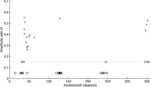
Transverse to longitudinal amplitude ratio plotted against backazimuth at PAF for all the 45 events. The squares correspond to the six uncertain events and the circles to the 23 events having no Rayleigh wave on the transverse component. Except for events 98_073 and 94_054, the ratio has been calculated at 25 s period. Due to short intervals of coincidence, the ratio has been calculated at 23.8 s for 98_073 and at 22.8 s for 94_054, and correspond to the two rightmost plus-symbols.
3.1 Java Trench
Twenty events in the Java Trench were analysed, with surface waves arriving at PAF in the backazimuth sector 27.8 to 63.2°. They separate quite clearly into two groups; the events from the northern part of the trench with backazimuth smaller than approximately 34°, showing no Rayleigh wave on the transverse component, and the 12 (of 13 altogether) events in the southern part of the trench showing a clear and strong polarisation anomaly.
A striking feature in the seismograms of 10 of the 12 events is the small Love wave amplitude, almost absent in some cases (see for example Fig. 1). This is in accordance with the focal mechanism solutions for the events, as given in the Harvard CMT catalogue. A small Love wave amplitude, and hence small Love coda, facilitates the identification of Rayleigh waves on the transverse components, which can otherwise be more difficult to discern. The events 93_244 and 98_091, located in the northern part of the trench, illustrate that problem; there are indications of weak Rayleigh waves on the transverse components, but due to the presence of moderate size Love waves, we considered that in these cases an undisputable interpretation was not warranted.
An exception in the southern part of the trench is event 94_046, which presents no transverse component although it is located in the centre of the group of events with largest polarisation anomalies. Its focal mechanism is such that it has a strong Love wave amplitude, about 40 per cent larger than the maximum Rayleigh amplitude. Nevertheless, the dispersion analysis does not show any indication of Rayleigh waves on the transverse component, as was the case for the events 93_244 and 98_091 further north in the trench. A possible explanation might be that it is suppressed by destructive interference with the Love coda.
Using the transverse to longitudinal amplitude ratio and the phase differences between the two components along the dispersion curves, the particle motion in the horizontal plane at the periods 20 s, 25 s and 33.3 s has been calculated for the events with Rayleigh waves on the transverse component. Concerning the 12 events in the Java Trench, the polarisations show three prominent features: the particle motion is elliptical, clockwise, and with the major axis oriented between the longitudinal axis and 25° away from it (measured clockwise), as shown in the example in Fig. 4. These features are independent of period, although the degree of ellipticity and orientation differ at the three periods: the major axes of the ellipses at 20 s period have a nearly constant orientation, and the degree of ellipticity decreases with increasing backazimuth. The latter also applies to the ellipses at 25 s period. At 33.3 s period the particle motion is almost linear for the first three events (i.e. backazimuth 37.6°), then becomes elliptical with minor axis equal to half the major axis at 39.7°, and thereafter the degree of ellipticity decreases gradually with increasing backazimuth.
3.2 Indian-Antarctic Ridge and Macquarie Ridge
Going southward, the next group of events analysed is located at the Indian–Antarctic and Macquarie ridges. Out of the 11 events analysed in this region, 10 have normal Rayleigh wave polarisation. However, event 96_084 is one of those with the strongest polarisation anomalies among all the events analysed in this study (cfr. Fig. 6). The anomalous energy on the transverse component correlates well with the Rayleigh waves on the longitudinal component both in time and amplitude, and the curves of maximum energy in the dispersion diagrams for the two components overlap between 15 and 71 s of period. The seismograms show simple wavetrains with no indication of multipathing or strong coda waves, and we are rather confident that the energy observed on the transverse component is indeed part of the Rayleigh wave train. We do not see any reason why this event should differ radically from the neighbouring ones; the backazimuths of the events are confined to the sector 119.5°–131.4° and thus the propagation paths are nearly coincident. The focal mechanism of event 96_084 is almost identical to those of events 98_216 and 97_290 just to the south.
The polarisation of that event in the horizontal plane is quite different from what we found for the Java Trench events. The particle motion is still elliptical, but counter-clockwise and with major axes oriented between 20° and 33° as measured counter-clockwise from the longitudinal axis.
3.3 Atlantic-Indian Ridge and Mid-Atlantic Ridge
Due to complex wavetrains arising from multipathing related to the Antarctic margin, events in the southern end of the Indian–Antarctic Ridge and in the South Sandwich Trench could not be used here, severely reducing the amount of data available in the southern azimuthal sector. Seven events with epicentres at the Atlantic–Indian Ridge and at the Mid-Atlantic Ridge have been analysed. Their backazimuth at PAF varies between 232° and 247°. Six of the seven events show no indications of polarisation anomalies. For event 98_175 the transverse to longitudinal amplitude ratio varies between 0.19 and 0.2 in the period range 15–30 s. This is slightly above the threshold value we have defined and far less than what we have found for the Java Trench events. Although Rayleigh wave polarisation anomaly can not be precluded for this event, the energy on the transverse component could also be interpreted as Love wave coda. Thus we conclude that in general the events from that region do not show clear polarisation anomalies at PAF.
3.4 North of the Kerguelen Isles
The seven events in the fourth group are more scattered geographically than those in the other groups, and are also more difficult to interpret with respect to polarisation anomalies. Event 98_073 in southern Iran is the only one which clearly has Rayleigh waves on the transverse component; both the seismograms and the dispersion analysis support unequivocally such an interpretation. For the six other events the interpretation is not straightforward. One feature these events have in common is that they have Love and Rayleigh wave amplitudes which are of the same order of magnitude. Thus, energy on the transverse component following the Love waves can be either Love coda or anomalous Rayleigh waves, or an interference between the two, and a careful analysis needs to be done in each case.
Concerning event 94_054, which is located close to event 98_073 in southern Iran, the dispersion curves for the three components coincide in the period range 15–22.8 s, compared to 15–23.8 s for event 98_073. Moreover, amplitude ratio and phase difference between the horizontal components are similar for the two events. Thus it seems likely that the energy present at Rayleigh wave group velocity is part of the Rayleigh wave train.
As an example from the source region to the north of PAF, the seismogram and the results of the dispersion analysis for event 96_275, located in the Owen fracture zone, are shown in Figs 7, 8 and 9. On the seismogram the energy following the Love waves on the transverse component correlates well with the longitudinal Rayleigh waves. There is a perfect coincidence between the dispersion curves in the period range 15–25 s for the two horizontal components. We conclude in this case that the Rayleigh waves present a transverse component.
The PAF recording of event 96_275. The data have been bandpass filtered with cut-off frequencies 0.008 and 0.08 Hz, and the components are plotted with the same vertical scale.
Same as Fig. 3, but for event 96_275.
Same as Fig. 4, but for event 96_275.
Due to short intervals of coincidence for the dispersion curves, the polarisation in the horizontal plane has been calculated at two periods only for the events 96_275 and 98_073, and at one period for 94_054. At 20 s period the particle motion is almost identical for the three events: elliptical, counter-clockwise, and with major axis between 25° and 28° from the longitudinal axis (measured clockwise). Going to slightly larger periods, the picture remains basically unchanged for events 98_073 and 96_275 (see Fig. 9).
For the events 96_088, 97_268, 98_081 and 95_208, the data do not allow of an unequivocal conclusion with respect to polarisation anomalies. We notice, however, that for events 97_268 and 98_081, located on the Central Indian Ridge, one obtains polarisation plots in the Rayleigh wave fundamental mode group velocity interval which are very similar to those obtained for the South Iranian events. Thus they support the evidences obtained from the more distant events of polarisation anomalies for Rayleigh waves propagating southwards to Kerguelen.
4 Results of data analyses at AIS and CRZF
Two other Geoscope stations, AIS and CRZF, are located close to PAF. AIS is located on New Amsterdam Island, 1413 km north-east of PAF in the direction of the Java Trench. In order to locate the cause of the polarisation anomalies at PAF, it is especially interesting to analyse the polarisation of these waves at AIS. CRZF is located 1403 km to the west of PAF, on the Crozet Isles. The geographical distribution of the events analysed at AIS and CRZF, together with the associated wavepaths, are shown in Figs 10 and 11, respectively.
Same as Fig. 2, but for the events recorded at AIS.
Same as Fig. 2, but for the events recorded at CRZF.
4.1 AIS recordings
AIS is a recent Geoscope station, with a high noise level. The amount of data available is therefore smaller than at PAF. Recordings of only 20 of the 45 events in Table 1 are available. Two of them are closer than 30°. Thus we analysed 18 events, out of which only four (94_054, 95_266, 95_309, 96_088) show clear evidences of Rayleigh wave polarisation anomalies. Five events are indeterminable with respect to Rayleigh wave polarisation anomalies due to large Love wave amplitudes. The remaining nine show no indications of polarisation anomalies.
Events 95_266 and 95_309 have epicentres in the Java Trench. The difference in azimuth at the epicentre for the great circles towards PAF and AIS is smaller than 6° for both events, showing a very good coincidence of the wavepaths to the two stations. However, the transverse to longitudinal amplitude ratio differs significantly at the two stations; at 25 s period it is 0.28 at PAF and 0.20 at AIS for event 95_266, and for event 95_309 the corresponding values are 0.37 and 0.20, respectively. Let us recall that these events have very small Love wave amplitudes, which makes it feasible to identify with good confidence weak Rayleigh waves on the transverse component.
Both events have linear or slightly elliptical, clockwise particle motion with major axes oriented between 7° and 12°, measured counter-clockwise from the longitudinal axis. These results contrast largely with those found for the same events at PAF; pronounced ellipticity and direction of major axes between 5° and 23°, measured clockwise from the longitudinal axis.
The other two events with Rayleigh wave polarisation anomalies are located to the north-west of AIS. Event 96_088 in the Owen fracture zone (Arabian Sea) clearly presents Rayleigh waves on the transverse component, the amplitude ratio being 0.34 at 25 s period. At PAF, this event is uncertain. Event 94_054 in southern Iran also seems to have a transverse Rayleigh component of the same magnitude, although it is contaminated by a high noise level on the transverse component and pronounced Love waves.
In general, the particle motion for these two events is more or less elliptical and clockwise, with major axes oriented between 16° and 20°, measured counter-clockwise from the longitudinal axis. This differs from the particle motion at PAF of event 94_054 which was elliptical and counter-clockwise at 20 s.
4.2 CRZF recordings
Of the 36 events which could be analysed at CRZF, only two exhibit evidence of Rayleigh wave polarisation anomalies. These are events 98_003 and 98_115, both located in the southern end of the Mid-Atlantic Ridge (Tristan da Cunha fracture zone). The seismograms of the two events look very much the same: small Love wave amplitudes, followed by a wave packet on the transverse component with larger amplitudes. The dispersion curves coincide in the period range 15–72.8 s for event 98_115 and between 18.4 and 40.4 s for event 98_003, the amplitude ratio at 25 s being 0.18 for both events.
At 25 and 33.3 s period the horizontal polarisation is linear and oriented between 10 and 15°, measured counter-clockwise from the longitudinal axis. At 20 s it is elliptical with counter-clockwise motion and major axis oriented as for the two other periods, though the degree of ellipticity is quite different for the two events.
Three other events, all located in the southern part of the Java Trench, present energy which could be interpreted as Rayleigh waves on the transverse component. However, the dispersion diagram for event 97_041 is complicated, and for events 97_076 and 97_302 the amplitude ratio at 25 s is less than 0.15 and can therefore not be considered as significant.
4.3 Summary of data analysis
A summary of the data analysis can be obtained by combining the maps in Figs 2, 10 and 11.
Apart from two recordings which do not fit the overall picture (one event in the southern part of the Java Trench and one at the Macquarie Ridge), Rayleigh wave polarisation anomalies are consistently observed at PAF for events in the southern Java Trench and for events located to the north. Despite quite similar wavepaths to the two stations, the Rayleigh waves generated by the events in the Java Trench show much fewer and smaller polarisation anomalies at AIS than at PAF. Two of the events located northwards present significant polarisation anomalies on the AIS recordings (versus three at PAF). At CRZF, only two events in the Tristan da Cunha fracture zone present small anomalies. This suggests that the strong transverse components observed at PAF for events located to the north and to the north-east are not a pervasive feature of Rayleigh waves in oceanic domains, but are generated by a special structure located between AIS and PAF.
The transverse components are observed at the same group velocity as the vertical and longitudinal ones. This absence of noticeable delay implies that if Rayleigh-to-Love conversion produces the transverse components, it takes place close to PAF. A conversion occurring 300 km away from the station would result in a group velocity difference between the transverse and the longitudinal components of about 0.02 km s−1, which is within the uncertainty of our group velocity measurements. A refracted Rayleigh wave may also have a transverse component. If this is the case here, the refracted wave must arrive at a large angle relative to the great circle path, and the observed group velocities also imply that the refraction must take place close to the station.
Another important result of the analysis is that the anomalous Rayleigh waves have largely elliptical particle motion in the horizontal plane, with opposite directions for the Java Trench events and those located to the north. In addition, a group of data in an intermediate backazimuth interval, generated in the northern part of the Java Trench, shows no polarisation anomalies.
Polarisation anomalies of surface waves can be caused by isotropic lateral heterogeneities or anisotropy. In the following sections we focus on the polarisation anomalies observed at PAF and quantify the possible contributions to the anomalies by different types of isotropic and anisotropic structures beneath and around the Kerguelen Isles. Concerning the anomalies observed at AIS and CRZF, the data basis is too sparse for further investigations on their origin.
5 Deviations from great circle paths in the Indian Ocean
The surface wave recordings used here have been selected in order to avoid propagation in regions which are likely to produce complex wavetrains: we have only used events situated in the Indian Ocean or its immediate vicinity, which have nearly purely oceanic paths, and propagation paths close to a continental margin have been rejected. The Indian Ocean is however a complex oceanic region with several oceanic plateaux and spreading ridges, and wavepaths may deviate from the epicentre–receiver great circles, resulting in Rayleigh waves polarised out of the great circle plane at the station. Although wave path deviations alone produce linear polarisations in the horizontal plane and will not be able to explain the ellipticity of the polarisation anomalies we observe, it is interesting to quantify their possible contribution to the anomalies.
Surface waves propagating in models with smooth, lateral variations follow rays in the horizontal plane (Woodhouse 1974). The ray tracing equations can be cast in a form which requires only a map of the phase velocity in the region of interest (Woodhouse & Wong 1986). Note that since the phase velocity distribution depends on period, different rays need to be traced for analysing the surface rays at different periods. The smallest period for which a recent phase velocity map is available for the Indian Ocean is 40 s. Surface wave data have been analysed at periods down to 20 s by Debayle & Lévêque (1997) and Lévêque et al. (1998), but with an algorithm which does not generate a phase velocity map. We will therefore first trace rays at 40 s period, and then discuss the deviations one can expect at shorter periods using indirect considerations.
Using the global phase velocity map of Trampert & Woodhouse (1997) for Rayleigh waves at 40 s period, which is an updated version of a similar map given in Trampert & Woodhouse (1995), and the exact ray calculation described in Woodhouse & Wong (1986), wavepaths were calculated for a selection of epicentres to the three Geoscope stations PAF, AIS and CRZF. The resulting angles of arrival with respect to the great circle are shown for PAF in Fig. 12 as a function of backazimuth of the great circle path at the station. The largest deviations are found for events coming from the north. The maximum deviation of −5.3° is obtained for an Iranian event, and corresponds to a transverse component equal to 9 per cent of the longitudinal one. This amplitude is smaller than the threshold of 15 per cent which we have used when analysing the data. In addition, the negative signs of the deviations for these events indicate that the wavepaths are deviated to the west of the great circle, and produce a rotation of the polarisation in the horizontal plane which is in the opposite direction to what we observe. For events in the Java Trench, where we observe the largest polarisation anomalies, the deviations predicted by the model of Trampert & Woodhouse (1997) are between 0 and 2°, produce polarisation anomalies in the opposite direction to what we observe, and well below the detection threshold. Deviations calculated at AIS and at CRZF have the same order of magnitude as at PAF.
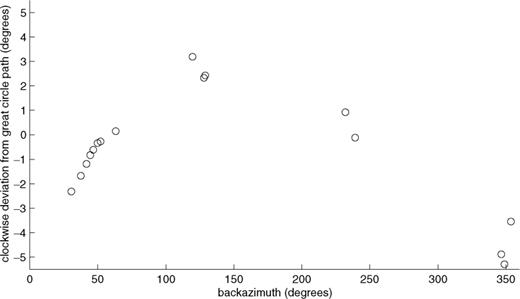
Angle of arrival of 40 s Rayleigh waves at PAF as a function of backazimuth at the station, for a representative selection of events in Table 1. The angle is measured positive clockwise with respect to the direction of the epicentre–station great circle and is calculated in the phase velocity model of Trampert & Woodhouse (1997).
At shorter periods, no phase velocity map is available. But by evaluating the mean velocity variation in the Indian Ocean, we can evaluate the amplitude of the associated path deviations. Partial derivatives show that the phase velocity of the Rayleigh waves at 20 s period are mostly sensitive to the upper 50 km of the Earth. In that depth range, the water layer and the crust are important elements and we can expect that significant phase velocity variations will be associated with variations in their thicknesses. A detailed compilation of the crustal structures in the Indian Ocean is given in Debayle (1996). Moho depth varies from about 10 km in the oceanic basins, to about 25 km under most of the oceanic plateaux. Debayle (1996) calculates the phase velocity variations associated with variations of water and crustal thickness. At 20 s period and in the region sampled by our data, the amplitude of the Rayleigh wave phase velocity variation is 6 per cent, exactly the same as the amplitude of the variation in the maps of Trampert & Woodhouse (1997) which we have used to trace the rays at 40 s period. Variations of water depth and crustal thickness can therefore be expected to produce wavepaths deviations of the order of a few degrees at 20 s period. In addition to the water and crustal thickness, variation of the mantle structure will add some variation to the phase velocity. This variation is difficult to assess directly. A tomographic study using surface waves at short and intermediate periods has recently been performed for the South-west Pacific by Pillet et al. (1999). This complex oceanic region can be expected to show velocity contrasts at least similar to the Indian Ocean in the upper 50 km. The phase variation in that region was found to be 10 per cent at 20 s period, and 6 per cent at 40 s period. We can therefore expect wave path deviations about two times larger at 20 s than at 40 s, and maximum transverse over longitudinal amplitude ratio of the order of 15 per cent.
Although they are far from negligible for the most distant events, the wave path deviations remain small compared to the polarisation anomalies we observe. This is partly related to the fact that for the relatively short epicentral distances used here, wave path deviations remain small in tomographic models of the Earth. Even when taking into account that phase velocity contrasts may be underestimated in tomographic models, deviation related to large-scale phase velocity variations can only account for a small fraction of the polarisation anomalies.
6 Wave field distortion by local structure—isotropic
The Geoscope station PAF is situated on the Kerguelen Isles, which are part of the Kerguelen Plateau, as shown in Fig. 13. In this section we examine if the observed polarisation anomalies can be explained by wavefield distortion due to the geometrical structure of the plateau in the vicinity of the station.
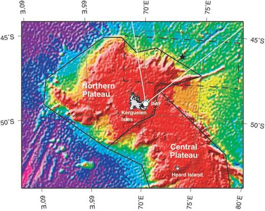
Sea floor topography of the Kerguelen Plateau. The black lines indicate the boundaries between the oceanic basins, the northern plateau and the central plateau in our models, based on those in Shipboard Scientific Party (2000). The digital bathymetry data are derived from Geosat and ERS-1 gravity information (Smith & Sandwell 1997). The black, dashed line and the two white lines indicate the location of the structure and the propagation directions in Figs 21 and 22, whereas the black star indicates the position of the plume centre in Fig. 24. See Sections 7.2 and 7.3 for further details.
6 .1Structure of the Kerguelen Plateau and surrounding basins
A recent summary on the structure and tectonic history of the Kerguelen Plateau can be found in the volume of the proceedings of the Ocean Drilling Programme devoted to the recent drilling sites on the Kerguelen Plateau and Broken Ridge (Shipboard Scientific Party 2000).
Following Könnecke et al. (1998), the Kerguelen Plateau can be divided into four domains: the northern, central and southern plateaux, and the Elan banks. The southern and central plateaux and Broken Ridge, the latter now being located ∼1800 km north-east of the Kerguelen Plateau, were formed during the Cretaceous by voluminous outpouring of magma associated with the Kerguelen hotspot. It was located below the young Indian Ocean lithosphere, at or near the ridge separating the Indian and the Antarctic–Australian plates at that time. At ∼40 Ma, the seafloor spreading between Australia and Antarctica accelerated and Broken Ridge started to separate from the plateau along the South-east Indian Ridge. At that time, the northern plateau was generated by the hotspot, located then in the vicinity of the South-east Indian Ridge. Subsequently, the Kerguelen Isles were emplaced on the northern plateau whilst the ridge migrated north-east relative to the hotspot.
The edge of the plateau, as defined in Shipboard Scientific Party (2000), has a complex shape, especially to the north-east (Fig. 13). It is surrounded by oceanic basins with age ranging from 40 My to the north-east to 80 My to the south-east (Schlich 1982). Müller et al. (1993) proposed that the hotspot is presently located beneath the western part of the northern plateau.
The crustal structure of the Kerguelen Plateau has been investigated by a series of seismic refraction profiling surveys (Charvis et al. 1995; Operto & Charvis 1996; Charvis & Operto 1999). The northernmost surveys have been done on the isles themselves, where the crust was found to be 16–20 km thick, with a very thick Layer 2 and strong velocity gradients at its base. This is similar to that found beneath intraplate islands like Hawaii (so-called ‘off-ridge setting’) and is probably representative of the structure of the whole northern plateau. A profile to the south-east of the isles, on the central plateau, shows a different type of crust: a thickness of 24 km and a particularly thick lower crust, consistent with an Icelandic-type of crust (on-ridge setting in the presence of hotspot). Low velocities at the very top of the mantle, possibly with a slightly negative gradient, were found both under the isles and under the central plateau.
We have no direct information on the seismic structure deeper in the mantle under the Kerguelen Plateau. The tomographic studies which have been done in the region do not have the lateral resolution to give a model of the mantle structure under the plateau independently of the oceanic structure around. Models based on inversion of surface waves exist however, for several relevant structures: Broken Ridge and the Ninetyeast Ridge in the northern part of the Indian Ocean (Souriau 1982) and the Ontong Java Plateau in the Pacific (Richardson et al. 2000). The mantle under Broken Ridge shows no anomaly compared to the oceanic mantle around, and the mantle under the Ninetyeast Ridge shows low velocities of 4.5 km s−1 down to about 45 km depth. Under the Ontong Java Plateau, low velocities extend much deeper, down to at least 150 km depth. The crust is also much thicker than at the Kerguelen Plateau, with an average Moho depth of 33 km.
Based on these different studies, a laterally heterogeneous model representing the lithosphere under the northern and central plateaux was constructed. It combines two velocity-depth profiles for the crust, as shown in Fig. 14. The first profile corresponds to the crustal structure found under the Kerguelen Isles, considered here to be representative of the whole northern plateau, and the other one corresponds to the crustal structure found under the central plateau (Charvis et al. 1995). The lateral extension of the structures is delimited by the edge of the plateau and the boundary between the central plateau and the northern plateau, as defined in Shipboard Scientific Party (2000). The transitions between the different structures extend laterally over 100 km wide transition zones.
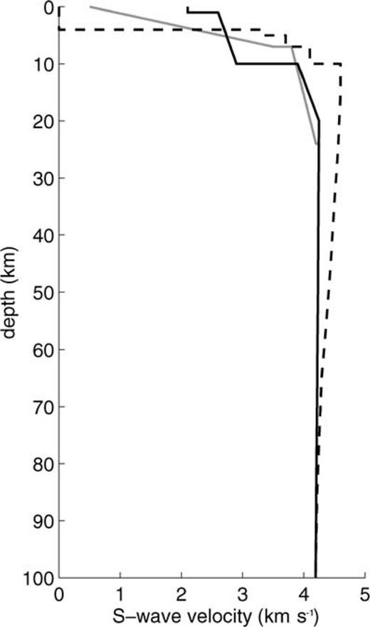
Shear-wave depth–velocity models used in this study. The solid black line is for the northern plateau, the solid grey line for the central plateau, and the dashed line for the surrounding oceanic basin.
Since we aim at evaluating the largest possible polarisation anomalies caused by refraction of waves when arriving at the plateau, we have built a model with large, although realistic, contrasts in the mantle. In our model, the mantle is characterized by low velocities extending down to 80 km depth, as shown in Fig. 14. This is similar to the mantle structure found by Souriau (1982) under the Ninetyeast Ridge, although we have used lower velocities, in agreement with the low P-wave velocities found by Charvis et al. (1995) under Kerguelen. Low velocities deeper in the mantle, as found under the Ontong Java Plateau (Richardson et al. 2000), were also tested but do not affect the results at the periods we use.
The model above is embedded in a structure representing the surrounding oceanic basins. In order to focus on waves generated by events in the Java Trench, where the largest and clearest polarisation anomalies are observed, we use an oceanic structure representative of the oceanic basin to the north-east of the plateau. Its S-wave velocity profile is shown in Fig. 14. At depths greater than 60 km, the model is a mean of four depth profiles taken at locations (49°S, 77°E),(47°S, 75°E), (45°S, 73°E) and (45°S, 71°E) in the tomographic model of Debayle & Lévêque (1997). This model is actually very similar to a mean of the two models of Nishimura & Forsyth (1989) for 4–20 My and 20–52 My old Pacific oceanic basins. Above 60 km depth, where the model of Debayle & Lévêque (1997) is not defined due to lack of resolution, we use the mean of the two models of Nishimura & Forsyth (1989), including a 6 km thick crust and a 4 km thick water layer.
6.2 Wavefield in the Kerguelen structure
The distortion of the wavefield when propagating from the oceanic basins onto the plateau has been modelled for the fundamental mode Rayleigh waves at 20, 25, 30 and 40 s period in the regional models described above. A multiple-scattering method for modelling surface wave propagation in 3-D heterogeneous structures developed by Maupin (2001) has been employed.
Results of the modelling are shown in Fig. 15 for Rayleigh waves at periods 20 and 40 s. The contours of the northern plateau and of the adjacent central plateau, as well as the location of the station PAF, are indicated. The Rayleigh waves are incident from the left, as indicated by the arrows. The structure of the Kerguelen Plateau is rotated in the horizontal plane in order to simulate a wavefield arriving at PAF with a backazimuth of 40°, similar to the waves generated by events in the Java Trench. Since it is necessary to have a denser horizontal sampling of the model at 20 s than at 40 s period, the model used at 20 s is a zoom of the model used at 40 s. Fig. 15 shows the transverse over longitudinal amplitude ratio of the wavefield at the surface. The largest amplitude ratios are observed in the vicinity of the structural boundaries; locally they reach 15 per cent at 20 s and 10 per cent at 40 s period. Away from the boundaries, the transverse component reaches only a few percent of the longitudinal one. A closer examination of the wavefield shows that the polarisation in the vicinity of PAF is slightly elliptic, with the large axis deviated clockwise with respect to the propagation direction, like on the data. Although far too small to explain the data alone, distortions related to the structure of the plateau may contribute to the observed polarisation anomalies.
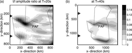
Transverse to longitudinal amplitude ratio at periods 20 (a) and 40 s (b) in our model of the Kerguelen Plateau for Rayleigh waves arriving from the Java Trench. The boundaries between the oceanic basin, the northern and central plateaux are shown by black lines. The plateaux are rotated compared to Fig. 13 such that the negative x-direction now corresponds to a backazimuth of 40° at PAF. The Rayleigh wave is incident from the left of the figure, as indicated by the arrows.
Rotating the structure in the horizontal plane to simulate surface waves coming from different backazimuths does not modify significantly the maximum or the mean amplitude ratios over the plateau.
We conclude that the structural contrasts between the Kerguelen Plateau and the surrounding oceanic basins are not sufficient to explain the strong polarisation anomalies observed at PAF.
7 Wavefield distortion by local structure—anisotropic
Surface waves can also be severely distorted by propagation through anisotropic structures (see Kirkwood & Crampin 1981, for ex.). Surface wave tomography in the Indian Ocean (e.g. Lévêque et al. 1998) and the Antarctic plate (Roult et al. 1994) reveal large-scale anisotropy in the vicinity of the Kerguelen Plateau. In addition, the proximity of the hotspot and hotspot track may have produced local anisotropic structures close to the station. The scattering scheme of Maupin (2001) used in the previous section can also handle anisotropic structures. We use it here to analyse the polarisation of Rayleigh waves propagating in various anisotropic models of the lithosphere in the vicinity of the station PAF.
7.1 Anisotropic models
As reference structure, we use a laterally homogenous model having the velocity–depth profile of the northern plateau, as shown in Fig. 14. A region containing partially oriented pyrolite is superimposed in the mantle at various depths. The isotropic mean of the structure is kept equal to the value in the reference structure. The anisotropy in the model varies from 0 to 50 per cent of the deviation of the pyrolite elastic tensor with respect to its isotropic mean. This simulates a pyrolitic mantle with 0 to 50 per cent oriented minerals. We use the elastic coefficients given by Estey & Douglas (1986) for a mantle of pyrolitic composition, with 59 per cent olivine, 12 per cent garnet and 29 per cent pyroxene. The anisotropy of the olivine crystals actually dominate the anisotropy of the pyrolite, and very similar results are obtained with models containing 30 per cent of oriented olivine crystals instead of 50 per cent pyrolite.
Pyrolite has a quasi-hexagonal orthorhombic structure with the olivine a-axis aligned with the axis of quasi-hexagonal symmetry. The symmetry axis, which also corresponds to the direction of fast P-waves, gets dominantly oriented in the flow direction of the mantle (see Mainprice et al. 2000, for a recent review on the subject), and we will interpret our results in that framework.
7.2 Wavefield in simple, anisotropic structures
The polarisation at different locations in the horizontal plane for a Rayleigh wave propagating across a rectangular structure with oriented pyrolite is shown in Fig. 16. In this case, the pyrolite symmetry axis is oriented horizontally at an azimuth of 45° relative to the propagation direction (measured clockwise). The percentage of oriented pyrolite decreases linearly from 50 per cent at Moho depth to 0 at 100 km depth. The contour of the anisotropic structure is indicated by a solid line. Before entering the structure, the Rayleigh wave has a normal polarisation, that is linear in the longitudinal direction. Propagating through the structure, it gets a small transverse component and a slightly elliptic, clockwise particle motion in the horizontal plane. The polarisation anomaly retains its amplitude after propagation through the structure, but the degree of ellipticity varies. The maximum transverse to longitudinal amplitude ratio for this model is 30 per cent.
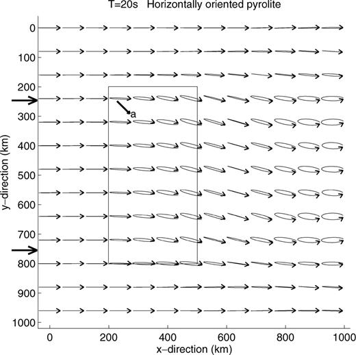
Polarisation in the horizontal plane of a 20 s Rayleigh wave propagating through an uniform, anisotropic region with horizontally oriented pyrolite. The amount of oriented pyrolite decreases linearly from 50 per cent at 20 km depth to 0 at 100 km depth. The anisotropic region is delineated by a black line. The pyrolite symmetry axis, coincident with the fast olivine a-axis, is oriented at 45° from the direction of propagation, as shown by the arrow in the anisotropic region. The Rayleigh wave is incident from the left of the figure, as indicated by the arrows.
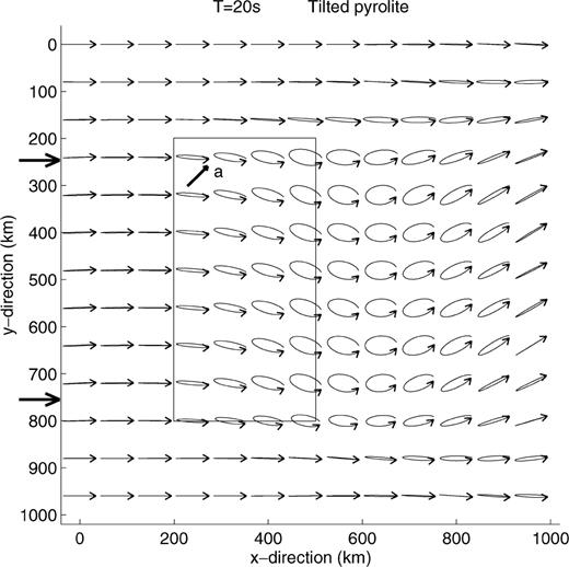
Tilting downwards the symmetry axis of the pyrolite by 45°, the polarisation anomalies get much stronger, as shown in Fig. 17. In that case, Rayleigh waves at 20 s period get a dominantly elliptical and clockwise polarisation, with an amplitude ratio between transverse and longitudinal components reaching 60 per cent. Again, the largest amplitude ratio occurs after the wave has passed the anisotropic region. We also notice that the direction of the ellipses' major axis changes considerably throughout the model.
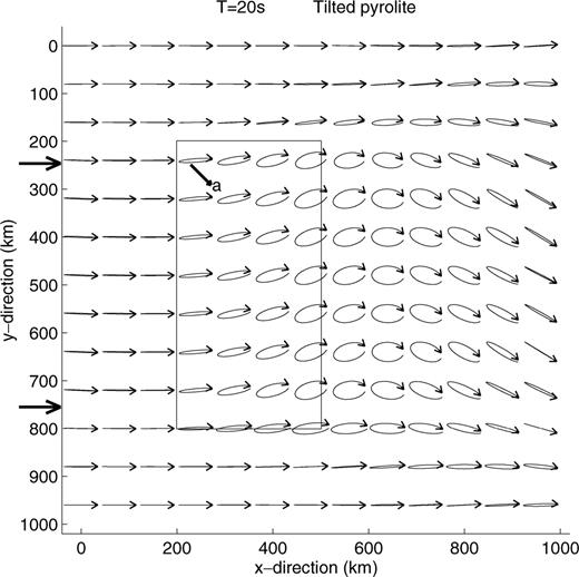
The same as Fig. 16, but the symmetry axis of the pyrolite is dipping by 45° from the horizontal plane.
At 40 s period, the polarisation anomalies are much smaller (Fig. 18) than those at 20 s period. Also the variation in the direction of the major axis is smaller. However, the particle motion is still elliptic.
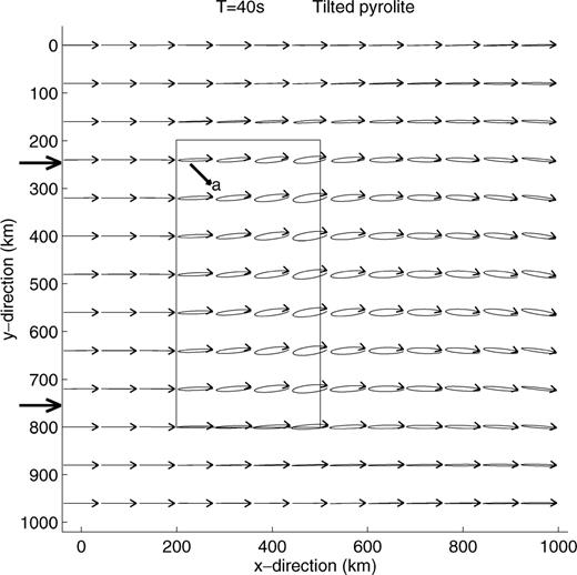
The same as Fig. 17, but at 40 s period.
The transverse over longitudinal amplitude ratio varies with the depth and the horizontal dimensions of the anisotropic structure, as shown in Fig. 19. Compared with Figs 5 and 6, which show the observed amplitude ratios at PAF, we see that the data support models with 50 per cent oriented pyrolite from Moho depth to 60 km depth, or decreasing gradually to 0 at 100 km depth, over a 300 km wide region. For a 600 km wide anisotropic region, 30 per cent oriented pyrolite from Moho to 60 km depth is sufficient, although this produces amplitude ratios which are rather large at long periods. The decrease in observed amplitude ratios with increasing period excludes models with anisotropy at the base of the lithosphere or in the asthenosphere.
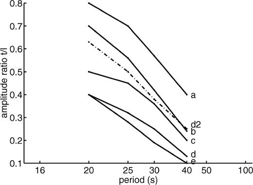
Variation with period of the transverse to longitudinal amplitude ratio in models with different depth distributions of oriented pyrolite: a: 50 per cent from 20 km to 100 km depth; b: 50 per cent from 20 km to 60 km depth; c: linear decrease from 50 per cent at 20 km depth to 0 at 100 km; d: 30 per cent from 20 to 60 km depth; e: linear decrease from 50 per cent at 20 km depth to 0 at 60 km; d2: the same as d, but for a 600 km × 600 km anisotropic region. In cases a to e, the anisotropic structure is rectangular as in Fig. 16to18. The amplitude ratio is measured to the right of the anisotropic region (at x= 700 km and y= 500 km). The orientation of the pyrolite is the same as in Figs 17 and 18.
In uniform models of anisotropy, the azimuthal variation of the polarisation anomaly is rather simple. No polarisation anomaly is observed for waves propagating in the azimuth of the pyrolite symmetry axis, but the polarisation anomaly increases rapidly when the direction of propagation deviates from that azimuth. For example, in a model such as that in Fig. 17 but with 20° azimuthal difference between the a- and x-axes, the amplitude ratio reaches 40 per cent for a symmetry axis tilting at 45°. Clockwise, elliptical motion is obtained in all cases when the azimuth of the dipping symmetry axis is positive relative to the propagation direction, as shown in Figs 16, 17 and 18, and counter-clockwise when the azimuth is negative, as shown in Fig. 20.
The same as Fig. 17, but the dipping symmetry axis has an azimuth of −45° relative to the direction of propagation.
Pyrolite in the upper mantle, with a tilted axis of symmetry, is the mechanism which—with a reasonable amount of crystal alignment—is the most efficient in producing large polarisation anomalies. The anisotropic structure should also account for the azimuthal dependence of the observed polarisation anomalies at PAF. The largest and most consistent anomalies are the strongly elliptical and clockwise polarisations of the Rayleigh waves generated by events in the Java Trench and with backazimuth between 37° and 63° (Fig. 4), whereas smaller, counter-clockwise polarisation anomalies are observed for events located to the north of PAF, with a backazimuth of 345° to 350° (Fig. 9). In between the two sectors we have a series of events at Sumatera showing no anomalies, consistent with surface waves which propagate through the anisotropic region in a direction close to the symmetry axis.
If a simple, uniform structure is responsible for the observations, the difference in particle motion for the events in the three azimuthal sectors gives a strong constraint on the possible orientation of the anisotropy. It implies that the symmetry axis of the tilted pyrolite must be oriented at an azimuth between 350° and 37°. Figs 21 and 22 show polarisation patterns at 20 s period for a rectangular model, east-west oriented and 300 km wide, with uniform anisotropy consisting of 40 per cent pyrolite at 20 km depth decreasing linearly to 0 at 100 km (50 per cent was found to give too large anomalies). The symmetry axis of the pyrolite has an azimuth of 20° and is tilted downwards by 45°. The polarization of waves arriving with a backazimuth of 350°, corresponding to waves from the Owen fracture zone and southern Iran, is shown in Fig. 21, whereas Fig. 22 shows the polarization of waves with a backazimuth of 50°, corresponding to waves from the Java Trench. We notice that the ellipses at position (x= 600 km, y= 750 km) in Fig. 21 and at (x= 800 km, y= 480 km) in Fig. 22, corresponding to approximately the same position relative to the structure, are very similar to what we have observed for events in the two azimuthal sectors. This indicates that a rather simple structure can cause the observed polarisation anomalies. Of course, these results do not preclude the possibility of more complex structures.
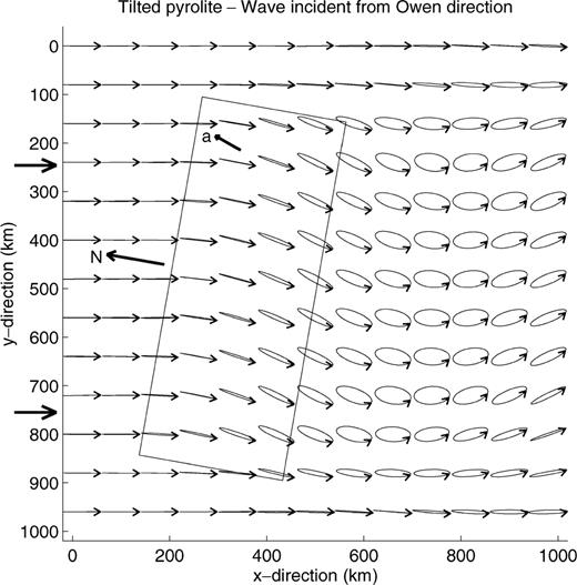
Polarisation in the horizontal plane of a 20 s Rayleigh wave propagating through an uniform, anisotropic region with oriented pyrolite. The amount of pyrolite decreases linearly from 40 per cent at 20 km depth to 0 at 100 km depth, its symmetry axis is dipping by 45° from the horizontal plane, and the azimuth relative to north is 20°. The azimuth (relative to north) of the propagation direction is 170°, corresponding to a backazimuth of 350°.
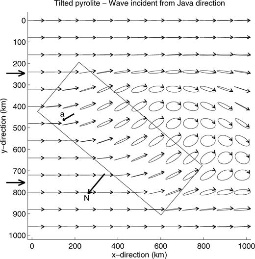
The same structure as in Fig. 21, but here the azimuth of the propagation direction is 230°, corresponding to a backazimuth of 50°.
Besides, a comparison of the orientations of the ellipses large axes in Figs 21 and 22 with the observations, suggests that PAF is not situated in the anisotropic region, but to the south of it. This is also consistent with the fact that polarisation anomalies are not observed for surface waves coming from south-east and south-west. The distance between PAF and the anisotropic region is however limited by the fact that the transverse components arrive at the same time as the longitudinal and vertical ones. Conversion of Rayleigh to Love waves by a distant anisotropic structure would generate transverse phases arriving earlier than the main Rayleigh phase, as pointed out in Section 4.3.
Combining this information, we conclude that a region with a 300 km north-south extension, located north and north-east of the Kerguelen Isles, with dipping pyrolite at an azimuth of about 20°, would explain well the data set. The east-west extension of the anisotropic region is not well constrained by the data, but it has to be large enough to be sampled by surface waves coming from the Owen Fracture zone and from the Java Trench. The region is indicated by a dashed, black line on the map in Fig. 13, where ray paths with backazimuths 350° and 50° are shown as white lines.
7.3 Wavefield in a plume-like, anisotropic structure
Following the track of the Kerguelen hotspot as proposed by Müller et al. (1993), the hotspot was located north of the Kerguelen Isles at Cretaceous time. It is therefore interesting to study the polarisation of Rayleigh waves in models where the orientation of the minerals follows the pattern expected for plume-like structures. We construct a very simple model of a plume following the same principles as Rümpker & Silver (2000). A vertical slice showing the orientation of the minerals as a function of depth is given in Fig. 23. The depth of the anisotropy is dictated by the variation of polarisation anomalies with period in our data, not by geodynamic constraints. In the horizontal plane, the model is axisymmetric, and has 50 per cent oriented pyrolite at Moho depth.
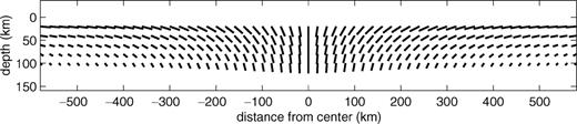
Vertical cross-section showing the orientation of pyrolite in the plume model. The length of the bars is proportional to the percentage of oriented pyrolite, which is equal to 50 per cent in the plane at 20 km depth, and along the symmetry axis of the plume.
The polarisation of the Rayleigh waves at 20 s period in that model is shown in Fig. 24. Waves which propagate through the centre of the plume, indicated by the star, show very little polarisation anomalies. The largest anomalies are strongly elliptical and occur in two 300 km wide zones away from the plume centre. We notice that the polarisation varies rapidly in the horizontal plane. Waves which have travelled to the left of the plume centre are polarised clockwise, whereas those which have travelled to the right of it are polarised counter-clockwise. A plume of the type described here located to the north-north-east of the Kerguelen Isles (centre position is indicated by the black star in Fig. 13), such that events from Java propagate on one side of the plume centre, those from Sumatra, which show no polarisation anomaly, propagate through it, and those from the north propagate on the other side, explains also quite well the observations at PAF.
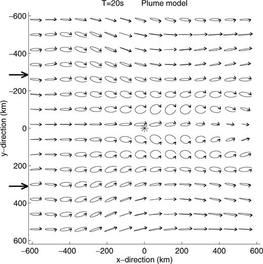
Polarisation in the horizontal plane of a 20 s Rayleigh wave propagating through the plume model. The location of the plume symmetry axis is indicated by a star.
8 Discussion
Analysis of Rayleigh waves in the period range 20 to 50 s at three nearby Geoscope stations in the Indian Ocean reveals that the waves have very strong polarisation anomalies for some wavepaths. Waves arriving at the station PAF, on the Kerguelen Isles, from north-north-west and north-east have transverse components with an amplitude of up to 55 per cent of the longitudinal ones at 25 s period. Some polarisation anomalies are also observed at AIS, although smaller and for a few events only.
We show that deviation of the wave path from the epicentre-to-station great circle, or distortion of the wavefield when it propagates from the oceanic basins onto the Kerguelen Plateau, are not sufficient to explain the observations at PAF. Anisotropy, on the other hand, is able to produce polarisation anomalies similar to those observed. We show, for example, that a 300 km wide uniform, anisotropic region containing 40 per cent oriented pyrolite (equivalent to 24 per cent oriented olivine), situated to the north of Kerguelen, can explain the data quite well, provided the olivine a-axis is tilted downwards from the horizontal plane by about 45°. The anisotropy has to be situated at the top of the mantle in order to match the decrease of the polarisation anomaly with increasing period. Our preferred model has a linear decrease of anisotropy from Moho to 100 km depth. In order to match the amplitude and the ellipticity of the observed polarisations, the symmetry axis of the pyrolite, which coincides with the fast axis of the olivine crystals, should be tilted downwards away from Kerguelen at an azimuth of about 20°. We show that the tilted pyrolite could also be part of an axisymmetric structure similar to a plume.
In the simulations we have performed, the structure around the anisotropic region is isotropic. Let us note however that similar results would be obtained if it was replaced by an anisotropic structure, for example with horizontally oriented olivine crystals, in which Rayleigh and Love waves show almost normal polarisations. The variation in olivine orientation from regionally horizontal to tilted in the vicinity of Kerguelen would then produce the polarisation anomalies.
Our preferred model produces only a small anisotropy in Rayleigh wave phase velocity, about 2 per cent at 20 s and 1 per cent at 40 s, with the fast axis in the direction of the pyrolite symmetry axis. Surface wave phase velocity studies of the Indian Ocean (Lévêque et al. 1998) and of the Antarctic plate (Roult et al. 1994) show anisotropy in the vicinity of Kerguelen. Roult et al. (1994) find 4 per cent anisotropy in Rayleigh wave phase velocity at 76 and 143 s period at the Kerguelen Isles, with a fast axis oriented at an azimuth of 40°. In their model, the anisotropy has a maximum at PAF, where it is two times larger than 500 km away. Lévêque et al. (1998) also find anisotropy, with a fast axis oriented at an azimuth of about 70° in the vicinity of Kerguelen, but with a smaller amplitude: 1 per cent anisotropy at 100 km depth and 2 to 3 per cent at 50 km depth. Notice that olivine or pyrolite oriented between 40 and 70°, as suggested by the tomographic studies, is not well-suited to explain our polarisation data since the particle motion for events in the Java Trench would then be almost normal, or the same as for the events in Iran. These studies use longer periods than we do, and do not have the resolution needed to detect a 300 km wide structure located under the Moho. The discrepancy in orientation between tomographic studies and this study most likely reflects the difference between the regional orientation in the Indian Ocean seen by the phase velocities, and a local structure associated with the plateau or the Kerguelen hotspot and revealed by the polarisation anomalies.
No anisotropy was detected beneath any of the three Geoscope stations PAF, AIS or CRZF by Barruol & Hoffmann (1999) when analysing SKS-splitting. And no crustal or mantle P-wave anisotropy is apparent either in the results of the seismic surveys conducted in northern Kerguelen by Charvis et al. (1995). This confirms that the anisotropic region is not located beneath the Kerguelen Isles. 40 per cent oriented pyrolite with a symmetry axis dipping at 45° produces 2 per cent P-wave anisotropy in the horizontal plane, with the fast P-wave direction aligned with the pyrolite symmetry axis. The P-wave anisotropy in the horizontal plane would be larger for horizontally oriented pyrolite, reaching 6 per cent. This is similar to the amount of anisotropy found at Moho depth under the southern Kerguelen Plateau (Operto & Charvis 1996) and confirms indirectly that our estimate of 40 per cent oriented pyrolite is a realistic amount of anisotropy in a local structure.
In the southern plateau, the fast axis is oriented along the plateau. Operto & Charvis (1996) interpret this anisotropy as resulting from the stretching of a continental fragment detached from the Australian–Antarctic margin during a jump of the South-east Indian Ridge early in its history. The tectonic context is therefore very different from the northern plateau, which is believed to be of purely oceanic origin (Charvis & Operto 1999, for ex.) and is close to the present location of the hotspot.
The most direct information we have on the mantle under Kerguelen comes from mineralogical studies of xenoliths collected on the Kerguelen Isles (Mattelli et al. 1996, in particular). They suggest that the mantle under the isles is the result of intense partial melting which occurred during the last of the three episodes of intense volcanism associated with the Kerguelen hotspot. This episode, dated ∼40 Ma, also created the northern part of the Kerguelen Plateau (Charvis et al. 1995; Mattelli et al. 1996). At that time, the hotspot was still located in the vicinity of the South-east Indian Ridge, from which it started to separate shortly afterwards. During this episode, the mantle may have been stretched in the direction of the expansion, possibly in relation to the detachment of the hotspot from the ridge. It may however, have been too warm to be able to imprint anisotropic structures.
Alternatively, anisotropy in the lithosphere over a hotspot could arise from strong olivine crystal alignment in residual dunites, as proposed by Levin & Park (1998) for explaining anisotropy in the lithosphere under Hawaii. Although dunite can be strongly anisotropic, it is unlikely to be able to explain a significant large-scale anisotropy since it is thought to emplace in the conduits by which basaltic melts migrate upwards through the lithosphere, and constitutes therefore only a minor part of the lithosphere under the hotspot. In addition, the mantle xenoliths collected at Kerguelen, in particular the dunite xenoliths, do not show foliation or lineation (Mattelli et al. 1996; Gregoire et al. 1997).
Yale & Phipps Morgan (1998) argue for a very strong hotspot-to-ridge flow in the asthenosphere from the Kerguelen hotspot to the South-east Indian Ridge. This flow would be located between Kerguelen and New Amsterdam, that is in the region where we localize an anisotropic structure, but deeper in the mantle. A strong non-uniform flow at depth may induce non-horizontal stretching of the lithosphere above, resulting in tilted orientation of the minerals.
A complex pattern of mantle anisotropy in the 300 to 500 km vicinity of the Hawaii hotspot has also been reported by Levin & Park (1998), who studied Love waves. Oblique orientations of olivine has been proposed as an explanation of Love wave polarisation anomalies in association with subduction zones (Brisbourne et al. 1999) and the Tibetan Plateau (Yu et al. 1995), and may be a rather common feature of the mantle.
A natural extension of this study would be to analyse if the Love waves also present polarisation anomalies at PAF, and if they are consistent with the Rayleigh mode ones. Since the fundamental mode Love wave overlap with the Love and Rayleigh overtones, a complete modelling of the whole wave train is necessary to analyse Love wave polarisation anomalies in the appropriate period range.
The polarisation anomalies we observe decrease with increasing period. Extrapolating to longer periods, we can however expect that in some places the large axis of the particle motion of the Rayleigh waves might deviate from the direction of wave propagation by several degrees. This is of the same order of magnitude as the polarisation anomalies, interpreted as wave path deviations, used by Laske (1995) and Laske & Masters (1998) to improve the resolution of tomographic studies. Laske & Masters (1998) show that wave path deviations have the potential to improve the lateral resolution of the global anisotropic structure of the mantle, but that they yield puzzling results in some cases, for example at the Geoscope station KIP at Hawaii. This may indicate that a combined interpretation of the measurements in terms of wave path deviations and polarisation anomalies would be more appropriate in some cases.
This study shows that Rayleigh wave polarisation anomalies can be sufficiently strong to be detectable. They provide unique information on the orientation of mantle anisotropy. Important constraints on the model can be obtained with only one station. But the numerical modelling we present also shows that the polarisation anomalies vary rapidly laterally, showing the potential of analysing polarisation anomalies at a network of stations.
Acknowledgments
Many thanks to the Geoscope management group for making their high quality data easily accessible. Thanks also to Magali Billien for calculating the deviations from great circle path propagation. The dispersion analysis was performed using a code written by M. Cara, D. Rouland and J.-J. Lévêque. E. Debayle provided a model of the Indian Ocean. Comments by S. Operto and an anonymous reviewer helped improve the manuscript. The maps were prepared with GMT software (Wessel & Smith 1991).
References
