Composition and microstructure of magma bodies from effective medium theory

Summary

1 Introduction

Understanding the microstructure and composition of magma bodies such as magma chambers beneath volcanoes and beneath mid-ocean ridges is important for exploring how melt is being delivered from the mantle and the propensity for the magma to erupt (e.g. Zollo et al. 1996; Singh et al. 1998). Seismic inversion techniques provide us with information concerning the wave velocity, attenuation and anisotropy through a medium. Interpreting this information in terms of the underlying stratigraphy requires knowledge of the physical properties, such as the bulk and shear moduli, and the microstructure of media through which the waves travel. Although magma chambers are complex, one important structural feature affecting seismic wave propagation is the proportion of the body that is fully molten and the interconnected and complex nature of the fluid and any solid components. Here we do not attempt to model the individual contribution of each of the phases. Instead, we start with separate fluid and solid phases with known physical properties, and use effective medium theory to explore how varying the concentration and physical microstructure of the combination of the phases affects the elastic stiffness and hence the wave velocity and the anisotropy of the resulting effective media.

2 Effective medium theory

The principal tool in our analysis here is that of effective medium theory, to represent the overall behaviour of a body as a propagating seismic wave ‘sees’ it, and thus to avoid having to specifically model the details of small-scale microstructure for which we have very few constraints. There have been quite a number of attempts to make quantitative estimates of how composite material properties vary with composition, which broadly fall into two groups. There are those that take an essentially statistical approach and give upper and lower limits on the values, such as Hashin–Shtrikman and Voigt–Reuss bounds (Hashin & Shtrikman 1963; Reuss 1929), but these are of little use for making quantitative estimates in practice as the bounds are so far apart. The other general approach is to make a simplifying assumption concerning some aspect of the geometry or microstructure, such as a specific type of inclusion geometry, which is what we do here. There are two principal existing theories on ways to implement this to encompass the entire range of phase concentrations, both of which start from the analytic solution for the elastic deformation arising from the addition of a single inclusion in an infinite medium (Eshelby 1957).

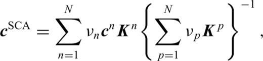
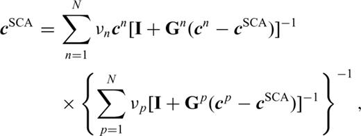
The first theory is the self-consistent approximation (SCA). This method, pioneered by Budiansky (1965), Hill (1965) and Wu (1966), uses the solution for a single inclusion and approximates the interaction of many inclusions by replacing the background medium with that of the yet-to-be-determined effective medium. For any proportion of two different phases it gives explicit expressions for the resulting elastic moduli, which are coupled and must be solved by simultaneous iteration (see the Appendix). This method has the advantage of being simple to compute, but one drawback lies in the interpretation of the microstructure. That is for two phases, e.g. a fluid phase added to a solid background matrix, the fluid inclusions are isolated below 40 per cent fluid content, and the solid and fluid phases can only be considered to be mutually fully interconnected between 40–60 per cent. For our application to magma bodies we would expect such interconnection at much lower melt fractions.

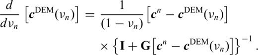
The second is differential effective medium (DEM) theory. This models a two-phase composite by incrementally adding inclusions of one phase to a background matrix of the other and then recomputing the new effective background material at each increment (Boucher 1976; McLaughlin 1977; Cleary et al. 1980; Norris 1985, see Appendix). The incremental approach allows the calculations at any composition irrespective of starting concentrations of original phases. This method is also implemented numerically and addresses the drawback of the SCA in that either phase can be fully interconnected at any concentration. However, the very aspect of the method that permits this brings with it the disadvantage that the starting microstructure essentially pre-determines the final matrix-inclusion structure.

A far more detailed account of these two methods and their differences is given in Mainprice (1997) and Jakobsen et al. (2000), the latter also containing a derivation of the explicit expressions for their implementation. We attempt to take advantages of both of these methods and minimize their shortcomings by using a combined effective medium method (Sheng 1990; Hornby 1994; Jakobsen et al. 2000), a combination of the SCA and DEM theory. Specifically, we use the formulation originally written by Hornby (1994) for examining shales, and subsequently developed by Jakobsen et al. (2000) for gas hydrates. Used on its own, the DEM theory can be used to calculate the stiffness matrix for a composite whose microstructure comprises a background ‘host’ phase containing inclusions of the second (fluid or solid) at any composition. At first, the SCA can be used to calculate the stiffness matrix for a bi-connected two-phase material at a given concentration of fluid (in the 40–60 per cent range) and then the DEM procedure can be used to incrementally calculate the desired final composition that may be at any concentration.

The inclusions are introduced in the form of oblate spheroids with semi-axes a and c (for Cartesian coordinates x₁, x₂ and x₃, x²₁/a²+x²₂/a²+x²₃/c²= 1; x₁, x₂≤a, x₃≤c, Fig. 1). The existence of an analytic solution for a spheroidal inclusion (Eshelby 1957) and the fact that the shape of the spheroid can be defined by a single parameter, the ratio of its semi-axes a/c, make this choice of geometry advantageous. The inclusions can be introduced in an aligned manner (where they all lie parallel, with their c-axis parallel to the vertical, 3 direction), in which case the material is transversely anisotropic with the 1 and 2 directions being equivalent (Fig. 1). Alternatively, they can be introduced in a randomly oriented, averaged fashion in which case the resulting material is isotropic. The motivation behind examining the case of aligned inclusions is to gain an insight into some of the affects that might arise from rocks with a strong crystal preferred orientation (e.g. Boudier & Nicolas 1995) and melt films that form in foliation or veins within the rock texture, exhibiting a preferred orientation. A prevailing overall direction for the background stress field can also result in an anisotropic material, even if the inclusions are randomly aligned, through opening and closure of inclusions not aligned with the direction of principal stress. The isotropic case is examined in order to gain some understanding of composites that are predominantly melt-based and therefore have no anisotropy, or where compositional- or temperature-driven convection in the melt means that even if the melt tends to crystallize with a preferred direction, the result is isotropic. It also provides a good reference model for the anisotropic case.

Figure 1

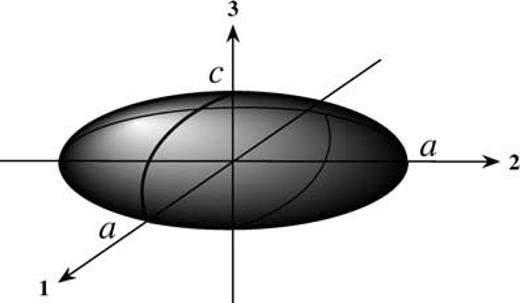
Schematic diagram illustrating the oblate spheroidal shape of the inclusions considered here. Note that it has a circular cross-section in the 1–2 plane, and a is greater than or equal to c for the inclusions considered here.

Open in new tabDownload slide

In order to produce models of composites appropriate to the magma bodies we are interested in investigating, we take the elastic parameters for our starting molten and solid phases from the observed velocity and density for melt and surrounding rock from the magma chamber along part of the East Pacific Rise (Singh et al. 1998). The P- and S-wave velocities and density of the melt are 3.3 and 0 km s⁻¹ and 2600 kg m⁻³, respectively, and for the surrounding rock are 6.0 and 3.2 km s⁻¹ and 2700 kg m⁻³ respectively. The choice of starting materials can be easily tailored to the specific rheology of the region being examined. We present here results for three distinct microstructures; isolated solid crystal inclusions suspended in melt, isolated melt inclusions in a solid background matrix, and a fully bi-connected melt and solid composite, where both phases are fully interconnected throughout. In addition, we demonstrate the effect of a range of aspect ratios of the inclusions of either melt or solid, and of introducing the inclusions in an aligned or randomly oriented fashion.

3 Results

3.1 Microstructure

Fig. 2 illustrates the effect of the geometry of the microstructure of a two-phase melt and solid matrix composite on the P- (Fig. 2A) and S-wave (Fig. 2B) velocities for the entire range of compositions. In order to highlight just the effect of the microstructure, both the starting phases are isotropic and the inclusions are introduced as spheres. The resulting composite is thus also isotropic, irrespective of the microstructure. The short-dashed lines show the P- and S-wave velocities calculated using DEM theory resulting from starting with 100 per cent melt and progressively replacing it with isolated inclusions of solid, crystalline material. In this case the melt is connected but the solid inclusions are isolated. Such a condition may arise when magma is cooled very slowly in a convective environment. The most dramatic feature of these curves is that both the P- and S-wave velocities remain much lower than for other microstructures considered until the melt fraction is reduced to almost zero, whereupon the velocity increases rapidly to match that of the pure solid. The bold, solid lines show the velocities resulting from the opposite process of starting with a solid background matrix and adding melt inclusions. In this case the solid matrix is connected and the melt inclusions are not connected. Such a situation may arise at the initial phase of melting of rocks. Here the velocities decrease monotonically from that of the solid matrix to that of the melt, and for any given melt fraction this microstructure results in the highest velocity. The third set of lines shows the effect of using the SCA to calculate the stiffnesses (and hence velocities) for composites of 45, 50 and 55 per cent melt (medium-dashed, narrow-solid and long-dashed lines, respectively) and then, using these as starting points, using DEM theory to add or subtract material to explore the behaviour for the full range of compositions from pure solid to pure melt. In this case, both solid and melt phases are connected. In a magma reservoir at ocean spreading centres, where a magma chamber may be in a steady state, both phases might be connected at a large range of melt fractions. Predictably, both the P- and S-wave starting velocities decrease as the starting melt fraction increases, i.e. the initial velocities are progressively lower for 45, 50 and 55 per cent melt. The microstructure resulting from these starting points then dictates that for any given melt fraction, the velocities for the resulting composite are lower for the higher initial melt fractions.

Figure 2

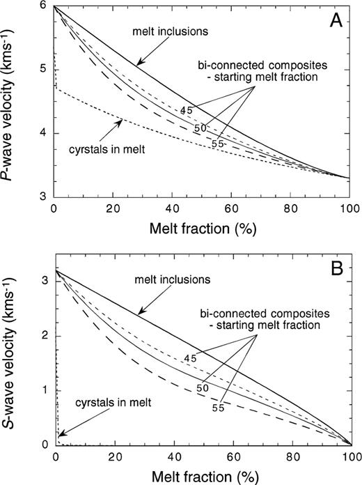
Variation of (A) P- and (B) S-wave velocities with melt fraction for spherical inclusions and different microstructures: isolated solid crystals suspended in melt (short-dashed line), solid matrix with isolated inclusions of melt (bold-solid line) and a fully bi-connected melt–solid composite starting from initial compositions of 45, 50 and 55 per cent melt (medium-dashed, narrow-solid and long-dashed lines, respectively).

Open in new tabDownload slide

3.2 Aspect ratio

Fig. 3 shows the effect of introducing inclusions of melt into a solid background matrix with aspect ratios other than 1 (spheres) on the P- (Fig. 3A) and S-wave (Fig. 3B) velocities. The inclusions are introduced aligned with their c-axis parallel to the 3 direction, so although the starting materials are isotropic, the resulting composite is transversely isotropic with stiffnesses (and hence velocities) varying out of the 1–2 plane. The P-wave velocity in the 1–2 plane (‘horizontal’, bold-dashed lines) is greater than that in the 3 direction (‘vertical’, narrow-solid and narrow-dashed lines) for any given melt fraction, and this discrepancy increases with increasing aspect ratio, i.e. the difference between horizontal and vertical velocities is greater for a/c= 100 than for a/c= 10, which is greater than for a/c= 1 (where it is zero). Small departures from spherical inclusions have the most marked effect and beyond a/c∼ 10, very little change in the velocity, in either direction, is induced by further increasing the aspect ratio. The effect on the S-wave velocity is similar in that, for a given melt fraction, the in-plane horizontal S-wave velocity is greater than the vertical S-wave velocity. However, whereas increasing the aspect ratio beyond ∼100 produces very little change in the horizontal velocity, the vertical velocity continues to drop off more dramatically at low melt fractions with increasing aspect ratio. For a/c= 100, a melt fraction of only 20 per cent is sufficient to reduce the vertical S-wave velocity to ∼15 per cent of the value for the solid matrix.

Figure 3

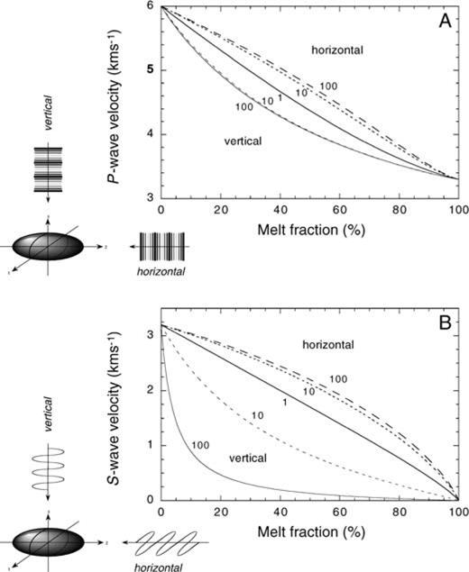
Variation of (A) P- and (B) S-wave velocities with melt fraction for inclusions of aspect ratios a/c= 1 (spheres), 10 and 100 (thin discs) aligned with their c-axis in the 3 direction. The microstructure is that of melt added to a background solid matrix. Numbers along curves indicate aspect ratios. For anisotropic materials (a/c= 10 and 100), ‘horizontal’ (bold-dashed lines) and ‘vertical’ (narrow-solid and narrow-dashed lines) velocities are plotted. The sense of P- and S-wave directions and polarization, and the alignment of inclusions are indicated by the schematic diagram in the bottom left-hand corner.

Open in new tabDownload slide

3.3 Orientation of inclusions

Introducing spherical inclusions is not the only way to maintain an isotropic composite. The other aspect of the geometry of the microstructure we consider is that of an isotropic composite with randomly oriented spheroidal inclusions. We compare this with one where the inclusions are aligned along a particular direction, as might result from a preferential direction of growth or prevailing overall stress state. Fig. 4 illustrates how the P- and S-wave velocities compare for the isotropic composite (solid lines) with randomly oriented inclusions against the individual horizontal (short-dashed lines) and vertical (long-dashed lines) velocities in the transversely isotropic material with aligned inclusions. In the case shown here the aspect ratio of the inclusions is 10, and inclusions of melt are added to a solid background matrix. Calculations of the effect of solid crystals in melt or a bi-connected composite produce lower velocities than plotted here for any given melt fraction, as shown in Fig. 2. As expected, the P- and S-wave velocities through the isotropic composite lie between the extremes of the horizontal and vertical velocities resulting from the aligned inclusions. However, it is not a simple arithmetic average, and it is particularly noticeable around 50 per cent melt fraction that the P-wave velocity for the isotropic material is closer to the P-wave velocity in the vertical direction for the transversely isotopic case. Conversely, the S-wave velocity in the isotropic material is closer to the S-wave velocity in the horizontal direction than the vertical direction in the anisotropic material.

Figure 4

P- and S-wave velocity variations with melt fraction for inclusions of aspect ratio a/c= 10 both aligned with their c-axis in the 3 direction (anisotropic, vertical and horizontal velocities plotted) and randomly oriented (isotropic). The microstructure is that of a melt added to a background solid matrix.

Open in new tabDownload slide

3.4 Anisotropy

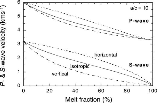
Calculation of the directional dependence of velocity in the composites also allows us to examine the anisotropy exhibited. Here we define the anisotropy as the difference between the vertical and horizontal velocities, normalized by the velocity of the pure solid matrix. Fig. 5 shows the P- and S-wave anisotropy for a range of aspect ratios and microstructures. The bold lines show the anisotropy resulting from adding melt inclusions of aspect ratios 10 (solid) and 100 (dashed) to the solid background. The narrow lines show the anisotropy resulting from starting with a fully bi-connected solid–fluid composite and adding or subtracting melt inclusions of aspect ratios 10 and 100. The anisotropy from starting from a pure melt and adding crystal inclusions is not plotted as it is zero for all but the tiniest melt fractions as the velocity in both the horizontal and vertical directions remains almost that of a pure melt (Fig. 2). The anisotropy is zero at both 0 and 100 per cent melt as the individual solid and melt phases are isotropic.

Figure 5

Variation of (A) P-wave anisotropy ([V_Pvert−V_Phoriz]/V_P0) and (B) S-wave anisotropy with melt fraction for different aspect ratios (a/c= 10, solid lines, and 100, dashed lines), and for isolated melt with different microstructures inclusions in a solid matrix (bold lines) and a fully bi-connected melt–solid composite (narrow lines).

Open in new tabDownload slide

When starting from the solid background, the magnitude of the P-wave anisotropy is greatest at ∼30–35 per cent of the melt fraction, whereas when starting with the bi-connected composite at 50 per cent melt the P-wave anisotropy is most pronounced around 20 per cent (Fig. 5A) of melt. For low melt fractions there appears to be little difference in the P-wave anisotropy induced either by the geometry of the microstructure or the aspect ratio. However, above about 15 per cent melt fraction, the composite formed by adding melt inclusions to the solid background results in significantly greater P-wave anisotropy than the bi-connected material.

For S-wave anisotropy, the aspect ratio of the inclusions has a much more marked effect than for P-wave anisotropy for the equivalent melt fraction and microstructure. When starting from a solid background, the S-wave anisotropy is greatest at ∼30 and 10 per cent of melt fractions and for a bi-connected composite at ∼10 and 2 per cent, for a/c= 10 and 100, respectively (Fig. 5B). In further contrast to the trends in variation of P-wave anisotropy, the S-wave anisotropy is greater for higher aspect ratios for almost all melt fractions, irrespective of the microstructure.

4 Discussion and Conclusions

4.1 Microstructure

The assumed underlying connectivity of the microstructure has a fundamental effect on the resulting velocities (Fig. 2). The physical interpretation of the change in microstructure resulting from the DEM calculations is that the original connectivity and geometry is maintained even though the proportions of the constituent phases may change. This is illustrated most dramatically by the very low P- and S-wave velocities for the composites starting from pure melt (short-dashed lines, Fig. 2). As more and more solid crystal inclusions are added, although they form a greater volume fraction of the composite they remain isolated in the surrounding melt and so contribute almost nothing to the shear strength and very little to the bulk modulus, hence the near zero S-wave velocity and the very low P-wave velocity. In direct contrast, the opposite process of starting with a solid background and introducing inclusions of melt (bold-solid lines, Fig. 2) maintains a rigid and connected matrix within which the melt is isolated, so it retains some shear strength (and hence finite S-wave velocity) right up until it becomes pure melt. Similarly, the bulk modulus (and hence P-wave velocity) is much higher than for the alternative considered microstructures. Using the SCA to give a bi-connected starting composite thus forms the intermediate case where the solid phase forms a rigid structure to support both shear and compressional stresses at all melt fractions and the corresponding P- and S-wave velocities are higher than for the melt starting case. However, the melt also forms interconnected pathways between the matrix and so weakens the structure compared with that of a matrix with isolated inclusions. The three starting compositions for the bi-connected structures shown here of 45, 50 and 55 per cent melt (medium-dashed, narrow-solid and long-dashed lines) have progressively less interconnected matrix and more fluid, which is seen in the trend of lower starting P- and S-wave velocities with increasing melt fraction for these cases.

Another diagnostic of the effect of the microstructure is observed in the second derivative of the S-wave velocity with respect to melt fraction (Fig. 2B), i.e. the change of the slope of the velocity curve with melt. For both the pure melt and pure matrix starting points, the rate of change is almost zero with the gradient remaining roughly constant and only increasing and decreasing rapidly at very low and high melt fractions, respectively, as the other added phase finally dominates. This is due, again, to the fact that the DEM calculations inherently preserve the original microstructure and so it is the background phase, be it melt or solid, that dominates the physical properties of the composite even when there is a greater volume fraction of the second phase. However, when the starting composite comprises bi-connected melt and solid, adding or removing either melt or solid immediately affects the physical properties because whichever is being added or removed is always part of the connected microstructure of pathways through the material that transfer stress through the structure.

It is noteworthy that because the density of the assumed solid and melt phases are so similar (difference < 4 per cent) most of the observed variation in velocity is derived purely from the change in the corresponding components of the stiffness matrix. The fact that there is a significant departure from the initial P- and S-wave velocities after the addition/removal of only a few per cent of melt for all the microstructures shown here again demonstrates the important effect that compositional variation has on seismic observables.

4.2 Aspect ratio

When the inclusions introduced are oblate (a/c > 1) they naturally introduce anisotropy into the composite, as shown for inclusions of melt of aspect ratios 10 and 100 in Fig. 3. Intuitively, the spheroids offer more resistance to compression in the 1 and 2 directions than in the 3 direction (see schematic figure, bottom left Fig. 3A) and hence, for a given melt fraction, the P-wave velocity is greater in the horizontal direction than in the vertical one. The stiffness, and hence velocity for spherical inclusions lies between these bounds. Above aspect ratios of ∼10, the change in elastic properties induced by increasing the aspect ratio is minimal. This is useful for minimizing the range of melt fractions that are consistent with a given velocity, but has the disadvantage of making it hard to tie down the exact geometry of any inclusion-type microstructure. The number of variables is reduced by the fact that there are only two distinct velocities when considering propagation along the 3 direction or in the 1–2 plane. The velocities of both the horizontally and vertically polarized waves in the 3 direction and the shear wave travelling in the 1–2 plane with a component in the 3 direction are identical. The remaining distinct velocity is that of the shear wave travelling and polarized in the 1–2 plane. The S-wave directional dependence is much greater than that of the P waves, as the fluid inclusions offer much less resistance to shear in the out-of-isotropic 1–3 or 2–3 planes (i.e. for vertically propagating waves of any polarization, see the schematic in Fig. 3B) than in the isotropic 1–2 plane (i.e. for horizontally propagating waves polarized in the 1–2 plane).

Hence not only is the difference in velocity relative to spherical inclusions much greater in the vertical direction than in the horizontal one, but the effect of aspect ratio continues to be very pronounced even for very high aspect ratios (a/c > 100, equivalent to long thin discs). This illustrates one example of where using more than one observable can provide tighter constraints on the model. For instance, if both P- and S-wave velocities have been obtained in a region where one suspects that a melt exists in isolated pockets that have a preferred orientation or alignment, the P-wave velocity, which is insensitive to the aspect ratio, can be used to tie down the melt fraction from reading off the corresponding value from Fig. 3(A). The plot for S-wave velocity (Fig. 3B), which is sensitive to the aspect ratio but not the melt fraction can then be used to constrain the aspect ratio, which is consistent with the observed S-wave velocity and the melt fraction implied from the P-wave velocity.

4.3 Orientation of inclusions

The way in which the aspect ratio of the inclusions affects the microstructure is shown in Fig. 4, where the resulting P- and S-wave velocities are compared for aligned and randomly oriented inclusions with a/c= 10. The curves for the individual horizontal and vertical P- and S-wave velocities are the same as those for a/c= 10 in Figs 3(A) and (B), respectively. Although the randomly oriented inclusions constitute an isotropic composite, the inclusions are, on average, weaker or less stiff than spheres as is illustrated by a comparison with the velocities for spherical inclusions from Fig. 3. Thus, even when modelling a region or composite that is isotropic, one still has to consider details of the microstructure such as the aspect ratio as there are differences on the small scale that are capable of producing globally isotropic media with different seismic velocities.

Although a certain amount of information regarding the anisotropy introduced by considering a preferential direction of alignment of melt inclusions can be gleaned from Figs 3 and 4, Fig. 5 illustrates more explicitly the variation of P- and S-wave anisotropy with melt fraction for both a solid background matrix and a fully interconnected fluid–solid composite, for aspect ratios of 10 and 100. For P-wave anisotropy, at low melt fractions the microstructure of both the solid background matrix and the bi-connected composite is dominated by the connectivity of the solid phase and whether the fluid exists as isolated inclusions or with some connectivity between them makes very little difference. However, above around 10 per cent melt, the solid background matrix exhibits a greater magnitude of anisotropy than for the bi-connected composite. This is because where the melt inclusions are isolated, there is a much greater contrast in rigidity between the 1 or 2 and the 3 direction and there is no space for the trapped fluid to go to release the induced pressure gradient from the P wave. Where the inclusions form a connected phase, melt can re-distribute itself within the composite to alleviate some of the applied stress and so the contrast in stiffness between the directions for the fluid-filled oblate spheroids is reduced. As seen from Fig. 3(A), the effect of increasing the aspect ratio from 10 to 100 on P-wave velocity through the solid matrix with melt inclusions is fairly small. The same is seen to be true here for the bi-connected composite, and the anisotropy is comparable for aspect ratios of 10 and 100 at all melt fractions. However, the S-wave anisotropy is dramatically affected by increasing the aspect ratio (Figs 3A and 5B). The inability of fluid to support shear stress results in the directional dependence of the S-wave velocity being very sensitive to both the aspect ratio and the microstructure. This provides another useful means of delineating between competing parameters in models for a given velocity structure.

4.4 Application to magma bodies

The main purpose of this approach, and the plots presented here, is to provide a diagnostic tool in making quantitative statements concerning the composition and detailed structure of magma chambers underlying volcanoes or along mid-ocean ridges. The starting point is the result of a seismic survey, or other geophysical data, that can be inverted for the velocity structure of the region. Then, by making some simplifying assumptions regarding the properties of the constituent phases that might be present, such as liquid magma, the P- and S-wave velocities and any directional dependence data can be used in conjunction with the plots to narrow down the likely structure and composition. This will aid a fuller understanding of the dynamics of any evolution of the magma body, which is important in assessing the likelihood of eruption. Mainprice (1997) notes that only a few per cent of a second phase introduced in inclusions is sufficient to overwrite any anisotropy of the starting phase. This is important as it means that the results are not very sensitive to the assumed individual starting materials, which adds confidence to the robustness of this method.

As an example of how to proceed, consider the results of the inversion from a hypothetical 3-D seismic survey that show a clear low-velocity zone about 1–2 km below the surface of a volcano. If the S-wave velocity is zero, or very close to it, then we can conclude (from Fig. 2B) that the chamber is predominantly melt, although some fraction of it may exist in a crystalline phase. From Fig. 2(A) we can project the known P-wave velocity to obtain an estimate of the melt fraction. Any error or uncertainty in the P-wave velocity can also be mapped directly into an uncertainty in the melt fraction simply from this plot, although unfortunately owing to the shallow slope of the curve at high melt fractions, small errors in velocity translate into relatively large errors in the composition. If the S-wave velocity is non-zero then there are a greater range of possibilities. Again, the S-wave velocity is a useful starting point as it is much higher for melt inclusions in a background solid matrix than for a bi-connected composite for any given melt fraction, and so combined with the P-wave velocity should at least give a range of possible melt fractions and microstructures that are consistent with both. Then, by examining any P-wave anisotropy (Fig. 5(A)), one can differentiate between strongly anisotropic microstructures (e.g. aligned inclusions) and isotropic ones (e.g. spherical inclusions or randomly aligned oblate spheroids). For a region that exhibits anisotropy, Fig. 5B is particularly useful as it illustrates the strong S-wave velocity dependence on the aspect ratio. For the case of melt inclusions in a solid background matrix, we have extended the effective medium theory method to calculate the attenuation owing to melt being driven through the composite in response to the seismically induced pressure gradients (Singh et al. 2000). For this case, the addition of measurements of attenuation would provide a further constraint on the composition and microstructure.

The procedures and results presented here provide a relatively straightforward way of translating velocity models of regions containing magmatic bodies into quantitative maps of the composition and microstructure and fabric of the underlying rheology. This should greatly improve our ability to interpret the state and evolution of the magma chambers and, in particular, provide a way to further quantify the risk of future eruption.

Acknowledgments

This research is a part of TOMOVES project funded by the European Commission. SCS was supported by a UK NERC Senior Research Fellowship. The authors are grateful for many fruitful discussions with John Hudson on effective medium theory.

Appendix

2010 Self-consistent effective medium (SCA) theory

In this approach the elastic field for each inclusion is determined approximately using a single inclusion placed in a host having the elastic properties of the effective medium. The approximation will give estimates for isotropic composites which lie within the Hashin–Shtrikman bounds at all concentrations. If ν_n is the fractional volume of the nth constituent such that ∑_n=1^Nν_n= 1, then the stiffness tensor can be written as

(A1)

where K is a tensor and depends on the solution for c^SCA. This expression can be solved iteratively, by setting an initial value for c^SCA, computing K, and then re-evaluating c^SCA. This tensor can be computed analytically for a spheroidal inclusion in a host matrix, resulting in

(A2)

where Gⁿ is the Green's tensor for the nth element.

Differential effective medium (DEM) theory

Suppose we know the elastic properties of the overall material at a certain value of ν_n of the concentration of one of the constituents and we wish to predict the effective properties at higher concentrations. The effective properties are computed at other values of ν_n by successive operations of removing an infinitesimal subvolume of the nth component. At each successive increment of component n, the composite at the previous step is taken as the host material. It is important to note that, in order to increase the concentration of the nth component ν_n by Δν_n, a concentration Δν_n/(1 −ν_n) of the composite material must be replaced. If the concentration of material with stiffness cⁿ is ν_n in a composite of effective property of material s(ν_n) and Δν_n is added to the composite by replacing the same amount, then the effective property of the final media can be computed using

(A3)

where Kⁿ is computed for the included material cⁿ in the effective material with elastic stiffness c(ν_n+Δν_n). By inserting the value of the K tensor, we can obtain the DEM equation for anisotropic composite

(A4)

These expressions can be solved using numerical integration techniques, such as the Runge–Kutta method. Note that the DEM formulae are not symmetrical in the constituents. For a two-component solid a different material is created if the roles of host and included materials are interchanged. If the solid material is the host material, then the DEM provides a composite material where the solid is connected and the other material, which could be a fluid, is not connected, and the reverse is true if fluid is the host and the solid is the inclusion. If the composite of interest contains more than two constituents (as is likely to be the case for most rocks), one can extend the DEM to include such materials (see Jakobsen et al. 2000). The essential difference between the SCA and DEM is that the result for the DEM depends on the path taken, i.e. the order in which the constituents are added to the composite. In other words, if a constituent is not connected before invoking the DEM, then that constituent will never become connected at any concentration of included material. However, if the constituent is already connected before invoking the DEM, then that constituent will remain connected with subsequent changes in the concentration of that constituent. For two components to be connected, it is important to start the DEM procedure with a composite material where both constituents are connected, and this is the approach used here. We use the SCA to obtain a biconnected material, and then use the DEM.

References