


SUMMARY
By integrating the truncated complex scalar gravitational motion equations for an anelastic, rotating, slightly elliptical earth, the complex frequency-dependent earth transfer functions are computed directly. Unlike the conventional method, the contributions of both oceanic load and current to all nutation periods, as well as the atmospheric contributions to prograde annual, retrograde annual and retrograde semi-annual nutation, are included in the integration via outer surface boundary conditions, all of which are expanded to second order in ellipticity. A modified ellipticity profile of second-order accuracy for the non-hydrostatic earth is obtained from Clairaut's equation and the PREM earth model by adjusting both the ellipticity of the core–mantle boundary and the global dynamical ellipticity to modern observations. The effects of different earth models, anelastic models and ocean models are computed and compared. Finally, a complete new nutation series of 343 periods, including in-phase and out-of-phase parts of longitude and obliquity terms, for a more realistic earth is obtained and compared with other available nutation series and observations.
1 Introduction
Precession and nutation, as well as three other earth rotation parameters (polar motion [two parameters] and universal time), are very important parameters in linking between the terrestrial reference frame (TRF) and the celestial reference frame (CRF). Rigid-earth precession–nutation models have been improved such that they are now very accurate; models include SMART97 of Bretagnon (1998) , REN2000 of Souchay (1999) and RDAN97 of Roosbeek & Dehant (1998). However, an acceptable geophysical nutation theory for a non-rigid earth with oceans and atmosphere, including all known effects at the 0.1 milliarcsecond level, is not yet available and requires further study (Dehant 1999 ).
Usually, the methodology of non-rigid earth nutation study falls into four categories: (1) completely fitted from modern observation, very long baseline interferometry (VLBI) plus lunar laser ranging (LLR) (see Mccarthy 1996 and Shirai & Fukushima 2000); (2) semi-analytical methods (Mathews 1991 , 2000); (3) based on the Hamiltonian theory and variational principles, an analytical method extends the method of rigid earth nutation study to the study of non-rigid earth nutation (Getino & Ferrá, ndiz 1991, 1999); and (4) purely geophysical approaches, in which the so-called non-rigid earth nutation transfer function is integrated from the equations of earth deformation by normal mode expansion and the direct numerical integration method (Wahr 1981a; Dehant & Defraigne 1997; Schastok 1997; Huang 1999), which is used in this study.
2 The numerical integration method
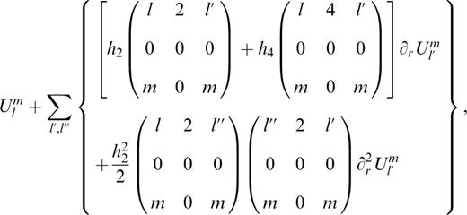
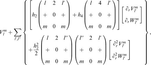
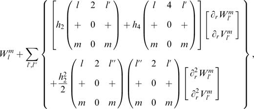
Smith (1974) developed an algorithm in which the tensor elastodynamic equations of infinitesimal motion, that is, the Lagrangian and Poisson equations, are transformed from the elliptical domain to an equivalent spherical domain (ESD), and all the vector and tensor equations are then converted to scalar equations using the generalized surface spherical harmonics (GSSH) expansion. Using the symmetry restrictions in the ℛe space, appropriate linear combinations of poloidal and toroidal vector fields are deduced and are used to define disjoint spaces of vector-valued functions that completely contain various sets of eigenfunctions. The scalar ordinary equations—coupled due to the ellipticity—as well as a set of boundary conditions governing the elastic gravitational normal modes of a rotating, slightly elliptical earth in hydrostatic equilibrium, which has an isotropic elastic constitutive relation, are finally derived, truncated to finite order and described in computable forms, on which almost all the modern nutation and tide theories of a non-rigid earth (Wahr 1981a; Dehant & Defraigne 1997; Schastok 1997; Huang 1999) are based.
The given equations of motion are in ordinary differential form. Due to the resonance effect in the integration of the frequency-dependent transfer functions of the earth nutation from a rigid earth to a non-rigid earth, the uncertainty of the nutation terms will be amplified. This is particularly true for those frequencies in the vicinity of the free core nutation (FCN), whose period is about one sidereal day in the TRF and about 432 sidereal days in the CRF. In order to overcome the resonance ‘pollution’ and to detect small signals such as the contributions of atmosphere and oceanic current, Schastok (1997) and Huang (1999) re-derived the boundary conditions on the stress tensor and gravitational potential field to second order in ellipticity, instead of to first order as given by Smith (1974), as well as the boundary conditions for the displacement field (Huang 1999, 2001), i.e. the following quantities should be continuous across any welded boundary between two solid regions:
and the following scalar quantity in ordinary differential form should be continuous across any boundary:
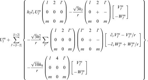
The notation is the same as in Smith (1974), that is, U, V and W are the poloidal radial component, poloidal tangential component and toroidal tangential component of the displacement vector respectively, l and m are the degree and order of their GSSH, ∂r is the partial derivative of the radius r, and h2 and h4 are the second- and fourth-order coefficients (at the earth mean surface, r=a) of the Legendre expression of h (see Moritz 1990), which is the radial displacement of the equidensity surface from its mean spherical surface.
The 3×3 parenthesis

named the J-square symbol (Smith 1974), can be expressed as a product of two Wigner 3-J symbols of quantum mechanics. The components of the J-square symbol are limited by

2.1 The contributions of the ocean and atmosphere
In the conventional method, the contributions of the oceanic load and current are calculated by the angular momentum method (or torque method) and added ex post facto into the nutation series for an earth without an ocean layer. In this study, these effects, as well as the contributions of atmospheric relative motions, are included directly in the integration of the equations of earth deformation via a non-free outer surface boundary condition.
If the earth does not include ocean and atmosphere, the outer surface of the solid earth is a free one, that is, the pressure and the stress tensor at the outer boundary of the solid earth cancel in the integration. On the other hand, if the ocean and/or atmosphere are included in the earth system, the outer surface of the solid earth is no longer a free one. The stress tensor at the outer boundary of the solid earth is given by Sasao & Wahr (1981) in tensor form and expanded into scalar form of three components (Plm, Qlm, Rlm) to second order in ellipticity ( Huang 2001, with some corrections to the errata in Schastok 1997):
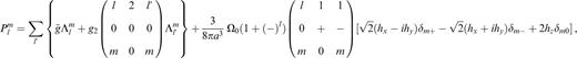
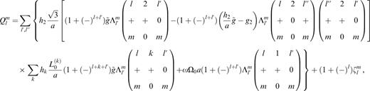
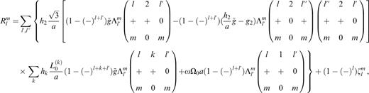
where ζ is the contribution of the relative angular momentum (of oceanic current or wind), i.e. h(hx, hy, hz),
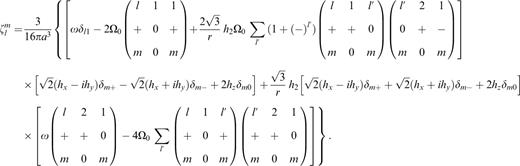
In these expressions of the continuity quantity at a non-free outer surface boundary, there are two quantities related to the oceanic and atmospheric contributions, h(a, Ω) and Λlm(a, Ω), which represent the relative angular momentum and the load respectively, where a and Ω denote the mean radius of the earth and the circular frequency of the nutation. g˜ and g2 are the mean gravity (without the centrifugal part) and the latitude-dependent part of the gravity at the earth's surface respectively, Ω and Ω0 are the nutation circular frequency and the mean angular velocity of the earth rotation respectively, δ is the Kronecker symbol and Li(j)=
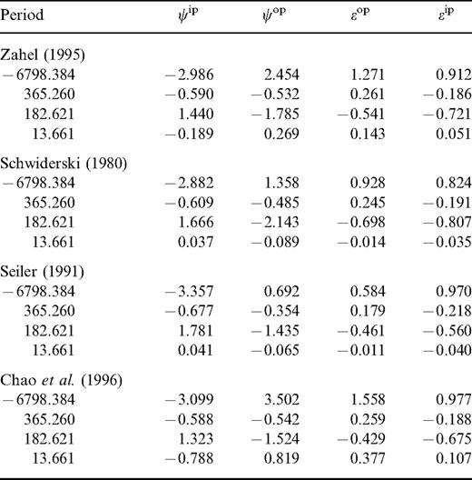
There are several ocean models available (Schwiderski 1980; Seiler 1991; Zahel 1995; Chao 1996; Gross 1995) that give both amplitudes and phases of several dominant diurnal tides (e.g. K1, P1, O1, Q1) of the load and the relative motion (current) separately. The model of Zahel (1995) is adopted in this work. For other diurnal frequencies, we adopt the resonance admittance formula of Wahr & Sasao (1981, p. 754, eq. 4.8 or A5) for the tide height t21. As for the R-factor in eq. (4.8) of Wahr & Sasao (1981), the formulae for Love numbers were given in Wahr (1981b, p. 697, eq. 4.18) and Wahr & Sasao (1981, p. 749, eqs 2.6–2.8), and the Love numbers of the reference frequency (O1 tide) were given in Wahr (1981b, p. 699, Table 6, for 1066A), but the FCN resonance period is changed from 460 days to 432.8 days in this paper. For the D-factor in eq. (4.8) of Wahr & Sasao (1981), we use a slope linear function to interpolate and extrapolate other diurnal frequencies among O1, P1, and K1.
Comparison of the four main nutation terms (units: mas).
The atmospheric spectrogram, however, is usually strongly contaminated and there is no atmosphere model that can give the amplitude and the phase of the diurnal atmospheric tides, and it is not easy to build the corresponding relation between the atmosphere and the nutation in the frequency domain. Nevertheless, the atmosphere has an obvious character, that is, it is influenced mainly by the sun. Due to the earth's revolution, the major variation of atmospheric angular momentum is of annual period, which is the dominant source of the excitation to the annual variation of the earth's polar motion, but it does not effect the diurnal nutation. Meanwhile, because of the earth's rotation, there should also be a signal of near-diurnal variation in the atmosphere spectrum that will contribute to the diurnal nutation.
In this paper, we adopt the concept of celestial effective angular momentum (CEAM) in the frequency domain. The EAM in TRF, χ , can be converted pointwise to the CRF, χ′, by multiplying by a factor of the sidereal rotation, eiΦ (or eiΩt). The CEAM is defined as ( Brzezinski 1994)

where Φ is the temporal Greenwich sidereal time.
The original near-diurnal variation signals in the TRF become low-frequency signals in the CRF; on the other hand, the original long-period signals in TRF become high-frequency signals in the space. We can then use a low-pass filter to keep the low-frequency signals of χ′ and filter out the high-frequency part easily ( Bizouard 1998 ). Huang (2000) processed the atmospheric EAM data during 1980.0 and 2000.0 provided by the National Center for Environmental Prediction (NCEP) Maryland, USA, in which there are four even points at 00.00, 06.00, 12.00 and 18.00 hr GMT every day. In that study, the upper limit of the integration for the wind field is 10 mbar, and the oceanic reaction to the atmosphere is hypothesized to be a non-inverted barometer (NIB) because it is more likely for the high-frequency variation. The amplitudes of the long trend and three periods from standard least-squares fits, as well as the corresponding relative angular momentum, h, caused by the wind are given in that paper and are used in this study.
2.2 Inelastic mantle
If the mantle inelasticity is considered, the Lamé coefficients become frequency-dependent complex and will produce an out-of-phase nutation part (Dehant 1987). A frequency-to-the-power-α model ( Anderson & Minster 1979) is used to compute these Lamé coefficients in this study. The radially dependent quality factor, Q, is taken from the anelasticity model QMU of Sailor & Dziewonski (1978), and the reference frequency Ω0 and the power α are taken as 200 s and 0.15 respectively ( Wahr & Bergen 1986).
2.3 The ellipticity profiles of the earth's interior
In addition to the density profile, the ellipticity profiles of the earth's interior are very important for the nutation computation, although they are less well known. The precession is mainly related to the global dynamical ellipticity of the earth, H, while the FCN, which is a very important normal mode in the earth nutation, is related to the ellipticity of the core–mantle boundary (CMB), εCMB.
The ellipticity profiles of the earth's interior are dependent on the density profile and can be obtained from the second-order Clairaut equation for an earth in hydrostatic equilibrium, which is plotted as a solid line in Fig. 1. High-precision astronomical observations have shown that both H and εCMB from the PREM ( Dziewonski & Anderson 1981) earth model, which is a hydrostatic equilibrium model, are obviously inconsistent with the observations. It is usually believed that the deviation of the earth's interior from hydrostatic equilibrium is a good interpretation.
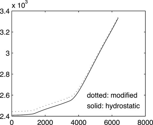
Ellipticity profile of the earth for equipotential surfaces.
In order to be compatible with the latest observations, we assume that the CMB and two discontinuities (r=5701 and 5971 km) are in non-hydrostatic equilibrium, subject to two constraints: (1) the resultant H should be consistent with the observed value, i.e. Hobs≈0.00327379, while from PREM, HPREM≈0.003240; and (2) the resultant retrograde FCN period (real part) should be −432.8 sidereal days (with ocean), while it is about −458 days for PREM. The former constrained FCN period ignores the electromagnetic and topographical coupling at the CMB. Mathews (2000) showed that the electromagnetic coupling at the CMB can play an important role in the FCN. In order to satisfy the second requirement, εCMB is modified from 0.002547 (for PREM) to 0.002666, which is an increase of 4.7 per cent (if the electromagnetic coupling at the CMB is accounted for, it is enough to increase it by 3.5 per cent; Mathews 2000 ). Based on these two constraints, we can obtain a new equipotential ellipticity profile from the Clairaut equation and the PREM density profile that differs a little from that derived from the earth that is internally in fully hydrostatic equilibrium everywhere. For example, εICB, εr=5701 km and εr=5971 km are changed to 0.002454, 0.003200 and 0.003224, increasing from their equilibrium values by 1.4, 2.3 and 1.2 per cent, respectively. The resultant modified ellipticity profiles of the equipotential surfaces can then be obtained from the Clairaut equation and are also plotted in Fig. 1 (dotted line).
As a result of the expressions up to second order in the boundary conditions, we are able to obtain the period of the prograde free inner core nutation (FICN), which is +465.6 sidereal days (with ocean) for the modified ellipticity profile and +470.6 sidereal days for an earth in hydrostatic equilibrium.
3 Results and comparison
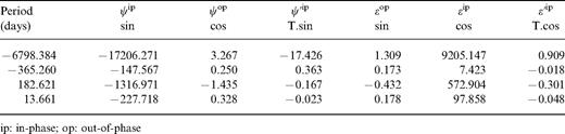
By integrating the truncated complex scalar gravitational motion equations, the complex earth transfer functions for each nutation frequency are computed directly and are then convolved with the rigid earth nutation series REN2000. In the integration, the density profile of the earth model PREM is used in this study, and the normal step length of the integration is 5 km. The resultant non-rigid earth nutation series are truncated at 5 µas, and 343 terms (of periods from 6798.384 to 4.003 days) are finally kept, in which the effects of the oceanic load and current and atmospheric wind are included; these are listed in Table 1 (the full table is available in the online version of the journal at www.blackwell-synergy.com). For convenience we list the four main terms here.
The final non-rigid Earth nutation series (units: day, mas, mas yr−1). The reference frame is ecliptic and equinox of date (J2000.0).
3.1 The contribution of ocean and atmosphere
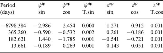
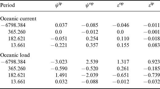
The total oceanic contributions to nutation of all 343 frequencies are given in Table 2 (the full table is available in the online version of the journal at www.blackwell-synergy.com), in which the Zahel (1995) model is used. The four main terms are listed here for convenience. The contributions of the oceanic load and relative angular momentum to the four main nutation terms are presented in Table 3. From Tables 2 and 3, the contribution of the oceanic current to the annual term is small, but it is large to the semi-annual and 13.66-day terms. The contribution of the oceanic load to all the in-phase/out-of-phase parts of the longitude/obliquity part of the 18.6-yr, annual and semi-annual terms is at the milliarcsecond level.
The total contribution of oceanic load and current to the Earth nutation (units: days, mas or mas cy−1). The reference frame is ecliptic and equinox of date (J2000.0).
The contribution of oceanic load and current to four main nutation terms (units: days and mas).
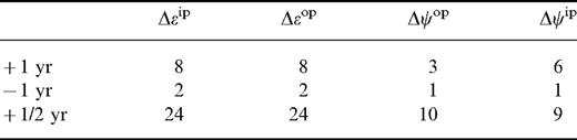
In order to compare the differences among the different ocean models, their contributions to the four main nutations are calculated and listed in Table 4. It can be seen from Table 4 that the differences among the various ocean models are still large; most of them are larger than 0.1 mas, especially the difference for the ψop18.6 yr term, which can reach 1 mas. Their differences for the annual term are less than 0.1 mas. The contributions of the atmosphere wind for annual and semi-annual nutation are small (<0.03 mas) and are given in Table 5.
The oceanic contribution to four main nutation terms by various ocean models (units: days and mas).
The contribution of the atmospheric wind to the annual and semi-annual nutation (unit: µas).
3.2 Comparison
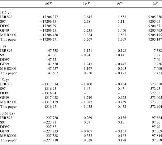
The four main nutation terms of this work, in which the contributions of ocean and atmosphere have been corrected, are compared with other available observational and theoretical series (see Table 6), namely (1) the IERS Conventions ( McCarthy 1996) nutation series (IERS96) fitted from VLBI observations by Dr T. Herring, (2) the Dehant & Defraigne (1997) model (DD97), (3) the Schastok (1997) model (S97), (4) the Getino & Ferrándiz (1999) series (GF99), and (5) the Mathews (2000) model (MHB2000).
Most of these terms from the various models are compatible with each other at the 0.1 mas level, although the models used different methods (wholly fitted from observation, semi-analytical, numerical integration or analytical), but the δΨop of the 18.6-yr and annual terms still show a large discrepancy. This may be a result of electromagnetic, topographical and/or gravitational dissipation at the CMB and the dissipation of the FCN and requires further study.
Acknowledgments
We are indebted to Drs J. Schastok and V. Dehant for their kind help, encouragement and careful reviews. Another anonymous reviewer is also thanked for constructive suggestions. This work was partly supported by the Project NSFC 10073015, the Major Project of CAS KJ951-1-304 and NSFC 19833030 and the project of the Open Laboratory of Dynamic Geodesy (CAS) L99-(10).
References
