


Summary
The Strait of Georgia is a topographic depression straddling the boundary between the Insular and Coast belts in southwestern British Columbia. Two shallow earthquakes located within the strait (M = 4.6 in 1997 and M = 5.0 in 1975) and felt throughout the Vancouver area illustrate the seismic potential of this region. As part of the 1998 Seismic Hazards Investigation of Puget Sound (SHIPS) experiment, seismic instruments were placed in and around the Strait of Georgia to record shots from a marine source within the strait. We apply a tomographic inversion procedure to first-arrival traveltime data to derive a minimum-structure 3-D P-wave velocity model for the upper crust to about 13 km depth. We also present a 2-D velocity model for a profile orientated across the Strait of Georgia derived using a minimum-parameter traveltime inversion approach.
This paper represents the first detailed look at crustal velocity variations within the major Cretaceous to Cenozoic Georgia Basin, which underlies the Strait of Georgia. The 3-D velocity model clearly delineates the structure of the Georgia Basin. Taking the 6 km s−1 isovelocity contour to represent the top of the underlying basement, the basin thickens from between 2 and 4 km in the northwestern half of the strait to between 8 and 9 km at the southeastern end of the study region. Basin velocities in the northeastern half are 4.5–6 km s−1 and primarily represent the Upper Cretaceous Nanaimo Group. Velocities to the south are lower (3–6 km s−1) because of the additional presence of the overlying Tertiary Huntingdon Formation and more recent sediments, including glacial and modern Fraser River deposits. In contrast to the relatively smoothly varying velocity structure of the basin, velocities of the basement rocks, which comprise primarily Palaeozoic to Jurassic rocks of the Wrangellia Terrane and possibly Jurassic to mid-Cretaceous granitic rocks of the Coast Belt, show significantly more structure, probably an indication of the varying basement rock lithologies. The 2-D velocity model more clearly reveals the velocity layering associated with the recent sediments, Huntingdon Formation and Nanaimo Group of the southern Georgia Basin, as well as the underlying basement. We interpret lateral variation in sub-basin velocities of the 2-D model as a transition from Wrangellian to Coast Belt basement rocks. The effect of the narrow, onshore–offshore recording geometry of the seismic experiment on model resolution was tested to allow a critical assessment of the validity of the 3-D velocity model. Lateral resolution throughout the model to a depth of 3–5 km below the top of the basement is generally 10–20 km.
1 introduction
The Seismic Hazards Investigation of Puget Sound (SHIPS) experiment (Fig. 1), conducted in March 1998, collected onshore–offshore wide-angle reflection/refraction and marine near-vertical incidence reflection data in northwestern Washington State and southwestern British Columbia (Fisher . 1999). The principal objective of this experiment was to provide velocity and structural models that could image structures associated with earthquake hazards in the seismically active Pacific northwest region. Although the majority of seismic recorders were deployed in the Puget Sound region, some instruments were deployed in British Columbia along the Strait of Georgia and on southern Vancouver Island, primarily to record airgun blasts from seismic lines in the Strait of Georgia and Juan de Fuca Strait. In this paper we use data from shots within the Strait of Georgia recorded at sites on both sides, and within it, to derive a minimum-structure, 3-D velocity model for the upper crust beneath the Strait of Georgia using traveltime tomography. We also present a minimum-parameter, 2-D velocity model for a profile orientated across the strike of the strait.

Regional study map for the Strait of Georgia showing major tectonic structures. Rectangle shows region covered by the 3-D velocity model. Dotted lines within waterways are shot point locations along the ship track; in some cases, closely spaced dots appear as lines. Circled black dots mark the location of land-based and OBS receivers used in this study; other dots are receivers not used. Star is the location of earthquakes in 1975 and 1997 discussed in the text. Exposures of Tertiary and Quaternary, and Upper Cretaceous Nanaimo Group within the dotted boundaries of the Georgia Basin are shaded in greys. Four sub-basins mentioned in the text are identified by circled labels: Co, Comox; Na, Nanaimo; Wh, Whatcom; Ch, Chuckanut. The broken grey line in the southeast corner outlines the Puget Lowlands (PL). Other abbreviations: CFTB, Cowichan fold-and-thrust belt; CR, Crescent Terrane; FR, Fraser River; JDS, Juan de Fuca Strait; LIF, Lummi Island fault; OIF, Outer Islands fault; PR, Pacific Rim Terrane; SOG, Strait of Georgia; TXI, Texada Island; VA, Vancouver; VI, Victoria. ‘A’ marks a thrust fault within the CFTB mentioned in the text. The inset map shows major structures of the Canadian Cordillera, including superterranes, geomorphic belts (numbered 1–4) and oceanic plates. Heavy black line outlines study region. Abbreviations: EP, Explorer plate; HF, Harrison fault; JDFP, Juan de Fuca plate; PP, Pacific plate; QCI, Queen Charlotte Islands; VI, Vancouver Island. Triangles are Quaternary volcanoes. Regional geology from Monger (1990). Georgia Basin information is from England & Bustin (1998).
The Strait of Georgia is a northwest–southeast orientated topographic forearc depression separating Vancouver Island from the mainland. Seismicity within it is low in comparison to more active areas to the south in Puget Sound. Nevertheless, the occurrence of two significant events (1975 M = 5 and 1997 M = 4.6) and a number of smaller aftershocks do suggest the potential for damaging earthquakes in this region. Prior to SHIPS, however, there had been no large-scale seismic experiments designed specifically to target the Strait of Georgia. Thus, this study presents the first detailed look at crustal velocity variations in this tectonically complex area. The limited spatial distribution of shots and receivers resulting from the narrow onshore–offshore experimental geometry produces anisotropic ray coverage throughout the model, raising concern over model constraints and resolution. By providing a detailed analysis of the spatial resolution of the final velocity model, this study also serves to illustrate the potential of 3-D onshore–offshore wide-angle seismic surveys and first-arrival traveltime tomography to provide 3-D velocity models.
2 Geology And Geophysics Of The Study Region
The southern Canadian Cordillera was formed by the accretion of two large composite superterranes (Fig. 1 inset): the eastern Intermontane superterrane accreted in Middle Jurassic time, and the western Insular superterrane accreted in Early Cretaceous time. The two superterranes underlie, respectively, the Intermontane and Insular morphogeological belts, and are separated by the Coast Belt, a high-grade metamorphic and plutonic welt which was probably initiated when the Insular superterrane was thrust to the east, beneath terranes of the then western margin of North America in the Early Cretaceous (Monger . 1994). Within our study area, the boundary between the two westernmost morphogeological belts, which does not coincide with the boundary between the two superterranes, is generally assumed to be located in the Strait of Georgia (Fig. 1), but the nature of the boundary is not well known.
The Strait of Georgia lies within the Georgia Basin (Fig. 1), an extensive Cretaceous to Cenozoic structural and sedimentary forearc basin which straddles the boundary between the Insular and Coast belts. This topographic depression may be related to phase changes in the underlying subducting Juan de Fuca plate (Rogers 1983). Alternatively, as suggested for the area east of the Queen Charlotte Islands (Yorath & Hyndman 1983), the depression may be related to lithospheric flexing; uplift caused by subduction beneath the westernmost continental margin depresses the area to the east.
An excellent review of the structure, stratigraphy and development of the Georgia Basin is given by England & Bustin (1998); the following details are extracted from their work. The Georgia Basin can be divided into four connected sub-basins or depocentres (Fig. 1): the Cretaceous Comox and Nanaimo basins exposed on the northeast coast of Vancouver Island, and the Tertiary Whatcom (also known as Bellingham) and Chuckanut basins exposed on the mainland side of the southeastern Strait of Georgia. The Comox and Nanaimo depocentres contain mainly sandstones, shales and conglomerates of the dominantly marine Upper Cretaceous Nanaimo group, with cumulative stratigraphic thicknesses of up to 3.2 and 5.5 km, respectively. Within the Whatcom depocentre, the Nanaimo group sediments are overlain by up to 2.5 km of non-marine Palaeogene sediments of the Huntingdon Formation, up to 1.2 km of Neogene sediments of the mainly non-marine Boundary Bay Formation, and up to 1 km of Quaternary fluvial and deltaic sands and gravels of the Fraser River (FR in Fig. 1). The Chuckanut Basin is separated from the Whatcom depocentre by the Lummi Island fault, which accommodates more than 1.5 km of down-to-the-south displacement (Miller & Misch 1963; Johnson 1985). This sub-basin is dominated by more than 6 km of Palaeogene continental sediments of the Chuckanut Formation, plus overlying Quaternary deposits. The depth of the Georgia Basin has not previously been mapped throughout the Strait of Georgia and thus its maximum thickness is unknown, but is surmised to be at least 6 km (England & Bustin 1998).
The basement of the Georgia Basin on Vancouver Island, and probably beneath most of the Strait of Georgia, comprises Devonian to Jurassic rocks of the Wrangellia Terrane. Seismic reflection profiling on Vancouver Island shows that Wrangellia is an east-dipping, internally imbricated thrust sheet, possibly 20 km thick (Clowes . 1987). The main stratigraphic and structural unit of Wrangellia is the volcanic Karmutsen Formation, which primarily comprises Upper Triassic basaltic lava. In our study area, exposures of the Karmutsen Formation are primarily limited to the Texada Island region (Fig. 1). In the Coast Mountains adjacent to the Strait of Georgia, the basement consists of Middle Jurassic to Early Cretaceous granitic rocks.
The eastern extent of Wrangellia, as well as the nature of the contact between Wrangellia and crystalline rocks of the Coast Belt, may vary along the length of the boundary between the Insular and Coast belts (Clowes . 1997). The P-wave velocity of Wrangellia below Vancouver Island to a depth of 20 km is relatively high (6.4–6.75 km s−1; Spence . 1985; Drew & Clowes 1990). Based on similarly high velocities, Zelt . (1993, 1996) interpreted Wrangellia, at least in a narrow zone between about 49 and 49.7°N, to extend significantly eastwards, possibly as far as the Harrison Fault (HF in Fig. 1 inset), 100 km beyond the Strait of Georgia. Mulder & Rogers (1998) examined differences in the Poisson's ratio in the Insular and Coast belts and concluded that Wrangellia is not emplaced beneath the Coast Belt, implying that the suture zone between the two belts must lie in the Strait of Georgia, or possibly at the western edge of the Coast Belt. In an earlier sonobuoy study, which provided constraints to 3 km depth, White & Clowes (1984) found no evidence for a major fault separating the Insular and Coast belts within the Strait of Georgia.
Relative to areas to the south, such as Puget Sound, or the west coast of Vancouver Island, seismicity within the Strait of Georgia is light, yet persistent. Earthquakes that do occur in this region can be classified as either (i) crustal earthquakes occurring within the upper 20 km of the continental crust or (ii) subcrustal earthquakes occurring within the subducting Juan de Fuca plate at depths of 45–65 km. In general, the crustal earthquakes are driven by a compressive stress subparallel to the continental margin, orientated NNW, whilst subcrustal earthquakes result from the tensional stress regime within the subducted plate (Rogers 1998). The 1997 earthquake (M = 4.6; Fig. 1) was a shallow (≈ 3 km) thrust event felt throughout the greater Vancouver area. The focal mechanism of a similar event in 1975 (M = 5), and several aftershocks from both events, delineate an east-trending fault plane at a depth of 2–4 km, with a dip angle of 53° to the NNW (Cassidy . 2000).
The Georgia Basin is one of a series of forearc basins extending southwards to the Puget Lowlands (Fig. 1), where preliminary results from SHIPS indicate a maximum thickness of 8–10 km for the Seattle Basin (Brocher . 1999a; Crosson . 1999; Molzer . 1999). The Seattle Basin and other smaller basins within the Puget Lowlands are generally bounded by E–W-trending faults. The most significant of these, the Seattle fault, has been imaged as a south-dipping thrust fault, and is associated with an M > 7 shallow crustal event ca. A.D. 900 (Bucknam . 1992; Pratt . 1997; Johnson . 1999). The potential for damaging earthquakes along shallow faults within both the Puget Lowland and the Georgia Basin was a major motivation for the SHIPS experiment.
3 Seismic Experiment And Data
A detailed description of the seismic experiment and data is given by Brocher . (1999b); we describe only those aspects related to our study. Fig. 2 shows the receiver and airgun shot locations used in this study, and the coordinate system for the 3-D tomography analysis. We use data recorded at 35 receiver sites around and within the Strait of Georgia: 12 on the British Columbia mainland side, five in Washington State, 10 on Vancouver Island and the Gulf Islands, three on Texada Island, and five ocean bottom seismographs (OBSs) within the Strait of Georgia. The average receiver spacing along the strait (x-direction) is 15–20 km. We use shots from two seismic lines: line 5, a SE–NW traverse of the strait, passing over the five OBSs then proceeding on to the north side of Texada Island; and line 6, a traverse in the opposite direction on the south side of Texada Island and through the middle of the strait. For line 5 the airgun volume was 110 l and the shot interval was 40 s or ≈ 90 m; for line 6 the volume was 79 l with a shot interval of 20 s or ≈ 50 m. Maximum water depth along both lines is 200 m. Accurate timings and locations of shots and receivers were obtained with GPS receivers. The origin time of the airgun shots are accurate to ≤ 1 ms; locations are estimated to be accurate to ≤ 40 m. Receiver latitude and longitude locations are accurate to ≤ 50 m; receiver elevations are accurate to ≤ 20 m (Brocher . 1999b).
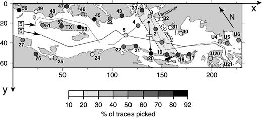
Map of the Strait of Georgia showing the region covered by the 3-D velocity model. Numbered dots are receiver station locations. Stations 1–5 are OBSs. Stations starting with a ‘U’ are located in the US. Grey-scale coding of dots, based on the percentage of traces recorded at the station that could be picked for first arrivals, gives an indication of data quality for each station. Dotted lines within waterways are shot point locations along the ship track. Numbers within squares identify the two seismic lines used in this study. The shaded rectangular region indicates the five receiver sites used in the 2-D study. Shots along line 5 between stations 19 and OBS 3 were used in the 2-D study. The heavy, short line segment just south of station 19 marks the location of a near-vertical boundary inferred from the 2-D modelling, assuming that the structure originates from within the line of shots and receivers. The solid line connecting two black diamonds just west of the 2-D line marks the location of a sonobuoy (diamonds) survey (White & Clowes 1984). The white rectangle in the middle of the sonobuoy line marks the location of a fault inferred by White & Clowes (1984). TXI, Texada Island.
The onshore–offshore shot–receiver recording geometry provides a set of ray paths that are not ideal for constraining the 3-D velocity structure. For example, except in the case of the OBSs, there are no shot points in the vicinity of the receivers. Thus, the near-surface velocity structure will not be well-constrained due to a lack of relatively short-offset ray paths. In addition, the narrow (230.4 km × 64.8 km) study region necessarily results in anisotropic 3-D ray coverage. All of the long-offset, deeper-penetrating ray paths will travel predominantly along the strait (x-direction). Ray paths crossing the strait will be limited to offsets of < 60 km and will therefore penetrate only the uppermost crust (3–4 km). The limitations of both the ray coverage and the recording geometry will be quantitatively assessed using a resolution test to be presented later.
Data quality is generally good; however, the signal-to-noise ratio (SNR) is correlated with the local site conditions. For example, sites 30–32 (Fig. 2) are located on thick sediments relatively close to large urban areas and have a very poor SNR. In contrast, site 50 is located on bedrock in a remote area and has an excellent SNR (Fig. 3a). The dominant frequency of the data is 6–8 Hz, implying a wavelength of 0.4–1.1 km for P-wave velocities of 3–6.7 km s−1. First arrivals at all offsets for all but the OBS stations are refractions through the upper crust with typical apparent velocities of ≈ 6.2–6.5 km s−1. At some sites (e.g. site 17; Fig. 3b), there is clear evidence for a thick layer of slower velocity (5.5 km s−1) material. Although first arrivals are visible up to maximum offsets of 200 km, the number of first arrivals at offsets greater than the expected crossover distance for upper mantle arrivals (≈ 180 km; Zelt . 1993) are few. Because of this, we confine our study to the crustal structure by restricting the maximum offsets in our analysis to 180 km.
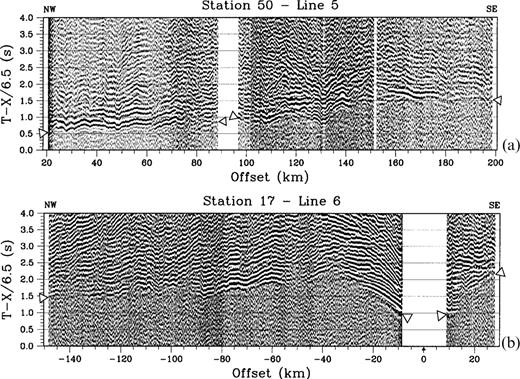
Record sections for (a) shots from seismic line 5 recorded at station 50; and (b) shots from seismic line 6 recorded at station 17 (Fig. 2). In both sections, data have been bandpass filtered between 4 and 10 Hz and reduced at 6.5 km s−1. Every third trace is plotted in both sections. Triangles mark locations of first arrivals.
A total of ≈ 115 000 first-arrival traveltime picks were obtained from the data set. For the 3-D tomographic inversion, the data were decimated to 20 547 picks by setting the minimum allowed distance between accepted shots to 350 m; tests showed that there were no significant differences in the final models obtained using the entire data set and the decimated data set. Pick uncertainties between 35 and 150 ms were estimated using an automated scheme based on an empirical relationship between uncertainty and SNR in short (250 ms) time windows on either side of the pick (Zelt & Forsyth 1994). The average estimated uncertainty of the data is 90 ms.
The 2-D study uses shots from seismic line 5 between stations 19 and OBS 3 recorded at five stations (19, OBSs 1–3, and 33; Fig. 2). These shots and receivers delineate a north–south crossing of the Strait of Georgia at about x = 150 km in the 3-D model. A total of six distinct phases were used in the modelling: Ps, Pg1, Pg2 and Pg3 are refractions which turn through increasingly deeper model layers; Pr are reflections from a near-vertical boundary near the south edge of the model; Sg3 are S waves converted at the water–sediment interface with ray paths similar to Pg3. Table 1 lists the phases used in the 2-D analysis and the associated average uncertainties.
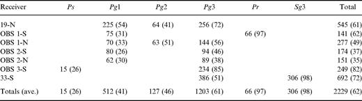
Number of picks (average uncertainty in ms) for phases used in the 2-D analysis ‘-N’ and ‘S’ after the station name refer to data recorded to the north or south, respectively, from the station. Ps are refractions through shallow sediments; Pg1 are refractionst hrough layers 4 and 5; Pg2 are refractions through layer 6; Pg3 are head waves along the top of layers 8 and refractions through layer 8; Pr are reflections from a near-vertical boundary near the south edge of the model; Sg3 are S waves, converted at the water—sediment interface, travelling as head waves along the top of layer 8 and refracting 8. Fig. 6(a) shows the numbered layers.
4 Method And Modelling Procedure
4.1 3-D modelling
The 3-D velocity structure is determined using first-arrival traveltime tomography. We use the regularized inversion algorithm described in Zelt & Barton (1998), with modifications to minimize the size and roughness (i.e. first or second spatial derivative) of the perturbation from a background model. This algorithm is flexible and is well suited for problems in which the ray coverage is sparse and/or anisotropic, because it allows for variable weighting with depth of any combination of smallest, flattest and smoothest perturbation constraints. In addition, the amount of regularization is determined automatically to ensure that a normalized χ2 data misfit of 1, if possible, is achieved. To account for non-linearity, the method is iterative and thus requires a starting model; new ray paths are calculated for each iteration. For the forward step, traveltimes are calculated on a uniform 3-D grid using a finite difference solution to the eikonal equation (Vidale 1990), with modifications to handle large velocity gradients and contrasts (Hole & Zelt 1995).
The velocity model dimensions are 230.4 km × 64.8 km × 18.4 km (Fig. 2), with the top of the model at 1.2 km above sea level. All depths mentioned in this paper are relative to sea level (0 km model depth). The forward modelling was performed on a uniform grid with a node spacing of 0.8 km; a cell size of 2.4 km × 2.4 km × 0.8 km was used for the slowness grid in the inverse step.
Several tomographic tests were performed to determine the optimal choice of free parameters controlling the type of regularization, the variation of the regularization with depth, and the relative importance of maintaining vertical versus horizontal roughness. For our preferred final model, we use only smoothing regularization and do not vary the weighting of the regularization with depth. Following the notation of Zelt & Barton (1998), we set sz = 0.225; this factor, which can be any value ≥ 0, controls the relative weighting of the vertical versus horizontal smoothing regularization, with a value of 0 resulting in no constraints on vertical smoothness. We found that this approach gave us the smoothest model overall, which provides a fit to the data of χ2 = 1.
The average first-arrival traveltime versus offset for the entire data set, calculated in 2-km-wide bins (Fig. 4a), was used to derive a simple 1-D (laterally homogeneous) starting velocity model by trial and error forward modelling. To eliminate ray focusing effects caused by discontinuities, the resulting 1-D model was smoothed slightly to produce the preferred 1-D starting model (Fig. 4b). The first-arrival times versus offset (Fig. 4a) are best fit by a nearly straight line with an apparent velocity of ≈ 6.2 km s−1 for offsets > 20 km, suggesting, on average, that the vertical velocity gradients in the crust are low. Because of the low average vertical gradients, ray coverage is limited to a maximum depth of about 13 km.
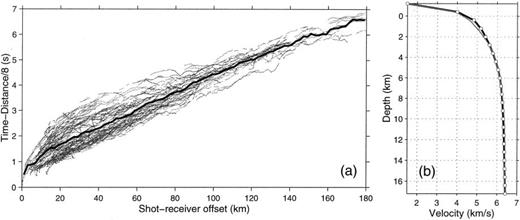
(a) Arrival times (reduced at 8 km s−1) for the 20 547 picks (dots) used in the 3-D modelling plotted against shot–receiver offset without regard to position or azimuth. Solid black line represents the average time in 2-km-wide offset bins used to construct the starting 1-D velocity model. (b) Black line is the smoothed 1-D starting model derived from the solid black line in (a). Dots indicate the starting velocity, at each depth level, of the finite difference model. The grey line is the average 1-D velocity structure of the final 3-D model.
Fig. 5(a) shows the traveltime residuals as a function of offset for the starting model. The initial normalized χ2 misfit was 44.6; the starting RMS traveltime residual was 470 ms. The final model was obtained after seven iterations with χ2 = 1 and an RMS traveltime residual of 72 ms; the final traveltime residuals are shown in Fig. 5(b). The bias near 0 km offset in the final residuals indicates that the near-receiver data at the five OBSs are misfit because velocity variations in the near-surface sediments could not be accurately represented or recovered using a vertical cell dimension of 0.8 km; nevertheless, the average near-surface cell velocity is considered representative of the true average.
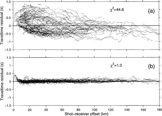
Traveltime residuals for (a) the 1-D starting model, and (b) the final 3-D model plotted against shot–receiver offset. The bias near 0 km offset in (b) results from poor fitting of the near-receiver data at the five OBSs.
4.2 2-D modelling
To derive the 2-D velocity structure along a profile between stations 19 and 33, we used the damped least-squares traveltime inversion algorithm of Zelt & Smith (1992). The 2-D model was derived prior to, and thus not biased by, the 3-D model (Zelt & Ellis 1999). In contrast to the 3-D tomography procedure, which uses a fine-grid parametrization and yields a minimum-structure model, the Zelt & Smith algorithm yields a blocky, ‘minimum-parameter’ style of model. Boundary nodes define layer boundaries; linear interpolation between upper and lower velocity nodes, tied to the upper and lower boundaries of a layer, defines the velocity structure within each layer. Any arbitrary combination of boundary and velocity nodes can be solved for by inverting the arrival times of various phases.
Fig. 6(a) shows the structure of the final 2-D velocity model, including the location of boundary and velocity nodes solved for by inversion. We employed a layer-stripping procedure in which progressively deeper structure was modelled whilst the more shallow structure was kept fixed. Vertical velocity gradients were fixed during inversions. Not all boundary and depth nodes were determined by inversion because the traveltime data were unable to constrain adequately all regions of the model. The base of the uppermost (water) layer was determined from bathymetry data. Velocities in layer 2 were set to 1.6 km s−1 following the example of White & Clowes (1984). The Pr phase was forward modelled to constrain the position of a short, near-vertical ‘floating’ reflector (Zelt & Forsyth 1994). The Sg3 phase was forward modelled by adjusting the average Poisson's ratio of the model beneath the water layer. All data (2229 arrivals) were fit to within their estimated uncertainties (normalized χ2 value of 1).
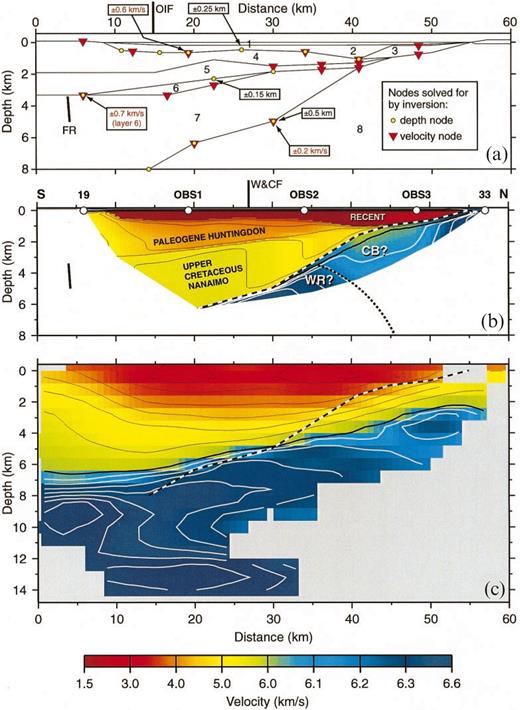
(a) Structure of the 2-D velocity model for a north–south profile between stations 33 and 19 (Fig. 2) showing boundaries (black lines), numbered layers, and depth (circles) and velocity (triangles) nodes solved for by inversion. Near-vertical thick black line at the left within layer 7 is a ‘floating’ reflector (FR) discussed in the text. Numbers within boxes are estimated absolute uncertainties of selected depth and velocity nodes. OIF marks the surface location of the Outer Islands fault. (b) Colour display of velocity for the 2-D model with simple geological interpretation. The white region is unconstrained. Circles at the top show receiver locations along the 2-D line. The heavy black and white dashed line is the boundary between basin sediments and underlying basement rocks (top of layer 8). The heavy black line is the 6 km s−1 isovelocity contour. The contour interval for velocities < 6 km s−1 is 0.5 km s−1 (thin black lines); for velocities > 6 km s−1, the contour interval is 0.1 km s−1 (white lines). The north-dipping dotted line depicts the speculative location of the boundary between the Wrangellia and Coast Belt rocks described in the text. W & CF marks the surface location of a fault inferred by White & Clowes (1984). WR?, Wrangellia?; CB?, Coast Belt? (c) A slice through the 3-D velocity model at the location of the 2-D profile. The heavy black and white dashed line and contour intervals are identical to those in the 2-D model. The colour scale at the bottom applies to (b) and (c). Vertical exaggeration is 2:1 in all panels.
5 results
5.1 3-D tomography results and resolution analysis
Horizontal slices through the final model at depths between 1 and 12 km are shown in Fig. 7. The dominant feature is the relatively low velocities at the southeastern end of the model at depths of less than 10 km. In vertical cross-sections orientated along the strait (Fig. 8a–c), this feature is recognized as the wedge-shaped region of relatively low velocities, increasing in thickness to the southeast. We interpret the low velocities (< 6 km s−1) as sediments of the Georgia Basin; however, because we do not know the velocity at the base of the sediments and because it may vary throughout the study area, this choice of isovelocity contour is somewhat arbitrary. We defer further discussion of the velocity model until after we have examined the resolution and constraints provided by the wide-angle data.
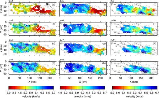
(a)–(l) Horizontal slices through the final velocity model at depths of 1–12 km. White dots are receiver locations. Regions not sampled by ray paths are shown in white. Velocity contour (black and white lines) interval is 0.2 km s−1 in all panels. The thick black contour is 6 km s−1. Note that colour scales are not linear and different scales are used for panels (a)–(d), (e)–(h) and (i)–(l). The star in (c) denotes the approximate hypocentral locations of the 1975 and 1997 earthquakes discussed in the text.
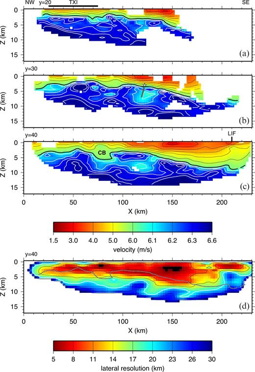
(a)–(c) Vertical slices through the final velocity model along the x-axis at y = 20, 30 and 40 km. The thick black line is the 6.0 km s−1 contour. The contour interval is 0.5 km s−1 for velocities < 6 km s−1 (black lines) and 0.1 km s−1 for velocities > 6 km s−1 (white lines). Regions not sampled by ray paths are shown in white. Note that the colour velocity scale is not linear. The star in the y = 30 km panel denotes the approximate hypocentral location of the 1975 and 1997 earthquakes discussed in the text. The yellow line below the star depicts the dip of the fault plane (Cassidy . 2000). The black line labelled TXI above (a) marks the location of Texada Island. In (c), LIF is the surface location of the Lummi Island fault; CB marks a possible local increase in thickness of the Comox sub-basin. (d) Estimated lateral resolution along the y = 40 vertical slice; the contour interval is 5 km. The white contour is 20 km. The dotted line is the 6 km s−1 contour, taken to represent the base of the basin, from (c). Black regions have a better than 5 km resolution; white regions have a worse than 30 km resolution or are unsampled. Vertical exaggeration is 3:1.
Regions of the model constrained by data are indicated in plots of the number of rays penetrating each cell of the velocity model (Fig. 9). Ray coverage peaks at 3–5 km depth because of the relatively large number of short-offset rays travelling in all directions. Below this there are large regions in the interior of the model with poor ray coverage. At depths > 9 km there are no rays with bottoming points northwest of x = 50 km. Southeast of this, however, there are significant regions with good ray coverage (> 20 rays per cell). The long-offset, deep-penetrating ray paths travel predominantly along the Strait of Georgia in the x-direction, giving rise to significant anisotropy in the deep ray coverage.
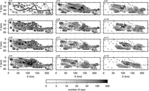
Horizontal slices of ray coverage measured as the number of rays penetrating each cell of the final model at depths between 1 and 12 km. Coastline and shot locations are shown in the z = 1 km panel. White dots in all panels are the receiver locations. Contours are drawn at 1, 5, 10, 25, 50, 100 and 250 km. The thick black line is the 25 km contour. For clarity, contours are omitted in the z = 1 panel. Regions not sampled by ray paths are white.
Although plots of ray hit counts provide useful visual information regarding the location and density of data constraints, they do not quantitatively indicate the ability of the data to resolve model features of a particular length scale. In order to assess quantitatively the resolution of the data, we perform checkerboard resolution tests and use the results of these tests to generate maps of estimated lateral resolution at each point of the model using the method described in Zelt (1998).
For the checkerboard tests, we added a checkerboard anomaly pattern to the preferred final model and generated synthetic data for the same distribution of shots and receivers as used in the actual experiment. Gaussian noise, with a standard deviation equal to the pick uncertainties, was added to the synthetic data. Using the preferred final model as a starting model, we tried to recover the perturbed model using the same procedure and the same free parameter values as used for modelling the real data. Regions of the recovered model perturbation that resemble the checkerboard pattern are considered to be well resolved at the length scale of the checkerboard anomaly. The checkerboard anomaly pattern comprises a grid of squares with alternating ± 10 per cent velocity perturbations from the final model, varying only in the horizontal direction. The 10 per cent variation from the final model is large enough to provide a traveltime perturbation above the noise level of the data, without significantly perturbing the ray paths in comparison to the final model, and thus not invalidating the linearization assumption of the tomographic approach. We used four anomaly sizes: 5, 10, 20 and 30 km; for each anomaly size we used eight different anomaly patterns that varied in their orientation, registration and anomaly polarity (Zelt 1998). Exemplary recovered anomaly patterns for the 10, 20 and 30 km anomaly sizes, shown in Fig. 10, illustrate the vertical and lateral variations in resolution. At 2 km depth, the 10 km checkerboard pattern is well recovered in regions constrained by the data. At 8 km depth, the three lower right cells of the 30 km checkerboard are reasonably well recovered, suggesting a lateral resolution on the order of 30 km here, but greater than 30 km elsewhere.
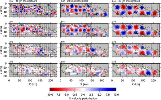
Representative results of checkerboard tests using checkerboard cell sizes of 10 km (left panels), 20 km (centre panels) and 30 km (right panels). Horizontal slices of relative velocity perturbations with respect to the starting model are shown for depths of 2, 4, 6 and 8 km for each checkerboard cell size. Boundaries of the true checkerboard pattern are indicated by grid lines. The true checkerboard pattern is a ± 10 per cent velocity variation from the final model. Regions not sampled by ray paths in the final model are shown in grey. Dots are receiver locations.
To estimate the lateral resolution at each point of the velocity model, we follow the method described by Zelt (1998). For each anomaly size the semblance between the recovered anomaly and the true anomaly at each point, calculated using a semblance operator with a radius of 10 km, is averaged for the eight different patterns. The averaged semblance is called ‘resolvability’ by Zelt (1998); nodes with resolvability values greater than 0.7 are considered ‘well resolved’. The lateral resolution at each node is then determined by interpolating to obtain the anomaly cell size that gives a resolvability value of 0.7. The average lateral resolution as a function of depth increases approximately linearly from about 10 km at 2 km depth to 30 km at 12 km depth (Fig. 11). At depths of z ≤ 4 km, the lateral resolution is better than 20 km within the region bounded by the receivers, and better than 10 km for more than half of this part of the model. The good shallow resolution reflects the more isotropic ray coverage here. Below 9 km depth the resolution is worse than 20 km throughout most of the model. As the depth increases the best resolution is obtained near the southeastern end of the model, where there is more deep ray coverage because of the effect of the relatively high vertical velocity gradient in the basin. Fig. 8(d) shows lateral resolution for a vertical slice at y = 40 km. In general, and as seen in this slice, resolution is better than 20 km to depths of 3–5 km below the base of the basin.
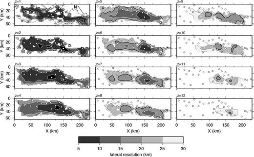
Horizontal slices of estimated lateral velocity resolution at depths between 1 and 12 km using the method of Zelt (1998). The contour interval is 5 km. The heavy black line is the 20 km contour. Contours for lateral resolution < 20 km are white. For clarity, contours are omitted in the z = 1 panel. Black regions have a better than 5 km resolution; white regions have a worse than 30 km resolution or are unsampled. Dots are receiver locations.
5.2 2-D inversion results and uncertainties
The layered structure of the model and boundary and velocity nodes solved for by inversion are shown in Fig. 6(a). Velocities within the final model are shown in Fig. 6(b). Ray diagrams, indicating the degree to which various parts of the model are sampled for each station, and a comparison of observed and calculated traveltimes for each station, are shown in Fig. 12. The velocity model comprises eight layers, some of which are included to allow changes in the vertical velocity gradient. Velocities are constrained to a maximum depth of 6 km. The absolute uncertainties of a number of parameters determined by inversion were estimated using the method described by Zelt & Smith (1992). This method involves perturbing and fixing a parameter whilst inverting the other parameters that were determined simultaneously with the perturbed parameter when deriving the final model. The maximum perturbation for which the recovered model fits the observed data is an estimate of the parameter's absolute uncertainty. The estimated uncertainties are quite variable: errors in the three depth nodes tested range between ± 0.15 and ± 0.5 km; errors in the three velocity nodes tested range between ± 0.2 and ± 0.7 km s−1 (Fig. 6a).
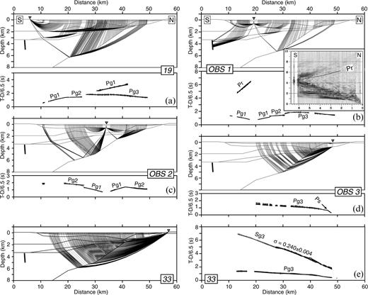
(a)–(e) Ray diagrams and comparisons between observed (short vertical lines corresponding to pick uncertainties) and calculated (dots) traveltimes for the five receivers used in the 2-D analysis. The dots are close enough together that they frequently appear as a line. The dashed-line ray paths in (e) represent S waves. See Table 1 for a description of the phases. Inset in (b) shows the Pr phase recorded on the near-offset traces at OBS 1; the y-axis is the time reduced at 6.5 km s−1; the x-axis is the distance from the receiver.
The velocity model can be divided into four distinct regions (excluding the water layer) on the basis of velocity. Layers 2 and 3 extend to a maximum depth of 1 km with velocities of 1.6–2.5 km s−1. There was no direct velocity control for layer 2 and thus velocities were fixed at 1.6 km s−1 (White & Clowes 1984). Velocities in layer 3, which exists north of the 40 km model distance, were constrained by a short phase recorded at OBS 3 (Ps in Fig. 12d). Velocities in layers 4 and 5 are 3.8–5.0 km s−1. Velocities in layers 6 and 7 are generally 5.0–5.5 km s−1. Velocities in the region sampled by rays in layer 8 are 6.0–6.5 km s−1, with the lowest velocities occurring in the region between 40 and 50 km model distance. The dip on the boundary at the top of layer 8, south of 40 km, is approximately 12° to the south. An interesting, but clear, late phase (Pr) recorded on OBS 1 (Fig. 12b, inset) was modelled as a reflection from a short, near-vertical ‘floating’ reflector located just south of station 19, at a depth of 4–5 km. This location, of course, assumes that the reflector is located in the plane of our model, but it is possible that the Pr phase may be associated with a structure located significantly out of this plane. In addition, the location of the reflector is only approximate because the Pr ray paths travel in part through a region of the model where there are no direct constraints on the velocity (Fig. 6). The lack of a Pr phase at the other stations, however, is consistent with its location as modelled because observable reflections from this boundary to stations other than OBS 1 are not possible.
6 Discussion
6.1 3-D velocity model
The tomographic velocity model (Figs 7 and 8) clearly delineates the relatively low-velocity sedimentary rocks of the Georgia Basin. These primarily comprise conglomerate, sandstone, siltstone and shale of the Upper Cretaceous Nanaimo Group and overlying Huntingdon Formation, as well as Pleistocene glacial deposits and modern Fraser delta sediments. Taking the 6 km s−1 isovelocity contour to represent seismic basement suggests that the Georgia Basin is approximately 2–4 km thick northwest of x = 125 km; southeast of this the basin increases in thickness with a dip of ≈ 5° to approximately 9 km at x = 175 km (Fig. 13). These values are consistent with results from preliminary gravity modelling (Lowe & Dehler 2000) and a preliminary interpretation of SHIPS seismic reflection data from the southern half of shot line 6 (Mosher . 2000). The maximum depth of the basin (8–9 km) occurs near the southeastern end of our region of constraint, which is close to the southeastern edge of the Georgia Basin. It is unlikely that the basin achieves a greater depth further to the southeast; however, if the basin is fault-bounded at the southeast end in a manner analogous to the southern bounding of the Seattle basin by the Seattle fault (Pratt . 1997; Johnson . 1999), this boundary is outside our region of constraint. Regardless, in terms of maximum sediment thickness, at 8–9 km, the Georgia Basin appears to be equivalent to other basins to the south, such as the Seattle Basin (Brocher . 1999a; Crosson . 1999; Molzer . 1999). It is interesting to note the increase in depth of the 6 km s−1 isovelocity contour at x = 205 km along the y = 40 km slice (Fig. 8c). This is a position which corresponds very closely to the Lummi Island fault (Fig. 1), which separates the Whatcom and Chuckanut depocentres, and across which there is believed to be at least a 1.5 km drop down to the south (Miller & Misch 1963; Johnson 1985). However, given the poor lateral resolution in this region of the model (> 20 km) (Fig. 8d), the correlation may not be significant.
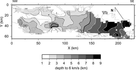
Contour map of depth to the 6 km s−1 isovelocity contour in the final 3-D velocity model, which is interpreted to represent approximately the base of the Georgia Basin sediments. The contour interval is 1 km. The heavy black line is the 5 km contour. Contours for depths > 5 km are white. Co, Na and Wh are the Comox, Nanaimo and Whatcom sub-basins, respectively.
Northwest of x = 100 km, basin velocities are typically ≥ 4.5 km s−1; southeast of this, velocities in the upper 3 km are noticeably slower (3–5 km s−1; Figs 8a–c). The relatively slower shallow velocities in the southeast reflect the presence of significant accumulations of the Tertiary Huntingdon Formation (Chuckanut Formation at the extreme southeastern end of the model) and overlying younger sedimentary deposits. There is evidence for a local increase in the thickness of the Comox sub-basin on the southwest side of the Strait of Georgia at x = 80 km, where the 6 km s−1 isovelocity contour is depressed to 6 km depth (Figs 8c and 13). Of course, if the velocities at the base of the sediments are < 6 km s−1, this depression would represent a region of relatively low-velocity basement rocks.
Isovelocity contours above the 6 km s−1 contour are moderately flat, revealing a simple increase in velocity with depth (Figs 8a–c). In contrast, isovelocity contours below this line reveal significantly more structure, with maximum velocities of about 6.5 km s−1. Of course, structures with dimensions less than the estimated lateral resolution (Figs 11 and 8d) are probably not significant, and are possibly caused by anisotropy in the ray coverage, or an effect of the poorer ray coverage at depth. It is clear, however, that there is significant velocity variation even at large, well-resolved scales. For example, velocities are relatively high directly beneath the basin in the vicinity of Texada Island (x = 50 km), and further south at about x = 150 km (Figs 8b and c). Although lower in amplitude, a third region of relatively high sub-basin velocities occurs about halfway between these two zones. These variations in basement velocity probably represent velocity variations between the various lithologic units comprising Wrangellia, for example, basaltic lavas of the Upper Triassic Karmutsen Formation, sediments and intermediate volcanics of the mid-Palaeozoic Sicker Group, and Mesozoic intrusive rocks.
Hypocentres for the 1975 (M = 5) and 1997 (M = 4.6) Georgia Strait earthquakes (stars in Figs 1 and 8b) and aftershocks define a northward-dipping plane with a dip angle of 53° between depths of 2 and 4 km (dipping line on Fig. 8b; Cassidy . 2000). Lateral resolution in the vicinity of the hypocentres is good (5–10 km), suggesting a possible correlation between the fault plane position and relatively low sub-basin velocities below the hypocentres (6.1–6.2 km s−1). Farther to the southwest, the y = 40 km slice (Fig. 8c) also reveals a decrease in velocity at roughly the same lateral position (x = 130 km), separating two high-velocity anomalies immediately below the basin. If the correlation between the fault plane as defined by the hypocentres and the low-velocity regions is meaningful, then the actual fault plane may be significantly larger in extent than suggested by the distribution of hypocentres.
6.2 2-D velocity model
A complementary view of the Strait of Georgia structure is provided by the 2-D interpretation of the north–south profile between stations 19 and 33 (Fig. 6b). The 2-D interpretation method allowed for a more detailed, although more subjective, analysis of this small subset of the data. Whilst both the 2-D and 3-D models provide overall normalized χ2 misfits of 1.0 to their respective data, the misfit for the 3-D model calculated using only data from shots and receivers used in the 2-D analysis is significantly higher (5.2) due to poor fitting of the near-offset data. Thus, in a strictly 2-D sense, the 2-D velocity model in Fig. 6(b) can be considered better focused than the corresponding slice through the 3-D model (Fig. 6c). The 3-D model, however, is additionally constrained by out-of-plane data. A comparison of the 2-D model with the slice through the 3-D model shows a general agreement in the overall velocity structure. In both models, the 6 km s−1 isovelocity contour, which we take as the base of the basin, dips southward, with the boundary in the 2-D model dipping more steeply. Basin velocities are similar; however, the three distinct velocity layers in the 2-D model (Fig. 6b) are not resolved in the 3-D model (Fig. 6c) because of the smoothing inherent in the minimum-structure inversion procedure. The uppermost basin velocities, to a depth of ≈ 1 km in the 2-D model, which probably represent modern unconsolidated Fraser River sediments and Pleistocene glacial deposits, are lower (1.6–2.5 km s−1) but, with the exception of near OBS 3, the velocities here are not directly constrained by the seismic data.
The second layer in our interpretation (layers 4 and 5 of the velocity model; Fig. 6a), with velocities of 3.8–5.0 km s−1, represents sediments of the Tertiary Huntingdon Formation and possibly the Neogene Boundary Bay Formation, whilst the third layer (layers 6 and 7 of the velocity model), with velocities of 5.0–5.5 km s−1, represents sedimentary rocks of the Upper Cretaceous Nanaimo Group.
Sub-basin velocities, where constrained in the 2-D model, are 6.0–6.4 km s−1. The basement comprises Palaeozoic to Jurassic rocks of the Wrangellia Terrane and/or Jurassic to mid-Cretaceous granites and granodiorites of the Coast Belt. The variable velocities here may be a signature of the transition zone from Wrangellia to Coast Belt rocks. In this interpretation, the depressed isovelocity contours between 40 and 50 km model distance (Fig. 6b) would represent Coast Belt rocks (CB); the higher velocities to the south represent Wrangellia (WR), whilst the higher velocities to the north may indicate the presence of a slice of Wrangellia, which is known to crop out in the western Coast Belt (Journeay & Friedman 1993). From potential field data, Clowes . (1997) interpreted a northeast-dipping contact between Wrangellia and Coast Belt rocks beneath the Strait of Georgia, with the shape of the boundary varying along strike. The north-dipping dotted line separating Wrangellia from Coast Belt rocks in Fig. 6(b) is consistent with their interpretation, if somewhat speculative given the constraints provided by our data. The corresponding slice through the 3-D model (Fig. 6c) contains similar evidence for a reduction in velocity between 40 and 50 km model distance. This is not, however, a laterally continuous feature along the x-axis of the 3-D model. On the other hand, such a feature, if present, would generally not be well resolved by our 3-D data because of the poor ray coverage at sub-basin depths along the northeastern (y < 20 km) edge of our model.
In a shallow (< 3 km) sonobuoy study within the Strait of Georgia, White & Clowes (1984) proposed the existence of a near-vertical fault with a throw of 0.55 km on a line ≈ 10 km west of our 2-D line (Fig. 2). The fault, which projects to the surface between our OBS 1 and OBS 2, is not consistent with our data; such a fault would generate a distinctive offset in the first arrivals of ≈ 0.35 s. This suggests that the fault is either localized to their nearby line, or that the data of White & Clowes (1984) were misinterpreted due to sonobuoy drift, non-coincidence of their reversed profiles, and relatively sparse data.
The short, north-dipping, near-vertical boundary below station 19, modelled as a ‘floating’ reflector (Fig. 6b), bears a remarkable resemblance to a steep, northeast-dipping extensional fault interpreted on an old (1970) and short reflection profile located approximately 10 km east of our 2-D line and between station 19 and OBS 1 (England & Bustin 1998). The fault, referred to as the Outer Islands fault (Figs 1 and 6a), appears to offset the Tertiary and Cretaceous sedimentary layers on the southwestern side of the Strait of Georgia (England & Bustin 1998). The inferred location of the Outer Islands fault (Fig. 1) is inconsistent with the location of the boundary imaged by our 2-D data; however, given the possibility that both interpretations may be based on out-of plane structures, it is possible that both data sets are imaging the same boundary. Perhaps more plausibly, the boundary in our 2-D model may be a steep thrust fault associated with the northwest-trending mid-Eocene Cowichan fold-and-thrust system, comparable to the fault labelled ‘A’ in Fig. 1.
A clear S-wave phase recorded at station 33 gives an average Poisson's ratio of 0.240 ± 0.004 for ray paths shown in Fig. 12(e). In comparison, Mulder & Rogers (1998), using the difference between P and S arrival times of local earthquakes, estimated Poisson's ratio values of 0.259 ± 0.002 for the upper crust of Wrangellia on Vancouver Island, and 0.240 ± 0.002 for the upper crust of the Coast Belt. On this basis, they concluded that the suture zone between the Wrangellia and granitic rocks of the Coast Belt lies beneath the Strait of Georgia, as suggested above based on our results, or at the very western edge of the Coast Belt. Our Poisson's ratio value suggests that, on average, the region sampled by ray paths bears a closer affinity to Coast Belt composition. A meaningful comparison between results, however, is difficult; based on the interpretation shown in Fig. 6(b), the S-wave ray paths are probably travelling through both Wrangellian and Coast Belt basement rocks, in addition to Nanaimo sediments, which have a high quartz content and thus presumably a low Poisson's ratio, and younger sediments with possibly relatively high Poisson's ratios.
7 Conclusions
By a tomographic inversion of first-arrival traveltimes we have derived a minimum-structure 3-D velocity model for the upper 13 km of the crust beneath the Strait of Georgia. Using the 6 km s−1 isovelocity contour as a proxy for the top of the basement, we are able to map the thickness variations of the Cretaceous to Cenozoic Georgia Basin throughout the Strait of Georgia (Fig. 13). The basin is 2–4 km thick in the northern part of the strait. Southeast of Vancouver, the basin increases to a maximum thickness of about 9 km at the southeastern end of the strait. These variations are consistent with variations in the Bouguer gravity anomaly (Lowe & Dehler 2000) and a preliminary interpretation of SHIPS reflection data (Mosher . 2000). The thicker sediments in the southeast reflect the presence of significant accumulations of the Tertiary Huntingdon Formation and younger deposits overlying the Upper Cretaceous Nanaimo Group. Lateral variations in sub-basin velocities indicate far more structure, associated with lithologic variations in the basement rocks, in comparison to the overlying sediments. The 2-D velocity model for a north–south-orientated profile located just west of Vancouver more clearly differentiates the velocity layering associated with the sediments and underlying basement rocks.
The 3-D velocity model does not directly image the fault plane associated with the 1975 and 1997 Strait of Georgia earthquakes; however, a vertical cross-section along the x-axis at the location of the hypocentres does reveal a relative decrease in velocity in this region. An interesting reflected phase recorded at OBS 1 (Pr;Fig. 12b) was modelled as a reflection from a near-vertical boundary, perhaps associated with the Cowichan fold-and-thrust belt (Fig. 1), just south of station 19.
Lateral resolution in the 3-D velocity model decreases with depth but is typically better than 20 km to depths of 3–5 km below the top of the basement. The narrow onshore–offshore recording geometry is not ideal for 3-D tomography because of the anisotropy of the ray coverage. Because this limitation can give rise to artefacts in the velocity model, the use of a regularized inversion technique, which minimizes the roughness of the slowness perturbation from a background model (e.g. Zelt & Barton 1998), is important because it seeks a model with only those features required by the data, as opposed to merely being consistent with the data.
Acknowledgments
We thank the numerous individuals who participated in the fieldwork. Special thanks to Keith Louden of Dalhousie University for supplying the ocean bottom seismometers, and retrieving and converting the data to SEGY format. Other people who were instrumental in making the SHIPS program successful were Tom Brocher and Tom Parsons in the US, and Dave Mosher and Phil (the human logician) Hammer in Canada. We gratefully acknowledge a constructive review of an earlier version of this manuscript by Ron Clowes. We also thank Tim Henstock and Tom Brocher for their reviews and many helpful suggestions.
Funding for SHIPS was primarily through the USGS National Earthquake Hazards Reduction Program (NEHERP). The Canadian component, including the use of two ships, was additionally funded by the GSC. Land instrumentation was provided by the IRIS-PASSCAL consortium. Analysis of the data was funded by a Natural Sciences and Engineering Research Council of Canada research grant (RGPIN 2617). Data from the US receivers were provided by the IRIS/PASSCAL Data Management Center.
References
