


Summary
We present a fast and accurate analytical method for computing differential seismograms with respect to structural model parameters. The method adopts the P–SV‐wave multimode summation formalism for laterally homogeneous layered media. The differential seismograms calculated analytically do not suffer from the numerical noise and instability affecting numerical calculations. The frequency range for application of the method spans from regional‐scale seismology to seismic engineering. Computationally, the proposed analytical method is equivalent to determining two‐mode spectra. In contrast to N+ 1 (or 2N) mode spectra for a typical ‘brute‐force’ numerical finite difference approach, the method reduces the computations to 2/(N+ 1) (if a one‐sided perturbation finite difference scheme is used), which corresponds to a 90 per cent saving for 20 (N=20) layers. The speed and accuracy of the technique make it extremely attractive for structural parameter waveform inversions.
1 Introduction
Aided by the large quantity of accumulated broad‐band waveform data, nowadays formal waveform inversion for medium structural parameters can be performed by adopting either global, non‐linear procedures such as the ‘hedgehog’ (Valyus 1972) and more recent variants represented by the genetic algorithm (Sambridge & Drijkoningen 1992) or simulated annealing (Sen & Stoffa 1991), or iterative, local linearization of the misfit function (e.g. Nolet 1990). In fact, these two classes of methods are not unrelated but are complementary, and through an appropriate combination they can often provide additional information about the structure of the Earth. The first class of methods requires extremely fast forward‐modelling procedures, whereas the second class, even if it needs many fewer forward calculations, still requires efficiency and accuracy for determination of the differential seismograms.
The first efforts to calculate differential seismograms for regional‐ and local‐scale waveform modelling were made by Shaw & Orcutt (1985) using the ‘WKBJ seismogram’ technique (Chapman 1978), and by Gomberg & Masters (1988), who proposed, within the locked‐mode approximation, a hybrid technique in which the differentiation of the phase term is performed analytically and that of the amplitude term numerically. More recently, methods based on the matrix formalism of Kennett (1983) and Luco & Apsel (1983) have been proposed by Randall (1989, 1994) and Zeng & Anderson (1995), respectively. In this paper, we present a technique to compute analytically complete differential seismograms for laterally homogeneous layered structures using the multimode summation formalism (Knopoff 1964; Schwab 1970; Schwab & Knopoff 1972; Panza 1985; Panza & Suhadolc 1987; Urban, Cichowicz & Vaccari 1993).
2 Method
Following Panza, Schwab & Knopoff (1973), for a given Rayleigh mode the displacement for an assigned point source double‐couple can be expressed in the frequency domain as
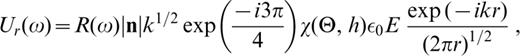
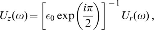
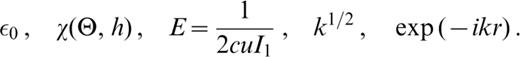
where R(ω) is the Fourier transform of the equivalent point‐force time function, χ is the source radiation pattern, n is the unit vector perpendicular to the fault surface and has units of length, k is the wavenumber, r is the epicentral distance, and ε0=uraise3*(0)/w(0) (uraise3*=calIm(u)) is the ellipticity calculated as the ratio of the radial and vertical components u(z) and w(z) of the Rayleigh‐mode eigenfunctions at the free surface.
The factor E is given by
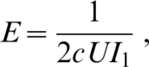
where c and U are the phase and group velocities, respectively. The energy integral is defined as
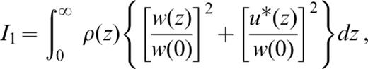
where ρ (z) is the density.
For a double‐couple point source (Harkrider 1970), χ (Θ, h), the source radiation pattern is

where


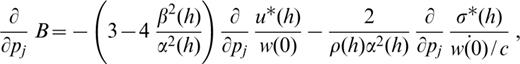
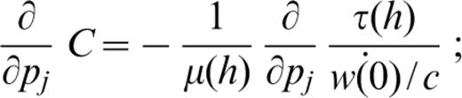
The source geometry is defined by the angles Θ, δ and λ, which are the azimuth of the station with respect to the fault strike, the fault dip and the slip angles, respectively. h is the source depth and A(h), B(h) and C(h) involve the eigenfunctions (i.e. the ‘motion–stress vector for Rayleigh waves’) at the source depth:
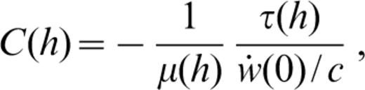
where an overdot indicates time differentiation and σ and τ are the normal and tangential stresses.
Eqs (1) and (2) are equivalent to expressions (7.149) and (7.150) of Aki & Richards (1980), who, however, express the source term through the seismic moment tensor.
3 Differential Seismograms
An efficient and accurate technique for computing differential seismograms with respect to structural parameters can be developed using eqs (1) and (2). In the following we restrict our formulation to a double‐couple point source, although the method can be easily extended to other types of seismic source (e.g. Das & Suhadolc 1996).
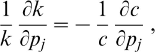
The terms of eqs (1) and (2), which depend on structural parameters, are
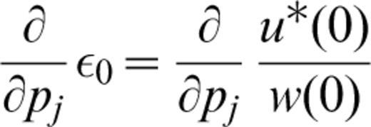
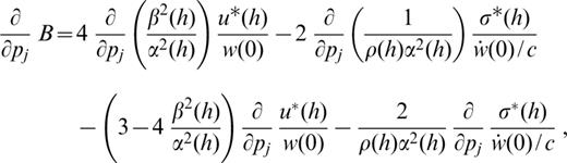
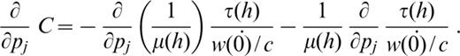
In detail, the partial derivative of ε0 with respect to structural parameters can be computed from the partial derivatives of the eigenfunctions with respect to the structural parameters (Appendix A). The partial derivative of χ (Θh) with respect to the structural parameters can be obtained from computation of the partial derivatives of A(h), B(h) and C(h) with respect to the structural parameters. For the discussion below, we define j as the layer sequential number and pj (i.e. α β and ρ) as the structural parameters. The partial derivatives are
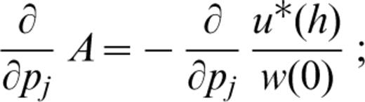
and
for the layers above and below the source,
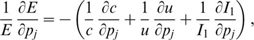
The computation of the partial derivatives for k and E with respect to the structural parameters involves the calculation of the partial derivatives of the phase and group velocities and of the energy integral with respect to the structural parameters:
where the partial derivative of phase velocity with respect to the structural parameters can be computed with the method described in Urban et al. (1993). By using (4), the partial derivative of the energy integral with respect to the structural parameters can be obtained from the partial derivatives of eigenfunctions with respect to the structural parameters (see Appendix A). Here the partial derivative of group velocity with respect to the structural parameters is computed with an asymptotic fast method, given in Appendix B.
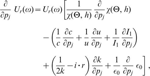
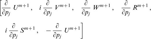
Once all the partial derivatives of the terms in (8) have been determined, the complete differential seismogram for a given P–SV mode can be constructed using the following expressions:
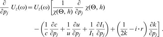
The radial component, (∂/∂pj)Ur, in (12) involves four terms, each being controlled by the physics of the problem. The first term, (1/χ (Θ, h))(∂/∂pj)χ (Θ, h), describes the source‐term changes caused by the model parameter perturbations. In fact, the seismogram source term is not local (Kennett 1995) in that the eigenfunction values at the source are affected by the perturbations in the structure. The second term accounts for the waveform changes resulting from perturbations in the medium properties. The first factor of the third term, (1/2k)(∂k/∂pj) results from the adoption of a point source in 3‐D space (see Chapter 7.4 of Aki & Richards 1980), whereas the factor −i˙r (∂k/∂pj) is the seismogram phase term change due to the structural perturbation. In the WKBJ‐type waveform inversion scheme (e.g. Nolet 1990), only this term is accounted for in the calculation of differential seismograms within the linearized inversion scheme. The last term, (1/ε0)(∂/∂pj)ε0, accounts for the deformation of elliptical particle motion induced by structural perturbation. The vertical component, (∂/∂pj)Uz, in (13) includes only the first three terms just described.
4 Analytic Versus Numerical Differentiation
In this section we compare the results of analytical calculations of differential seismograms with those obtained through ‘brute‐force’ numerical differentiation. The upper 250 km of the structure used to generate synthetic seismograms is shown in Fig. 1(a). While IASP91 velocity structure (Kennett & Engdahl 1991) is used at depths greater than 250 km, the density model in CAL8 (Bullen & Bolt 1985) is adopted for the same depths. From 250 to 640 km a constant Q of 450 is used, and a linear increase of Q of 450–680 is adopted to extend the structure down to a depth of 1060 km. Our structure has continental properties and it is characterized by two main velocity discontinuities. The source is located in the crust at a depth of 33 km and a double‐couple mechanism is adopted. The source parameters are δ=37°, λ=283°, and the azimuth of the station with respect to the fault strike is 260°, The seismograms have been scaled with a moment of 6.5 × 10¹⁹ N m, The top traces in Fig. 2 are the seismograms computed for a distance of 400 km from the source using an upper frequency limit of 1.0 Hz, whereas the top traces in Fig. 3 show the seismograms for an epicentral distance of 1000 km with an upper frequency limit of 0.1 Hz. A Gaussian roll‐off filter with corner frequencies of 0.85 and 0.085 Hz is used to remove the ringing arising from the truncation of the spectrum at frequencies of 1.0 and 0.1 Hz, respectively.
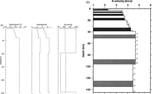
(a) Upper 250 km of the velocity model used to generate the seismogram synthetics and the differential seismograms; (b) enlarged upper part of the shear‐wave velocity model. The differential seismograms shown in Fig. 2 are computed with respect to shear‐wave velocity for the grey‐shaded layers. The whole structure used to determine the mode spectrum extends to a depth of 1060 km.
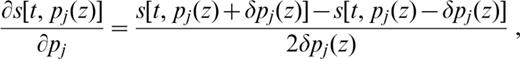
We compute the differential seismograms with respect to the change of shear velocity in each layer using a first‐order centred numerical differentiation. Each differential seismogram involves two seismogram evaluations, but guarantees some stability in the numerical differentiation. The adopted differentiation formula is
where δpj(z)=0.005 km s− 1 is the shear‐wave velocity perturbation. This evaluation is quite time‐consuming because the computation of s[t, pj(z)+δpj(z)] and s[t, pj(z)−δpj(z)] requires the determination of two additional modal spectra.
Our alternative approach for computing the differential seismogram is more direct and efficient than the numerical approach. As given by eqs (12) and (13), we take the partial derivative of the seismogram in the frequency/wavenumber domain, where analytical solutions exist, before carrying out the inverse transform to obtain the time‐domain differential seismogram. In practice, the computation time of this analytical calculation is approximately equal to one synthetic seismogram calculation.
In Figs 2 and 3 we show differential seismograms calcu‐lated analytically together with those determined numerically. For brevity, we show only the differential seismograms corresponding to the grey‐shaded layers of Fig. 1(b). For the 1 Hz upper frequency limit, we show the results obtained for one mantle layer (layer number 14) and five crustal layers (2, 4, 6, 8 and 12), since within this frequency range most wave energy is trapped in the crust. When the 0.1 Hz upper frequency limit is chosen, we show the results for three crustal layers (2, 8 and 12) and three mantle layers (14, 20 and 24). The solid lines correspond to the analytical calculations, whereas the dashed lines correspond to those obtained numerically.


Seismogram and differential seismograms computed with respect to shear‐wave velocity for the layers indicated in Fig. 1. The uppermost trace is the velocity seismogram (m s− 1), which is determined using an instantaneous point‐source double‐couple (δ=37°, λ=283° and h=33 km) located at a distance of 400 km and at a strike–receiver angle of 260°, The seismograms are scaled with a moment of M0=6.5 × 10¹⁹ N m. The remaining traces are the differential seismograms. The number at the top right of each seismogram indicates the layer number (Fig. 1b) to which the differentiation refers. A Gaussian roll‐off filter with a corner frequency of 0.85 Hz is applied to all traces to remove ringing due to truncation of the spectrum. (a) Radial component; (b) vertical component.


Same as Fig. 2, but with a source–receiver separation of 1000 km and a Gaussian roll‐off filter with a corner frequency of 0.085 Hz. (a) Radial component; (b) vertical component.
We see that the differences between the results using the two techniques are small. As expected, the analytical differential seismograms do not suffer from the numerical instabilities affecting the purely numerical differentiation (Figs 2 and 3). Computationally, as mentioned above, the numerical differentiation involves a total of 2N (N being the number of layers) or N+ 1 (if a one‐sided perturbation finite difference scheme is used) mode‐spectrum calculations. In contrast, the analytic method involves the calculation and storage of the relevant ∂ derivatives only once, and the total computational cost required is of the order of about one additional mode spectrum. It follows that the analytical method requires only fast access to the data file of the ∂ derivatives. If T is the time for a single mode‐spectrum computation, this results in a total time of 2T for the analytic method. In contrast, 2NT or (N+ 1)T is required for the conventional numerical technique. T is proportional to the number of layers, N, so the analytic method grows linearly with N, whereas the numerical technique grows quadratically with N. Depending on the number of layers, exact analytical differentiation leads to a consistent computational reduction, which for a 20‐layer model is as much as nearly two orders of magnitude or about 90 per cent reduction in CPU time compared with the conventional(one‐sided finite difference scheme) numerical approach. This represents a very large CPU time‐saving.
5 Discussion
A detailed discussion and complete analysis of the contributions provided by the different terms in eqs (12) and (13) is presented by Du & Panza (1998). Here we describe only the main features that characterize the differential seismograms shown in Figs 2 and 3.
In general, and besides their frequency dependence, the amplitudes of the differential seismograms depend on the layer thicknesses. In our structural model the thicknesses of the individual layers vary with depth, and these should be accounted for while comparing the effects on the differential seismograms of layer velocity change.
With an upper frequency of 1 Hz (Fig. 2) we observe that a comparable effect is obtained when the shallow and 2.0‐km‐thick layer 2 (between 2 and 4 km depth) and the 6‐km‐thick layer 12 (between 33 and 39 km depth) are perturbed. As expected, a perturbation of the shallow layer 2 gives a more pronounced effect on the tail of the seismogram. In contrast, a perturbation in the upper mantle (i.e. layer 14) affects only the early part of the synthetic seismogram (i.e. between 90 and 125 s). The shape of the differential seismograms in the crustal layers is quite stable and their amplitude changes are well marked by the major discontinuities in the structural model. Although the waveforms of the differential seismogram become simple, when a relatively low upper frequency limit of 0.1 Hz is used, as shown in Fig. 3, the main features just described remain. We observe that the differential seismogram due to perturbation of crustal layer 8 has the largest ampli‐tude. Shallow‐structure (layers 2 to 12) perturbations mainly affect the later part of the seismogram, while perturbing the mantle (layers 14, 20 and 24) affects the earlier part of the seismogram.
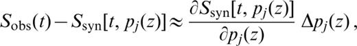
Differential seismograms are used in waveform inversions where a set of seismograms are inverted to estimate the properties of the Earth. The non‐linear relationship between the model parameters and the seismograms is approximated using a first‐order Taylor expansion:

where Sobs(t) is the vector of time samples of the observed seismogram and Ssyn[t, pj(z)] is the vector of time samples of the synthetic seismogram for a reference velocity model, pj(z). In a typical inverse‐modelling study, the computation of the differential seismogram, {∂Ssyn[t, pj(z)]}/[∂pj(z)], is the major burden. In order to reduce the computational cost, most waveform inversion schemes use only phase differentiation to approximate the differential seismogram. This approximation is not adequate as perturbation of the structural model, Δpj(z), can affect the eigenfunctions as well (Stutzmann & Montagner 1993; Kennett 1995; Du & Panza 1998). The development of this analytic technique for the exact calculation of differential seismograms has obvious implications for waveform inversion studies. For example, our differential seismogram method can be easily implemented within the ‘partitioned waveform inversion’ scheme proposed by Nolet (1990), so that not only the perturbation of the phase term but also that of the amplitude term is included in the linearized inversion (Du & Panza 1998). In addition, the speed and the accuracy of the technique may allow for the adoption of Monte Carlo‐derived global search minimization techniques for waveform fitting.
6 Conclusions
We have presented a new analytical technique for the fast and accurate calculation of differential seismograms with respect to medium parameters. The technique adopts the multi‐mode summation formalism (e.g. Panza 1985). Calculation of differential seismograms involves the determination of just one additional mode spectrum, and, depending on the total number of the layers that make up the structural model, it can reduce the computation cost by as much as two orders of magnitude. The technique can be used in waveform inversions for structural parameters within locally linearized, iterative and global search schemes.
Acknowledgements
We would like to thank G. R. Foulger for carefully reading this manuscript and Peter Suhadolc for reading an earlier version of this manuscript and for his suggestions. The thorough review, comments and criticism provided by B. L. N. Kennett, A. Levshin and three anonymous reviewers greatly improved the manuscript. This research has been partially funded through the European Union contracts EV5V‐CT94‐0491, ENV4‐CT96‐0255, ENV4‐CT96‐0296 and through CNR (94.00193.05, 96.00318.05), MURST 40% and 60% funding
The public domain GMT graphics software developed by Wessel & Smith (1991) has been used throughout.
References
Appendices
Appendix A: Partial Derivatives Of Eigenfunctions And Energy Integrals
Following the formulations given by Schwab (1970), Schwab & Knopoff (1972) and Schwab (1984), the evaluation of the partial derivatives of eigenfunctions u(z), w(z), σ(z) and τ (z)is reduced to the determination of the partial derivatives of the layer constants Am, Bm, Cm and Dm (see Schwab 1970) for the layers above the homogeneous half‐space, and the constants An and Bn for the deepest structural unit.
We compute the derivatives of the elements of the (1 × 6) matrix that appears in the basic interface–matrix multiplication of Knopoff’s method (Schwab & Knopoff 1972):

where Ui, Vi, Wi, Ri, Si are the ith interface elements in the fast form of Knopoff’s method for Rayleigh‐wave computation.
For the first interface and a continental structure the elements are as follows:
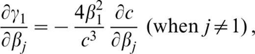
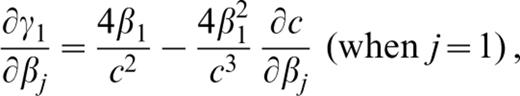
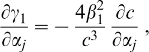
where the derivatives of γ1=2β21/c2, where β1 is the S‐wave velocity in the upper layer, with respect to pj (pj=βj, αj or ρj) are

For the (m+ 1)th layer, the elements in (A1) are the linear combination of their values in the mth layer multiplied by the quantities εk(m) (k=0, 1, … 16) and ζk(m) (k=1, 2, … 15) given in Table 2 of Schwab (1970). We have the following:
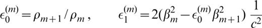
and

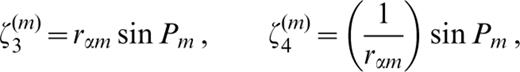
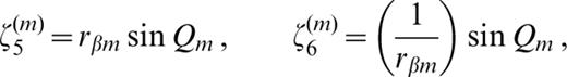
where Pm=dm(ωc/c)rαm, Qm=dm(ωc/c)rβm, dm is the thickness of the mth layer, and rαm and rβm are defined in Schwab (1970).
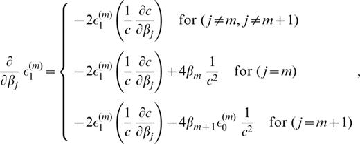
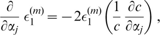
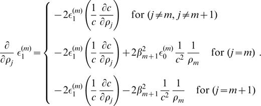
The derivatives of ε1(m) with respect to pj (pj=βj, αj or ρj) are as follows:
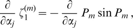
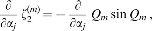
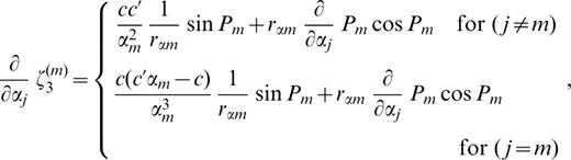
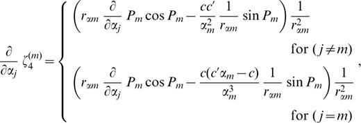
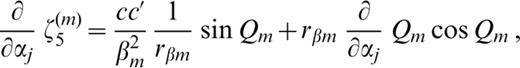
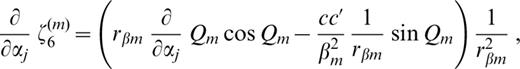
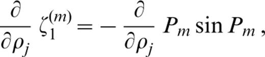
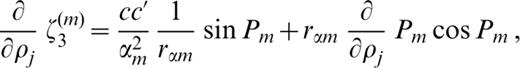
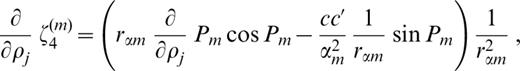
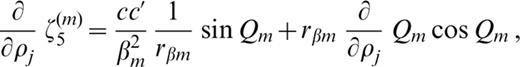
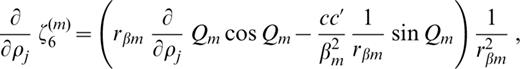
The derivatives of ζk(m) (k=1, 2, … 6) with respect to pj ( pj=βj, αj or ρj) are as follows:
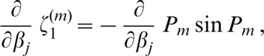
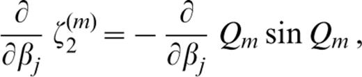
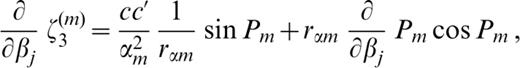
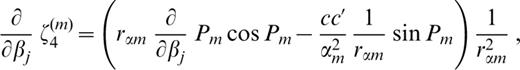
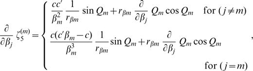
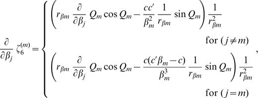
where c′ denotes the derivative of the phase velocity with respect to βj;
where c′ denotes the derivative of the phase velocity with respect to αj;

where c′ denotes the derivative of the phase velocity with respect to ρj.
The derivatives (∂/∂pj)Pm and (∂/∂pj)Qm ( pj=βj, αj or ρj) involved in eqs (A5)–(A7) are as follows:
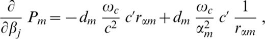

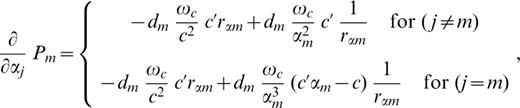
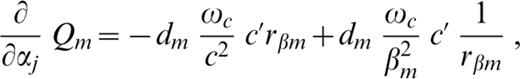
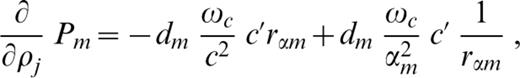
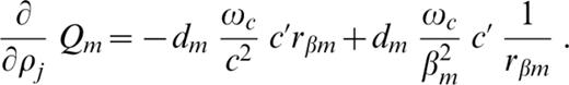
In eqs (A8a) and (A8b) the symbol c′ denotes the derivative of phase velocity with respect to βj, whereas in eqs (A8c) and (A8d) it denotes the derivative with respect to αj, and in eqs (A8e) and (A8f) it denotes the derivative with respect to ρj.
The other derivatives of εk(m) (k>1) and ζk(m) (k>6) can be computed easily from the derivatives of ε0(m) and ε1(m), and ζk(m) (k=1, 2, … 6) [see Table 2 of Schwab (1970)]. This allows us to express the derivatives of the interface‐matrix elements:
(where pj=βj, αj, ρj) for all interfaces down to the half‐space. From eq. (A9), the same procedures used to compute the layer constants Am, Bm, Cm, Dm, An and Bn (Schwab 1970; Schwab 1984) can be used to obtain their derivatives. Finally, from the derivatives of the layer constants, we obtain the derivatives of eigenfunctions, and from eq. (4) we compute the derivatives of the energy integral.
Appendix B: Partial Derivatives Of Group Velocity
The group velocity, u, is equal to the partial derivative of the frequency, ω, with respect to the wavenumber, k:
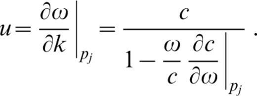
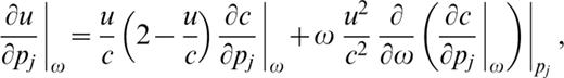
Using the implicit function theory, the partial derivative of group velocity with respect to the model parameter pj ( pj=βj, αj, ρj) can be written as
For a given Rayleigh‐wave mode, the expressions of (∂ ,/∂pj)|ω (Levshin 1989) are
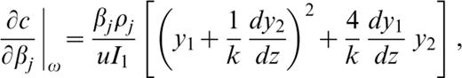
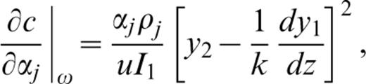
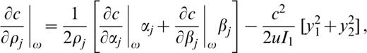
where y1=u(z)/w(0), y2=w(z)/w(0).
The eigenfunctions can be represented through a linear combination of exponential functions (Haskell 1953; Levshin 1989), which, at a given angular frequency, ω, can be written as

Therefore, (∂ ,/∂pj)|ω (eq. B2) is a linear combination of exponential functions.
Exponential function (B4) can be approximated through a series expansion, which, when the argument is small, may correspond to a low‐order polynomium.
In the actual calculations, for each mode we are given the analytical values of (∂c/∂pj)|ω at a discrete number of frequency points, ωl (l=1, 2, …, N), and we choose to approximate locally the derivatives (∂c/∂pj )|ω using a cubic spline polynomium:
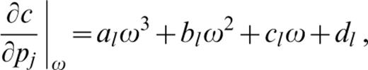
where the coefficients al, bl, cl and dl are determined from (∂c/∂pj)|ω at each frequency, ωl, using the two adjacent frequency values (i.e. ωl− 1 and ωl+ 1) by imposing the smooth‐ness of the first derivative and the continuity of the second derivative both within the interval and at its endpoints (Press 1988). To constrain the interpolation properly, at the two end frequencies of each mode, Rodi et al.’s numerical method is enforced.
In practice, if Δω=ωl−ωl− 1=ωl+ 1−ωl is the frequency interval used in the computation of the spectral quantities, recalling that the maximum value of |rβm| or |rαm| is equal to 1, the error in the calculation of (∂ /∂ω)[(∂c/∂pj)|ω]|pj depends upon the quantity
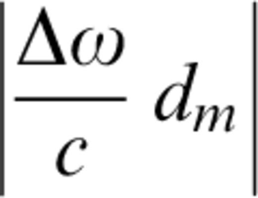
around each frequency point ωl. However, this can be kept reasonably under control by adjusting dm and Δω.
Author notes
Now at: Department of Geological Sciences, University of Durham, Durham, DH1 3LE, UK. E‐mail: [email protected]
Now at: Osservatorio Geofisico Sperimentale, PO Box 2011 Opicina, 34016 Trieste, Italy.
