


Summary
The Archaean paradox stems from the fact that while certain lines of evidence suggest that Archaean continental geotherms were similar to those at present, other lines of evidence suggest that the average mantle heat flux was considerably greater. The simplest qualitative solution, which holds that a greater proportion of heat loss was carried by the creation and subduction of oceanic lithosphere in the Earth’s past, has lacked a clear physical basis. At a fundamental level, it requires that the ratio of mantle heat loss below oceans to that below continents be an increasing function of overall convective vigour and, to date, no self‐consistent model has been used to suggest a means by which this could be so. A simple means is suggested by models that allow accumulations of chemically light near‐surface material, analogues to continents, to form within the upper thermal boundary layer of a thermally convecting and chemically dense fluid, an analogue to the mantle. The physical properties of continental crust cause the thermal coupling condition between a model continent and the convectively unstable mantle below to be different from that which exists at the interface between mantle and oceans. For the latter, a spatially constant temperature condition holds due to (1) the participation of oceanic crust in convective mantle overturn and (2) the large effective thermal conductivity of oceans relative to the mantle. For the former, a spatially near‐constant equilibrium heat flux condition holds due to (1) the long‐term stability of continental crust against remixing into the mantle and (2) the comparable thermal conductivities of distinct rock types. This leads to a laterally variable thermal condition at the surface of the convecting mantle, which, in turn, leads to different local mantle heat flux behaviour in continental versus oceanic regions. As a result, heat flux below continents can increase at a slower rate, with increasing convective vigour, than it does elsewhere. Model heat‐flux scalings are used to assess the degree to which continental geotherms can be time‐stabilized by this means. Results suggest that the thermal surface heterogeneity imposed on the mantle by the presence of continental crust can prevent wide‐scale crustal melting in the Archaean by forcing oceans to carry a greater proportion of the Earth’s heat‐loss load in the past.
Introduction
Various lines of evidence suggest that Archaean continental geotherms were not much different from those occurring at present (Burke & Kidd 1978; England & Bickle 1984; Boyd 1985), yet radiogenic mantle heat production must have been higher, suggesting an average mantle heat flux significantly greater than at present (McKenzie & Weiss 1975; Davies 1980; Richter 1984). Over the years several potential solutions have been offered for the apparent contradiction that arises (Burke & Kidd 1978; Bickle 1978, 1986; Davies 1979; Jarvis & Campbell 1983; Richter 1985; Pollack 1986; Ballard & Pollack 1988). One of the more popular solutions holds that the creation and subduction of oceanic plates carried a greater proportion of the Earth’s heat‐loss load in the Archaean relative to the present. This, it is argued, would allow continental geotherms to remain relatively unchanged over time (Burke & Kidd 1978; Bickle 1978). Such a solution relies on a decline in the ratio of continental to oceanic mantle heat flux as one goes back in time; that is, as the vigour of mantle convection increases. The consistency issue raised by this seemingly straightforward idea was noted some time ago (England & Bickle 1984): no self‐consistent mantle convection model predicts a spatially disproportionate heat loss that is dependent on convective vigour; that is, no physical basis has been provided for an increase in oceanic versus continental mantle heat loss.
The problem most mantle convection models have with the Archaean is expressed by the relatively simple models of Fig. 1. The models are of thermal boundary layer type (Appendix A). The upper thermal boundary layer (TBL) is an analogue for the Earth’s thermal lithosphere. Models of this type, allowing for internal heating as well as added rheological and/or geometrical complexity, have formed the standard model of mantle convection. That is, the majority of self‐consistent models formulated to date have considered mantle convection to be dominantly a TBL phenomenon. The widespread acceptance of TBL models and theory for thermal evolution problems reflects, at its heart, the reason why the Archaean paradox is seen as such. Classical TBL theory and its variants are based on the assumption that the thickness of an upper TBL in a convecting medium thins with increasing convective vigour in the same manner across its lateral extent. Equivalently, the local heat loss out of a convecting layer increases with increasing convective vigour in the same manner, no matter where one is situated above the layer (Turcotte & Oxburgh 1967; Olson & Corcos 1980; Morris & Canright 1984; Solomatov 1995). This lateral homogeneity in the physics of system heat transfer is what allows an essentially 1‐D description, TBL theory, to capture the essence of average heat‐transfer properties in both 2‐ and 3‐D thermal convection experiments and simulations. The problem for the Archaean is that this implies that the ratio of mantle heat loss over any portion of the Earth divided by that over any other portion is independent of convective vigour (Fig. 1).
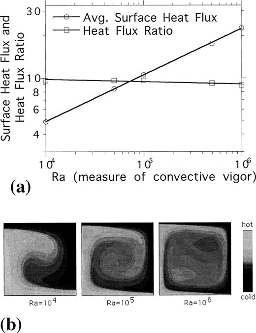
Results from bottom‐heated thermal convection models. (a) Log–log graph showing the Ra dependence of average surface heat flux and the surface heat‐flux ratio for thermal convection models. (b) Steady‐state thermal fields from models with increasing Ra. The heat‐flux ratio is defined as the average heat flux over the left one‐tenth of a model divided by that over the right one‐tenth. Note that unlike average heat flux it is independent of Ra. This is true independently of the spatial averaging extent used to define the heat‐flux ratio (provided the same extent is used over any two portions of the domain). It is also true for internally heated models and models that allow for temperature‐dependent viscosity.
Models that assume that the thickness of continental lithosphere has remained roughly constant over time, due to its high viscosity and/or low density, implicitly assume a spatially disproportionate heat flux that is time‐variable (e.g. Davies 1979; Ballard & Pollack 1988; Nyblade & Pollack 1993). Such models have generally assumed completely rigid continents, which is difficult to reconcile with the fact that continents appear more deformable than oceanic regions (e.g. Vink, Morgan & Zhao 1984; Molnar 1988). It is easy to suggest that only cratonic roots have remained at a constant thickness, but for this to be considered a solution requires self‐consistent modelling to be undertaken to explore the conditions necessary to stabilize thick cratonic lithosphere over geological time (note that this solution avenue implicitly assumes that the majority of issues connected with the Archaean paradox are directly tied to another outstanding problem, the stability of deep continental lithosphere). It seems likely that models exploring the conditions by which thick cratonic lithosphere can be stabilized within a vigourously convecting mantle will need to invoke depleted residuum to form cratonic roots and a means by which residuum can be strong relative to the mantle. This opens a wide parameter space requiring exploration (e.g. Doin, Fleitout & Christensen 1997). For the issue of root stability such an exploration is certainly valuable. However, for the more general issue of the Archaean paradox, it is, to my mind, premature to invoke deep residuum roots before exploring the effects of the more obvious source of lateral surface heterogeneity within the Earth, continental crust.
The advantage of invoking continental crust is that, unlike residuum, its chemical buoyancy is sufficient to keep it from being remixed into the mantle on a large scale. Thus, there is no need to invoke ill‐defined rheological conditions to stabilize crust over time, as seems to be the case for residuum roots. By the same token, as crust is believed to be weaker than mantle any solution involving it cannot be a mechanical one at its core. Rather, it must be thermal. At a primary level the Archaean paradox demands some form of lateral heterogeneity to be present in the Earth’s mantle convection system. Thus, continental crust must introduce a thermal surface heterogeneity to mantle convection that would not be present without it. The rest of this paper sets out to show that (1) continental crust can do this, (2) its presence can cause the ratio of oceanic to continental mantle heat flux to increase into the Earth’s past, and (3) this can stabilize continental geotherms to a degree that the lack of increased crustal melting in the Archaean, in the face of increased mantle heat loss, is not at all paradoxical.
Thermal/Chemical Boundary Layer Models
Models of this section consider mantle convection to be a thermal/chemical boundary layer (TCBL) process. Specifically, the effects of continental crust are not assumed higher order as is the case for TBL models. Models begin with a uniform layer of chemically buoyant ‘crust’ within the upper TBL of a chemically dense and thermally convecting ‘mantle’. Convective stresses cause crust to thicken above mantle convergence zones, thereby forming accumulations that serve as model continents; that is, a continent is considered to be, to first order, an accumulation of chemically buoyant crust that resists wholesale participation in convective mantle overturn. The vigour of thermal convection is controlled by a bottom‐heating Rayleigh number, Ra, and a heating ratio, H, that parametrizes the proportion of internal to bottom heating. For variable‐viscosity models, quoted Ra values are defined at the system base. For this class of models the specific temperature‐dependent viscosity functions used for crust and mantle are also parameters. The ratio of chemical to thermal Rayleigh number, Rac/Ra, parametrizes the strength of chemical to thermal buoyancy forces. Relative crustal volume is represented by the initial uniform depth of the crust, ICD. Total crustal buoyancy depends on both Rac/Ra and ICD. For some models an enrichment of heat‐producing elements in the crust is allowed for and the enrichment factor, HE, becomes an additional parameter. The final control parameter is the size of the modelling domain. A fuller model description is given in Appendix A along with a discussion of solution procedures.
The remainder of this section is divided into two subsections. The first describes the basic mechanism allowing for increased oceanic to continental mantle heat loss with increasing convective vigour. It does so using the simplest of relevant models; that is, those that isolate the essence of the mechanism free from all other potential complexities. The second subsection tests the robustness of the mechanism when other complexities associated with mantle convection are allowed for.
Simple illustrative models
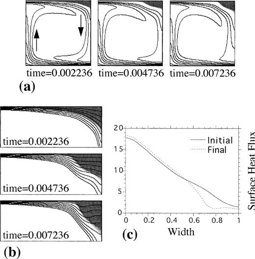
Fig. 2 shows the evolution of a prototype model. After a chemical accumulation forms, its large‐scale morphology changes slowly over time. The essential thing to note is that a constant temperature condition does not hold the base of the accumulation. Rather, the thermal condition is an imperfect one. This implies that both lateral temperature and heat‐flux variations are constrained at the base of the accumulation (Appendix B). That the condition is not one of constant temperature is due to (1) the buoyancy of continental crust keeping it from participating in convective mantle overturn (unlike oceanic crust), (2) the non‐negligible thickness of continental crust relative to thermal lithosphere, and (3) the finite thermal conductivity of crustal rock. Condition (1) allows crustal accumulations to form stable bounding material above the convecting mantle in much the same way as water is bounding material above the convectively overturning portions of the solid Earth in oceanic regions. Conditions (2) and (3) mean that thermal perturbations generated at the base of an accumulation, equivalently at the top of the convecting mantle, by heat loss from below are not rapidly diffused away. Below oceanic regions such perturbations are rapidly smoothed away. These factors cause the convecting mantle to see a laterally variable thermal condition at its surface. Given that the specifics of heat transfer in a convecting system depend on surface conditions, this suggests that heat flux might not increase at the same rate below oceans and continents with increasing convective vigour. Further, in a thermally convecting system an increase in average local heat flux is associated with an increase in the lateral gradient of the heat flux. Thus, locally constraining this gradient can impose a stronger constraint on heat‐flux increase than that associated with a local constraint on temperature.
Evolution of an isoviscous, thermal/chemical boundary layer convection model with Ra=105, H=0, ICD=0.02, and Rac/Ra=2 (this nominal value assumes reference crustal and mantle densities of 2800 and 3300 kg m− 3, a non‐adiabatic temperature drop of 2500 K and a thermal expansion coefficient of 3 × 10− 5 K− 1). (a) Isotherms over composition shade plots for the full model domain (grey shading indicates crust, and isotherms span the hot two‐thirds of the thermal field). (b) Isotherms over composition shade plots for the upper 0.2 of the model domain (isotherms span the cold half of the thermal field). (c) Non‐dimensional surface heat‐flux profiles (the ‘final’ profile is from the last time frame in (a); the ‘initial’ profile is just after model start time).
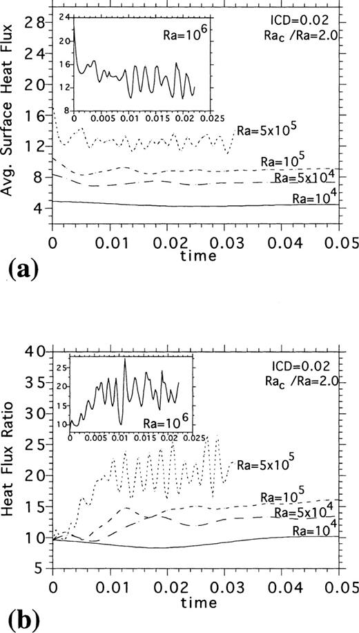
Fig. 3 plots the time evolution of the spatially averaged surface heat flux and a heat‐flux ratio for several models. The heat‐flux :is a measure of average oceanic to continental mantle heat flux; a specific definition facilitates comparisons of TCBL and TBL models (Figs 1 and 3), but results are robust if averages from the full extent of oceanic and continental regions are used to define the ratio, as will be done for multiple‐continent models. As with TBL models, global heat flux increases with Ra. However, for TCBL models the heat‐flux :is also a function of Ra. To show this more clearly, Fig. 4 plots the time‐ and space‐averaged surface heat flux and the time‐averaged heat‐flux ratio versus Ra for several sets of variable ICD models (ICD=0 models are of purely TBL type). Time‐averaging began once model time‐series plateaued to a near‐steady‐state value or to an oscillating state; that is, after the start‐up transient associated with continent formation. Time‐series were averaged using variable windows, and a system was considered to have entered a quasi‐statistically steady state when averages determined from increasing time‐duration windows differed by less than 2–3 per cent.
Time evolution of the average surface heat flux, (a), and the surface heat‐flux ratio, (b), from thermal/chemical boundary layer convection models with ICD=0.02 and variable Ra as noted in the graphs.
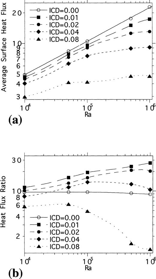
Log–log graphs of the average surface heat flux versus Ra, (a), and the surface heat‐flux ratio versus Ra, (b), for models with variable ICD values.
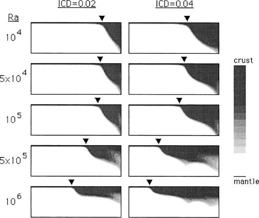
Fig. 4 shows that as ICD is increased, the rate at which average heat flux increases with Ra declines, but the curves maintain a positive slope. Heat‐flux‐ratio curves, on the other hand, roll over at progressively lower Ra as ICD increases. For all model sets, heat‐flux‐ratio rollover is associated with continental extent exceeding one‐half of the modelling domain (Fig. 5). That is, the curves peak as continental extent approaches one‐half the domain size and decrease from this point to the point at which a crustal layer covers the entire model extent. Recall that the thermal condition imposed on the mantle below a crustal accumulation is one of spatially near‐constant heat flux. Thus, if a uniform crustal layer exists, then the heat‐flux :must tend toward unity, which it does.
Composition shade plots over the upper 0.2d of the modelling domain for models with variable ICD and Ra.
That the heat‐flux ratio peaks when the lateral heterogeneity imposed on the mantle by the presence of continents does is somewhat intuitive. Why lateral heterogeneity is a function of Ra relates to the balance of thermal and chemical buoyancy forces within the upper boundary layer. A crustal accumulation is associated with a chemical buoyancy force that makes it want to spread. For local mechanical equilibrium to exist within the model this force is opposed by a thermal buoyancy force that tends to compress an accumulation. The thermal buoyancy force is proportional to the thickness of the thermal boundary layer driving mantle overturn The chemical buoyancy force is proportional to the average thickness of a crustal accumulation. As Ra increases the thickness of the mantle thermal boundary layer decreases and, thus, the average thickness of a model continent must also decrease to maintain equilibrium. For fixed ICD, this leads to increased continental extent. Note that a decrease in negative thermal boundary layer buoyancy with increased Ra, the key to the argument above, implies that changes in Ra are driven principally by changes in viscosity, not by changes in the temperature drop driving the flow. Varying Ra while maintaining fixed Rac/Ra within the model inherently assumes that this is the case (see Appendix A). That it is also likely the case for the Earth has been argued for rather forcefully by Tozer (1972).
For whole‐mantle convection, the lowest ICD model set of Fig. 4 is most relevant. In fact, even lower ICD values than were explored, due to resolution restrictions, are likely for this case. This is important as Fig. 5 suggests that lower ICD values will be required in order for models to generate an ocean–continent dichotomy at very high Ra. For upper‐mantle convection the higher ICD sets can become relevant, suggesting that the heat‐flux ratio may not increase continually in the past. However, this requires that at some point the average extent of continents exceeded the average length of mantle convection cells. This is not the case today, but for layered mantle convection and constant crustal volume over the age of the Earth (Armstrong 1981) it may have been the case in the past. It seems less likely to have been the case in the past if the volume of continental crust increased over time (e.g. Reymer & Schubert 1984).
The main qualitative conclusion of this subsection is that if the average width and length of continents do not exceed the average length of thermal mantle convection cells over Earth history, then the ratio of oceanic to continental heat flux can remain an increasing function of convective mantle vigour. The physical mechanism responsible for this relies on the long‐term survivability and finite conductivity of continental crust. These factors allow continents to introduce a fundamental near‐surface thermal heterogeneity into the Earth’s mantle convection system. On average the thermally convecting mantle sees a relatively constant spatial heat‐flux condition below continents versus the constant temperature condition it sees below oceans. The former is more restrictive to an increase of local mantle heat flux with increasing internal convective vigour and this forces oceanic regions to preferentially carry more heat in the Earth’s past. The next subsection tests the robustness of this conclusion.
Parameter variations
Bottom‐heated, unit aspect ratio convection cells have dominantly been used to develop heat‐flux scalings for TBL convection models. For thermal history modelling this then assumes favourable conditions for convective mantle heat loss over time because (1) bottom‐heated systems lead to higher scaling exponents in heat loss to Rayleigh number relationships than do internally heated systems and (2) unit aspect ratio cells maximize heat loss at a given Rayleigh number (e.g. Christensen 1984). The models of the previous subsection follow this philosophy and further assume that an isoviscous system can provide meaningful physical insight into a specific issue of the Earth’s thermal history. This subsection tests the degree to which these simplifications affect the principal conclusions drawn thus far. This is done through a series of model‐parameter‐variation studies.
Fig. 4 implicitly contains the effects of variable ICD. Heat‐flux decrease with ICD increase reflects the fact that the stable crustal layer absorbs a portion of the temperature drop available to drive convection. The point at which the heat‐flux ratio also becomes a decreasing function of ICD depends on the minimal volume needed to stabilize crustal accumulations from rapid remixing into the mantle. numerical resolution requirements limit the minimum crustal volume that can be represented, and this restricts determination of the ICD point at which long‐lived model continents can be generated. However, the important point is that the heat‐flux ratio can decrease with ICD increase once long‐lived analogues to continents are able to form. Continental growth models show either a constant crustal volume (Armstrong 1981) or an increase over time (e.g. Reymer & Schubert 1984). For the latter, an increase in ICD can be equated with time. Thus, Fig. 4 suggests that crustal growth can add to an oceanic to continental heat‐flux increase in the Earth’s past.
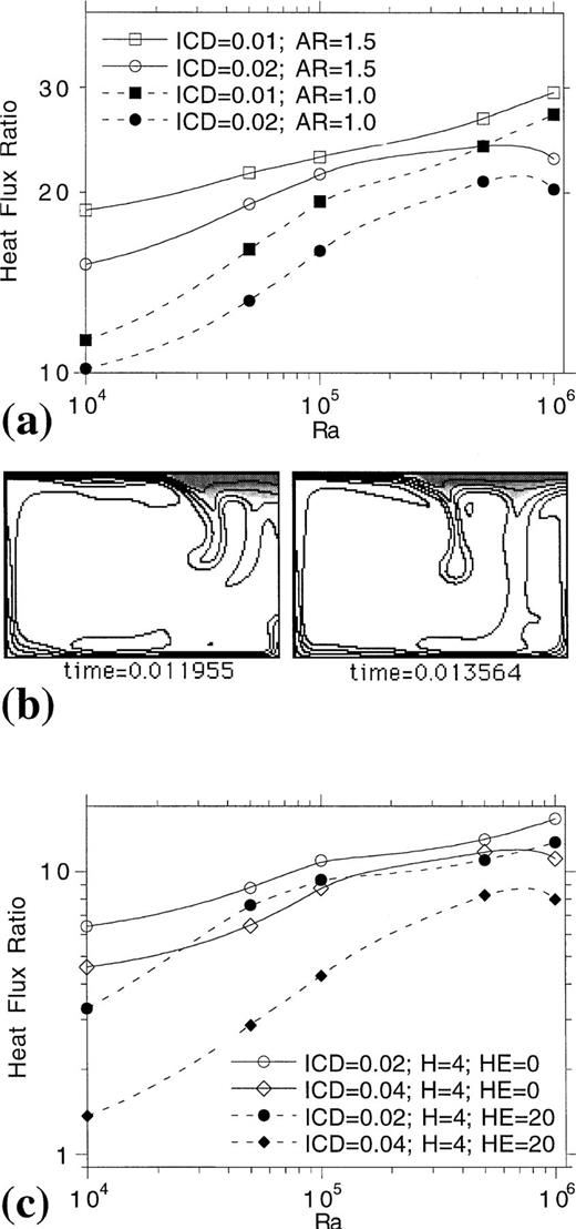
Fig. 6(a) shows the effects of a larger‐aspect‐ratio mantle convection cell. Models with cell aspect ratios ≥ 2 were also explored but for many it was difficult to maintain a single cell within the domain due to continent‐induced splitting events. The laterally variable thermal coupling condition between mantle and stable material above induces large lateral temperature gradients at the edge of a model continent (Fig. 2). As a result, this region can become the site of upper thermal boundary layer instabilities. If the extent of a continent is small, the secondary instabilities are swept to the cell defining thermal downflow before they can penetrate to depth. If the extent is large, then the instabilities can traverse the mantle and deposit cold material at its base. This deflects the lower boundary layer and favours upflow below a continent (Fig. 6b). The cell splitting that results affects subsequent model heat‐transfer properties. These types of events have previously been observed in a different class of models that explored the effects of continents on convection (Gurnis 1988; Lowman & Jarvis 1993). Splitting events were observed for aspect ratio 1 and 1.5 models at higher Ra and ICD. However, for these smaller aspect ratios, cell splitting did not occur rapidly, which allowed average heat‐flux ratios to be obtained over an extended time window for a constant cell aspect ratio. For larger‐aspect‐ratio cases this was not true. This made a full exploration of aspect‐ratio dependence difficult. Fig. 6(a) does, however, suggest that heat‐flux ratio behaviour is not overly sensitive to the convective cell aspect ratio.
Surface heat‐flux ratio versus Ra for models with variable aspect ratios, (a), and for mixed heating models with and without heat enrichment, HE, in the crust, (c).
Fig. 6(c) shows the effects of allowing for internal heating and for a crust enriched in radiogenic elements relative to the mantle (an H value of 4 leads to a mantle dominantly heated from within). Again, heat‐flux‐ratio behaviour remains robust (this was also true for H=8 and 16 models).
The effects of variable Rac/Ra were similar to those of ICD. As Rac/Ra decreased, the depth to which long‐wavelength chemical density variations could be maintained increased and the average extent of a continent decreased. Thus, with decreasing Rac/Ra, the Ra value at which heat‐flux‐ratio curves rolled over increased in much the same way as they did with decreasing ICD (Fig. 4). There was a limit: as for low Rac/Ra and ICD models the chemical buoyancy of continents could not prevent them from being rapidly remixed into the mantle. Models similar to those of Fig. 4 but with Rac/Ra values of 3.0, 2.0, 1.5 and 1.0 were explored. The lower Ra,/Ra classes, with ICD values of 0.02 or less, did not allow continents to be stabilized, and heat‐flux ratios returned to values associated with purely thermal boundary layer models relatively rapidly.
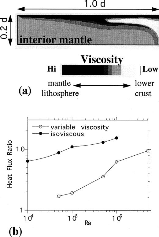
The effects of temperature‐ and composition‐dependent viscosity are shown in Figs 7 and 8. Arrhenius temperature‐dependent viscosities are assigned to crust and mantle. The maximum mantle viscosity drop, from surface to basal temperature, is 104 with a reference value of unity at the base. The viscosity function for crust is of the same form but with a pre‐exponential multiplier, Visr. For Fig. 7Visr=0.01, i.e. crust is 100 times weaker than mantle at equivalent temperatures. This formulation allows for a ‘jelly‐sandwich’ type continental rheology with weak lower crust between strong upper crust and mantle (Fig. 7a). Similarly, the first‐order rheological structure of oceanic regions, with strong lithosphere above interior mantle, is allowed for. Fig. 7(b) shows that these viscosity variations alter heat‐flux‐ratio curves in a quantitative but not qualitative way. Fig. 8(a) shows this further by comparing results from variable ICD and Visr models. Only the models for which the upper boundary layer viscosity was 104 and crust was no weaker than mantle lead to flat heat‐flux‐ratio curves. These models did not allow for the formation of continents as the high viscosity of the upper boundary layer caused it to form a stagnant lid (Solomatov 1995). Without the lubricating effect of a relatively weak crust, to free the upper boundary layer and allow it to overturn (Lenardic & Kaula 1994, 1996), the surface motion needed to cause crustal thickening was absent and model continents could not form. The applicability of stagnant lid models to the Earth is doubtful as they predict no surface motion. It is not the purpose of this paper to suggest that crustal weakness is what allows the mantle lithosphere to participate in convective overturn in the Earth. Models with a weak crust do, however, allow for more Earth‐like behaviour, in that overturning lithosphere can cool the interior mantle, which is the first‐order thermal effect of plate tectonics. Such models remain associated with heat‐flux ratios that increase with Ra provided continents do not take over more than half of the model earth.
(a) Viscosity section over the top 0.2 of the modelling domain from a variable‐viscosity model with Ra=5 × 10⁶, ICD=0.02 and H=4. (b) Heat‐flux ratio versus Ra for isoviscous and variable‐viscosity models with ICD=0.02 and H=4.
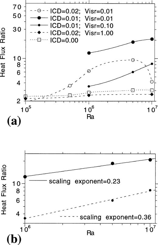
(a) Heat‐flux ratio versus Ra for several variable‐viscosity models with H=4. Crust is Visr× weaker than mantle at equivalent temperatures. (b) Best‐fit power‐law curves for the two ICD=0.01 sets of models from the upper graph.
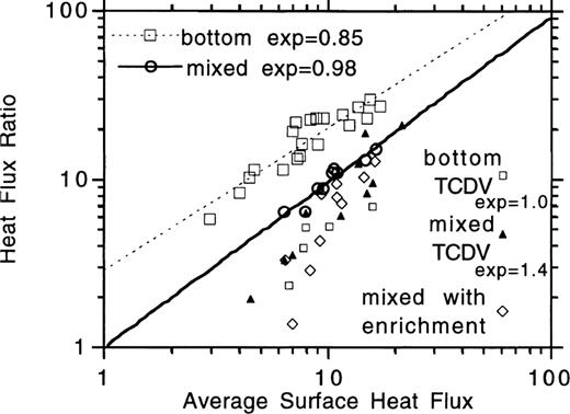
Fig. 8(b) fits power‐law curves onto the heat‐flux ratio versus Ra results from two sets of models (the curves are of the form HFR=Raα, where HFR is the heat‐flux ratio and α is the best‐fit scaling exponent). The results from a variety of models can be plotted in this way but, given that parameters other than Ra vary from model to model, it is better to plot the heat‐flux ratio versus the average surface heat flux (Fig. 9). Power‐law curves are fit onto two subsets of the models to show how model oceanic to continental heat flux can increase with increasing overall mantle heat flux. Curves fitting other sets of models, or all models, led to similar scaling exponents. The bottom‐heated variable‐viscosity models employed a temperature‐dependent mantle viscosity that incorporated a high‐end cut‐off to mimic brittle behaviour. This allowed a greater portion of the upper‐mantle boundary layer to have a high viscosity value (Lenardic & Kaula 1996). The main point to note from Figs 8(b) and 9 is that a variety of models run under variable‐parameter conditions suggest that the ratio of oceanic to continental heat flux can increase as Raα, where an α value of 0.2–0.3 is not at all unreasonable. Similar scalings result if the heat‐flux‐ratio increase is gauged as a function of overall heat loss. The former method is based on models in which only the vigour of convection is increased, that is, on very controlled model sets, while the latter is based on models in which several additional parameters also vary from model to model.
Heat‐flux ratio versus average surface heat flux from a variety of unit‐aspect‐ratio models. Large open squares are results from bottom‐heated isoviscous models, open circles from mixed heating isoviscous models, open diamonds from mixed‐heatingisoviscous models with an enrichment of heat‐producing elements in the crust, small open squares from bottom‐heated temperature‐ and composition‐dependent viscosity models (the exp refers to thebest‐fit power‐law scaling exponent for these model results), and closed triangles from mixed‐heating temperature‐ and composition‐dependent viscosity models. Only models that maintained an average continental extent less than one‐half the width of the modelling domain are plotted.
Controlled models are driven by the fact that many parameters are weakly known, making it wise to isolate their effects before drawing specific conclusions. At times this is not straightforward, which is the case for gauging the effects of multiple continents. Models in wide domains are required and it becomes impossible to maintain constant thermal cell wavelengths. Further, with increasing Ra the number of continents present at any one time can vary from model to model, even for constant crustal volumes. This is due to the fact that such models allow for continental ‘drifting’, ‘splitting’, and ‘colliding’ (Fig. 10). Thus, the effects of these types of behaviour operating collectively in a non‐linear way with each other and with any changes in formal control parameters are what is tested versus the effects of any one in isolation.
Results from a thermal/chemical boundary layer model in a 6 × 1 domain with Ra=106, H=4 and ICD=0.02. Isotherms over composition along with surface heat flux from the full model domain are shown in (a); notice that the top of the image is stretched for visualization. The effects of a drifting chemical accumulation and of colliding chemical accumulations on heat loss are shown, respectively, in (b) and (c), both of which display ≠ar‐surface composition fields along with local surface heat fluxes (model × are shown in the lower right corners of the composition field images).
Fig. 10 shows results from a multiple‐continent model. Note that mantle heat flux can remain spatially near‐constant below continents of variable size and that the average heat flux from continent to continent is also near‐constant (Fig. 10a). For rapidly drifting continents heat flux is not at an equilibrium value; that is, the heat flux out of a crustal accumulation is not necessarily equal to the heat flux into it. On average, however, the mantle heat flux into a drifting continent remains at a near‐constant value. This is because the thermal structure within a drifting crustal accumulation adjusts principally through conduction, the timescale for which is greater than the timescale associated with advective drift. This allows accumulations to ‘carry’ their thermal structure. As they do so, they can induce large lateral thermal gradients at their edges once they drift over warmer mantle (Lenardic & Kaula 1996). This favours the formation of thermal downflows and modulates the thermal conditions below an accumulation. Thus, not only can model continents carry a thermal memory of their origin above downflows, but they can also modulate mantle conditions below themselves to, on average, favour the existence of similar conditions over time. This allows the equilibrium mantle heat flux into an accumulation to remain constant, on average, over time, even when the accumulation itself does not remain in a constant position (Fig. 10b).
During continental splitting events, mantle upflows cause large °s of crustal thinning, and during this time large spatial heat‐flux variations can be generated above a model continent. This happened for example above the initial rightmost continent in Fig. 10(c), which split and began to drift to the left as a thermal upflow rose below it. The local rise in continental heat flux associated with such splitting events, which led to a decrease in the ocean‐to‐continent heat‐flux ratio, was a transient effect as continents that split rapidly drifted off thermal upwellings. Similarly, the change in continental heat flux associated with collisions was also a transient event, as the equilibrium heat flux below a large continent formed from fusion events between two smaller continents tended towards a value similar to that associated with the smaller continents themselves (Fig. 10c).
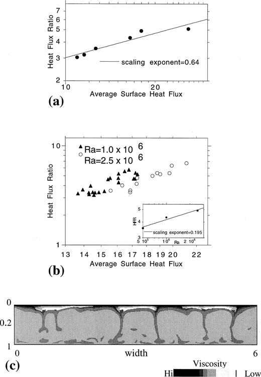
Fig. 11(a) shows the average oceanic‐to‐continental heat‐flux ratio versus the average surface heat flux from several multiple‐continent models. Fig. 11(b) shows how time variations of the heat‐flux ratio correlate with variations in average heat flux from two models, and the inset graph shows how the average heat‐flux ratio scales with Ra for a particular set of models. For any given model, increases in the heat‐flux ratio generally correlate with increases in the average total heat flux (Fig. 11b). This implies that oceanic regions carry most of the added heat associated with pulses of enhanced global heat loss. The exception to this is associated with continental splitting events. Despite these events, the broad trend remains one of correlated heat‐flux and heat‐flux‐ratio increases. The correlation in Fig. 11(b) applies to fast time changes in heat flux, not the secular change associated with a decrease in average surface heat loss; that is, with a decrease in overall convective vigour driven by the decay of radioactive elements in the mantle. The secular correlation for multiple‐continent models is, however, similar to the fast time correlation (Fig. 11a). This was also true for a series of multiple‐continent models that allowed for temperature‐ and composition‐dependent rheology (Fig. 11c shows a representative case from this model set; comparative heat‐flow‐ratio results for multiple‐continent models with and without variable viscosity were similar to those shown in Fig. 7 for single‐continent models).
(a) Average heat‐flux ratio versus average surface heat flux from several 6 × 1 models along with a best‐fit power‐law curve and its associated scaling exponent. From models with highest to lowest average heat‐flux ratios, Ra and ICD values are (1) 5.0 × 10⁶, 0.01; (2) 2.5 × 10⁶, 0.02; (3) 106, 0.02; (4) 5.0 × 10⁵, 0.02; (5) 106, 0.03; and (6) 5.0 × 10⁵, 0.03. For all models H=4. (b) The heat‐flux ratio versus surface heat flux at variable times for two models with ICD=0.02 and variable Ra. For each, values are plotted at a time sampling interval of 0.0002 starting after a model time of 0.005. The inset shows the average heat‐flow ratio versus Ra from models with ICD=0.02 along with a best‐fit power‐law curve and its associated scaling exponent. (c) Log of the viscosity field from a multiple‐continent, variable‐viscosity model (note that, as in Fig. 10, the upper portion of the image is stretched for visualization).
Exploring all the complexities of mantle convection is impractical in the context of a single paper. Thus, although over 150 parameter variations were run, potentially relevant cases remain unexplored. It is worth noting a few of these and the specific assumptions they bring to model application. First, all models were 2‐D. Thus, one must assume that the key behaviour will hold in three dimensions. This seems reasonable as the physical factors key to model heat‐flux behaviour are not geometry‐dependent. Second, the models are limited to Ra≤ 107. Thus, one must assume that extrapolating the results of Fig. 4, for example, to higher Ra and lower ICD values is valid. As model Ra and ICD dependences were smooth for the values explored, this seems reasonable (the possibility of a sharp system transition at high Ra does, however, remain; this would lead to non‐smooth dependences, thereby invalidating extrapolation). Third, no phase changes or depth‐dependent material properties were accounted for. This inherently assumes the effects of such complexities as second order for the specific heat‐flow issue addressed. Fourth, crustal production was not accounted for. Archaean conditions could have lead to increased oceanic crustal production to the point of buoyantly congesting convective overturn of the oceanic lithosphere. Models in this paper rely on such overturn as the principal means of heat loss over Earth history. Thus, one must assume that increased crustal production would not congest the system (delamination could allow for this; Hoffman & Ranalli 1988). Finally, the models do not allow for plate tectonics. For thermal history issues, the principal effect of plate subduction is that it allows cold upper boundary layer material to sink into the deep mantle. Models in this paper also allow for this (rigid‐lid cases being an exception); that is, they are in a free‐lid mode of convection in which the entire mantle thermal boundary layer participates in convective overturn (plate tectonics is also a free‐lid mode of convection but not all free‐lid modes of convection are plate tectonics). The surface motion in the models is of a more distributed form than that associated with oceanic plates. However, recent thermal convection models that allow for self‐consistent plate‐like behaviour lead to heat‐flux scalings effectively equivalent to those for isoviscous convection (Moresi & Solomatov 1998). This implies that what is most important for thermal evolution is that the upper boundary layer participates in convective overturn, not the specifics of its near‐surface velocity and stress profiles; that is, plate‐like versus more distributed free‐lid motion. This offers the promise that principal model results will be robust if plates are incorporated into them. Clearly this and the other assumptions noted need to be tested in future studies.
Discussion And Conclusions
The Archaean paradox initially developed from the lack of evidence of massive crustal melting in the Archaean. The scarcity of minimum‐melting granites in Archaean terrains suggested that temperatures at the base of the Archaean crust did not exceed 800 ° C on average, a value only 300 ° C greater than estimates of the average present temperature (Burke & Kidd 1978). The mild increase in continental geotherms this implied contrasted with the large increase expected based on the greater degree of radioactive heat generation in the Earth during the Archaean, hence the paradox. Burke & Kidd’s (1978) estimates suggested that continental mantle heat flux increased by at most a factor of 1.5 from the present to the Archaean, which, given that global mantle heat flux must have increased by a factor of 4–8 in order to keep pace with internal heat generation (McKenzie & Weiss 1975), suggested to them that oceans carried a greater proportion of heat in the Earth’s past. This suggestion, although generally accepted as reasonable, has lacked a self‐consistent physical basis. The models of the previous section provide such a basis. They show that the buoyant stability and finite thermal conductivity of continental crust impose a laterally variable thermal condition at the top of the convecting mantle. Compared to the con‐stant surface temperature condition seen by convectively overturning portions of the solid Earth in oceanic regions, the imperfect thermal couple between continental crust and convecting mantle provides a greater constraint on the rate at which local mantle heat flux can increase with increasing convective vigour. This forces oceanic regions to carry a progressively increasing proportion of mantle heat loss in the past. The models show that this result is quite robust when various complexities associated with mantle convection (e.g. variable viscosity, mixed heating, drifting continents, etc.) are taken into account. Going beyond this somewhat qualitative conclusion, model results can also quantify the degree to which this mechanism can time‐stabilize the continental mantle heat flux.
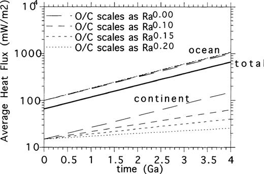
Fig. 12 presents the results from a simple calculation designed to show that the degree of oceanic to continental heat‐flux increase required to prevent Archaean crustal melting can be accounted for by the models of the previous section. The calculation assumes that the thermal Rayleigh number of the bulk mantle increases by an order of magnitude every billion years into the past (Tozer 1972), that the total heat flux depends on the Rayleigh number to the 1/4 power (appropriate for a mantle heated dominantly from within), and that the ratio of oceanic to continental heat flux can also depend on the thermal Rayleigh number to a variable power. The average mantle component of present‐day oceanic heat flux comes from the Pollack, Hurter & Johnson (1993) estimate of oceanic heat flux minus the small contribution due to radioactive decay within the oceanic crust. The average mantle component of present‐day continental heat flux is associated with a greater uncertainty due to our limited direct knowledge about the concentration of radioactive elements in the lower crust. To estimate the equilibrium component of continental mantle heat flux, I have relied on data from the Canadian Shield. This extensive data set is of the highest quality and significant effort has gone into estimating the component of mantle heat associated with it (Pinet et al. 1991; Guillou 1994; Guillou‐Frottier 1995). The cited studies suggest that mantle heat flux ranges from 10–15 mW m− 2 over a wide portion of stable Eastern North America (this includes Proterozoic as well as Archaean terrains). The average total mantle heat flux used in Fig. 12 comes from the estimates of oceanic and continental mantle heat flux above, with 40 per cent of the Earth taken as continental (the ratio of oceanic to continental area is assumed to remain constant into the Archaean, a conservative assumption when it comes to evaluating the degree to which continental geotherms can be stabilized).
Time evolution of average global mantle heat loss and average mantle heat loss in oceanic and continental regions for various degrees of Ra‐dependent heat‐flux partitioning.
Given the estimates of present conditions above, Fig. Fig. 12 shows that if the ratio of oceanic to continental heat flux does not depend on convective vigour, then continental mantle heat flux increases in the past to the point that wide‐scale crustal melting is predicted for the Archaean (Burke & Kidd 1978). This is in essence what most thermal history models based on thermal convection calculations have implied and is one of the main apparent contradictions associated with the Archaean paradox (England & Bickle 1984). Fig. 12 also shows that if the ratio of oceanic to continental heat flux depends on convective vigour in a manner not at all unreasonable based on model results of the previous section (Figs 8, 9 and 11), then Archaean crustal melting can be prevented.
Although the effects of continental crust on mantle convection can clarify aspects of the Archaean paradox, there is still a shortcoming related to diamond inclusion studies (Richardson 1984; Boyd 1985). The problem such data pose is not so much the pressure and temperature conditions they demand in the Archaean continental lithosphere in order to form diamonds (models in this paper can account for this) but that although diamonds formed some 3 Gyr ago they were not erupted with kimberlites until roughly 100 Ma (Boyd 1985). This implies that diamonds remained within the subcrustal lithosphere for a significant portion of the Earth’s history, which in turn implies that portions of the subcrustal lithosphere have been removed from participating in convective mantle overturn for a large period of time. For the models presented, subcrustal lithosphere participates in convective mantle overturn, only the crust does not. Even in models that allow for strong mantle lithosphere (Figs 7 and 8), subcrustal lithosphere overturns just as strong oceanic lithosphere does (the only exception is models in which a fully stagnant lithospheric lid forms, but, as noted, such models face more serious problems in that they do not allow for subduction‐driven mantle cooling). Thus, the models predict that unless diamonds are transported to the crust soon after formation they will be remixed into the mantle along with subcrustal lithosphere within a mantle overturn time; that is, of the order of 108 yr at most. It has been argued that large portions of cratonic lithosphere are transient in this sense and do participate in mantle overturn (Polet & Anderson 1995), but the diamond data suggest that at least some portions do not. This seems to demand that a third chemically distinct component, aside from crust and convecting mantle, be present to provide longevity for portions of the subcrustal lithosphere. Nonetheless, the realization that a small amount of stable crust can have a large effect on mantle convection can go a long way towards clarifying the apparent contradictions associated with the Archaean paradox as a whole. It cannot go all the way as the discussion above notes, but its effects will probably be the key to filling in this last missing piece of the Archaean puzzle.
In conclusion, the presence of continents can introduce a fundamental lateral heterogeneity to mantle convection that favours the preferential increase of oceanic, relative to continental, mantle heat loss in the Earth’s past. The heterogeneity is associated with the finite thermal conductivity of continental crust, which causes the convecting mantle to see a laterally variable thermal condition at its surface. This provides a viable, self‐consistent means by which oceans can be forced to carry more of the Earths heat‐loss load in the past, and it allows continental crust to, in effect, protect itself from wide‐scale melting in the Archaean.
Acknowledgements
This work was supported by the UC Presidents Postdoctoral Fellowship fund. Computing was carried out, in part, at the San Diego Supercomputer Center. I thank S. D. King, A. Raefsky and B. H. Hager for the ConMan finite element code, NCSA Illinois for visualization packages, and Norm Sleep and an anonymous referee for helpful reviews.
References
Appendices
Appendix A: Model Descriptions
Two classes of mantle convection models are discussed in the text, thermal boundary layer (TBL) and thermal/chemical boundary layer (TCBL). Equations defining the TCBL model are presented first. Terms that need to be dropped from the equations in order for them to define the TBL model are then noted.
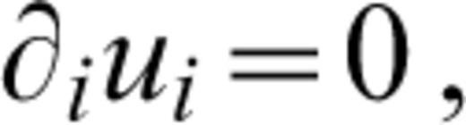
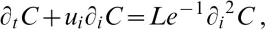
Conservation equations for mass, momentum, energy and composition define the TCBL model. A composition function, C, parametrizes chemical distribution. It is assigned values of 0 and 1 for pure components, which serve as analogues for crust and mantle. Density changes are considered linearly proportional to temperature and composition changes, and are retained only in buoyancy force terms. The model further assumes infinite Prandtl number, a Newtonian viscous rheology that can depend on temperature and composition, negligible shear heating, constant thermal and chemical diffusivity, and no internal composition production or loss. Internal and basal heating and composition‐dependentinternal‐heat‐source density are allowed for. Equations are non‐dimensionalized, scaling length by system depth, d, time by d2/κ, were κ is the thermal diffusivity, velocity by κ/d, temperature by a system temperature drop, ΔT, composition by the maximum compositional variation, ΔC, viscosity by a reference value, μ0, defined at the system base, internal‐heat‐source density by a reference value, Q0, and pressure by κμ0/d2. Non‐dimensional equations for mass, momentum, energy and composition conservation under the stated assumptions, along with a linearized equation of state, are as follows:


where
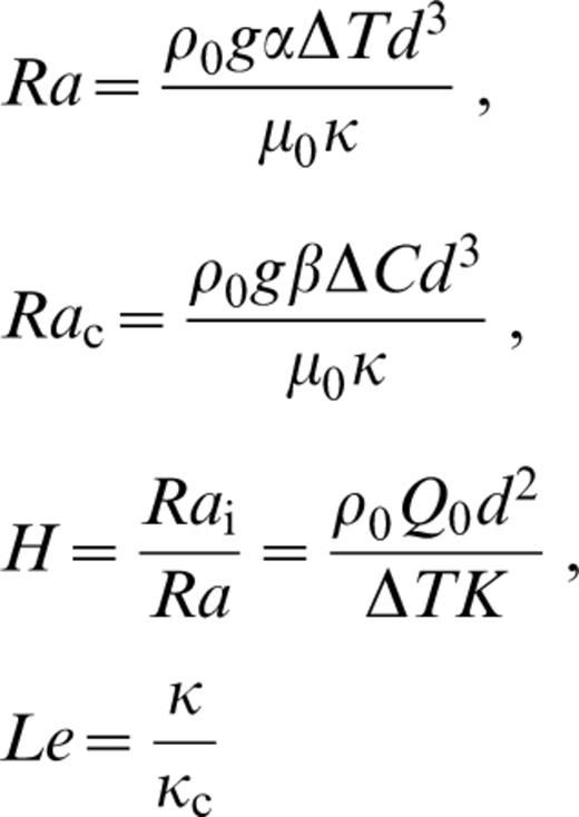
and ui is the velocity vector, μ(T, C) is a temperature‐ and composition‐dependent viscosity function, εij is the strain‐rate tensor, p is pressure, Ra is the thermal Rayleigh number for bottom heating, T is temperature, Rac is the compositional Rayleigh number, {k^ is the vertical unit vector, Q(C) is a composition‐dependent rate of internal heat generation per unit mass, H is the ratio of the thermal Rayleigh number defined for internal heating to that defined for bottom heating, Le is the Lewis number, ρ is density, α is the coefficient of thermal expansion, β is its compositional equivalent, g is gravitational acceleration, Rai is the thermal Rayleigh number defined for internal heating, K is thermal conductivity, and κc is compositional diffusivity.
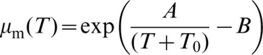
For variable‐viscosity models the non‐dimensional temperature‐dependent viscosity for pure mantle, μm(T), and pure crustal, μc(T), material is given by
and
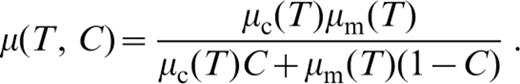
where T0 is a temperature offset set to a value of 0.15, A and B are material constants and Visr is a viscosity ratio less than or equal to unity. These two functions are combined to form a composition‐ and temperature‐dependent viscosity function given by

The TBL model involves only one chemical component that represents mantle. It can be retrieved from the above by retaining eqs (A1), (A2), (A3), (A5) and (A6) and by setting μ(T, C)=μm(T), Rac=0, β=0 and Q(C)=1.
All models have free‐slip horizontal surfaces, reflecting side walls, and a fixed temperature of 0 and 1 on the upper and lower surfaces, respectively. For TCBL models, the upper and lower surfaces are maintained at crustal and mantle compositions, respectively. Initial conditions for TBL models are either a perturbation to the conductive state or thermal fields from lower Ra simulations. The initial thermal field for a TCBL model is obtained by solving a TBL model at equivalent parameter values (for variable‐viscosity models the temperature‐dependent viscosity function of the mantle component is employed). For low Ra cases, the thermal fields are taken to steady state. For cases in which TBL models remain time‐dependent, thermal fields are taken after several convective overturns. The initial chemical field is a thin, uniform‐thickness layer of crust over a deeper mantle layer.
For TBL models, equations are solved using a finite element code (King, Raefsky & Hager 1990). For TCBL models, a modified version of the code is used (Lenardic & Kaula 1993). For simulations in the text, 80 × 80 elements span any 1 × 1 block of a domain. Horizontal resolution is uniform while vertical resolution is enhanced to allow for a local resolution of 0.005 across the upper 0.2 of a domain. Advection of steep composition gradients representing material interfaces in eq. (A4) is treated in two steps. First, a high‐order upwind scheme (Brooks & Hughes 1982) is applied to eq. (A4). Second, a non‐linear filter is applied to remove dispersion errors resulting from advection of steep gradients across fixed grids by minimally dissipative schemes. The filter introduces no diffusion and follows guidelines assuring it will not affect convergence to correct weak solutions (Engquist, Lotstedt & Sjogreen 1989). Despite this, the Eulerian nature of the scheme means that a moving interface cannot be treated as infinitely sharp. This is due to the fact that numerical schemes necessarily treat any subgrid‐scale process as diffusional and in two dimensions there is no way to guarantee that a free interface will fall along grid nodes over all time. This causes an interface to become an interface zone. Physically it means that the interface between components is treated as slightly gradational in a chemical sense, regardless of whether a chemical diffusion term appears in eq. (A4); that is, it will be true for finite and infinite Le.
That interface spreading did not affect the main model results was tested through resolution studies allowing for variable Le and by comparing dynamic thermal/chemical models to semi‐static ones that inserted a fixed block of stable ‘continental crust’ at the top of a convecting ‘mantle’ layer (Lenardic & Kaula 1996). The block was forced to maintain a constant shape such that the interface between it and the mantle remained fixed to grid nodes. Some 40 models of this sort were run with various block shapes, relative block conductivities and convective vigour. As with fully dynamic models, spatial variations of mantle heat flux below the continental block were mild relative to those in ‘oceanic’ regions, provided the block did not have a high thermal conductivity relative to that of the mantle. Further, a decrease in relative block thermal conductivity was associated with an increase in the degree to which the ocean‐to‐continent heat‐flux ratio increased with overall convective vigour (for blocks that approached thermal transparency, i.e. high thermal conductivity, the dependence of the heat‐flux ratio on convective vigour was weak). The disadvantage of applying such models to the Archaean paradox on their own is similar to that noted in the Introduction for models that mimic both shallow and deep continental lithosphere using rigid blocks: a priori assumptions must be made about continental structure over geological time and, given that portions of continents are treated as effectively rigid, ill‐defined rheological assumptions must also be implicitly made. Such models are, however, useful in tandem with more dynamic models (Lenardic 1997) and for addressing ?ions of continent–mantle interaction in which the time‐dependent structure of continental lithosphere is not a primary concern (e.g. Elder 1967; Gurnis 1988; Lowman & Jarvis 1993).
Appendix B: Thermal Coupling
The relative constancy of mantle heat flux below model continents as shown in Fig. 2 is occasionally seen as non‐intuitive. If notions of mantle heat transfer are based on thermal boundary layer models then the result can indeed appear confusing. This is not the case if one recognizes that in thermal/chemical boundary layer systems, of the type explored and argued to be relevant to the Earth, the heat transfer out of a thermally convecting layer does not depend solely on the physical properties and convective state of the layer itself. For the issue at hand, the properties of the convectively stable crustal layer that bounds the mantle from above can have as great an effect on mantle heat transfer as the vigour of thermal convection in the mantle itself. This is most easily shown through a consideration of thermal coupling conditions.
The thermal coupling condition between a convectively unstable layer and material that bounds it from above can be one of locally constant heat flux or constant temperature, or one that lies between the two, often referred to as an imperfect condition (Sparrow, Goldstein & Jonsson 1964). There are various ways of showing how the condition that prevails depends on the relative thermal resistance of the bounding material. A particularly simple way is given below. It follows that of Carrigan (1983), with some additions.
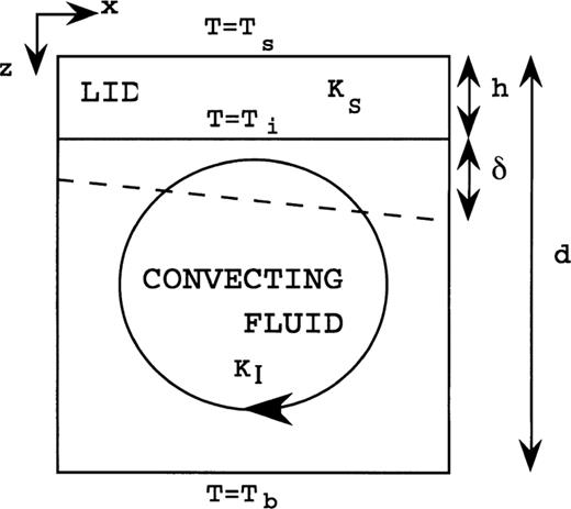
Consider the configuration of Fig. B1. The heat‐flux balance at the interface between the convectively unstable fluid and the material above it is given by

Cartoon of an idealized convective system. The system depth is d, the depth of the stable layer that bounds the convectively unstable fluid layer from above is h, the thermal conductivity of the stable material is KS, the thickness of the upper thermal boundary layer in the convecting fluid layer is δ, the thermal conductivity of the convecting fluid is KI, the surface and basal temperatures are Ts and Tb, respectively, and the temperature at the interface between convecting fluid and the material that bounds it from above is Ti. The discussion in the text assumes that temperature is non‐dimensionalized by the temperature drop across the system so that Ts=0 and Tb=1 and that length scales are non‐dimensionalized by the system depth such that d=1.
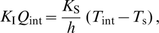
where Qint is defined as the vertical temperature derivative evaluated at the interface. Taking horizontal derivatives and noting that Ts=0 gives
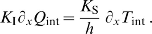
From this the endmember, interface conditions are easily elucidated. If KS≫KI then ∂xQint/∂xTint=∞, so ∂xTint=0. This is the constant‐temperature condition. If KS≪KI then ∂xTint/∂xQint=∞, so ∂xQint=0. This is the constant‐heat‐flux condition.
The magnitude of heat‐flux variations that can result for an imperfect thermal condition can also be elucidated and compared to those that result when a constant temperature is applied to the top of a convecting layer. Consider KS=KI and h=0.1d. Thus, ∂xQint/∂xTint=10. As the temperature of the thermally well‐mixed interior will be near 0.5 for a relatively thin lid, the largest possible ∂xTint is 0.5, implying that the largest possible ∂xQint is 5. Whether this is mild relative to what occurs in the case of a constant‐temperature condition applied at the top of the unstable layer depends on the thermal Rayleigh number. For example, at Ra=105 with constant‐temperature and free‐slip boundaries, a steady 2‐D convection roll in a 1 × 1 domain is associated with a non‐dimensional lateral surface heat‐flux variation of ≈ 18, but at Ra=106 the value increases to 45 (e.g. Blackenbach et al. 1989). Thus, for increasing Ra the imperfect condition approaches a near‐constant heat‐flux condition when viewed relative to a constant‐temperature boundary‐condition case. This Ra dependence is to be expected. The constant‐heat‐flux case implies that the thermal resistance of bounding material dominates surface heat‐transfer properties, with the thermal resistance of the convecting layer playing a lesser role (the extreme case is that of the bounding material being a perfect insulator such that the vigour of convection in the unstable layer has no effect on the transfer of heat out of the layer). The thermal resistance of the convecting fluid depends on its thermal conductivity and the thickness of its upper thermal boundary layer, δ. As Ra increases, δ decreases and, for constant h, the ratio of the resistance to heat transfer in the bounding material to that in the convecting layer increases. Thus, the thermal coupling condition approaches the constant heat‐flux‐case. In fluid dynamics literature this dependence is generally expressed compactly via a Biot number, Bi, defined as the ratio of thermal resistances in bounding and convecting material (e.g. Sparrow 1964; Nield 1968; Chapman, Childress & Proctor 1980). For the case at hand, Bi=(KSδ)/(KIh). For Bi=0 a constant‐heat‐flux equilibrium coupling condition holds. For Bi=∞ a constant‐temperature condition holds. The less compact sketch above shows that even if bounding and convecting material conductivities are equal, the condition at the top of the convecting layer can still be one of relatively constant heat flux when compared to the heat‐flux variations that would result, under similar parameter conditions, if the top of the unstable layer were maintained at constant temperature.
