


Abstract
Many different types of multiparental populations have recently been produced to increase genetic diversity and resolution in QTL mapping. Low-coverage, genotyping-by-sequencing (GBS) technology has become a cost-effective tool in these populations, despite large amounts of missing data in offspring and founders. In this work, we present a general statistical framework for genotype imputation in such experimental crosses from low-coverage GBS data. Generalizing a previously developed hidden Markov model for calculating ancestral origins of offspring DNA, we present an imputation algorithm that does not require parental data and that is applicable to bi- and multiparental populations. Our imputation algorithm allows heterozygosity of parents and offspring as well as error correction in observed genotypes. Further, our approach can combine imputation and genotype calling from sequencing reads, and it also applies to called genotypes from SNP array data. We evaluate our imputation algorithm by simulated and real data sets in four different types of populations: the F2, the advanced intercross recombinant inbred lines, the multiparent advanced generation intercross, and the cross-pollinated population. Because our approach uses marker data and population design information efficiently, the comparisons with previous approaches show that our imputation is accurate at even very low () sequencing depth, in addition to having accurate genotype phasing and error detection.
GENOTYPE imputation describes the process of imputing missing genotypes in study individuals, most often using a high density reference panel of genotypes. For human populations, HapMap (International HapMap Consortium et al. 2007) and the 1000 Genomes Project (1000 Genomes Project Consortium et al. 2012) provide reference panels including millions of SNPs. Genotype imputation has become a key step in the genome-wide association studies of human populations to increase the power of QTL detection and to facilitate meta-analyses of studies at different sets of SNPs (Li and Freudenberg 2009; Marchini and Howie 2010).
Genotype imputation leverages haplotype sharing between study individuals and reference panels. Along chromosomes, the pattern of haplotype sharing changes due to historical recombination. A crucial component of most genotype-imputation methods is to infer the local haplotype clustering and the ancestral haplotypes from reference panels and study individuals (Howie et al. 2009; Li et al. 2010; Browning and Browning 2016). The accuracy of imputation depends on how well reference panels match study individuals in terms of ancestral haplotypes (Pei et al. 2008; Roshyara et al. 2016).
Next-generation sequencing technology has become an attractive and cost-effective tool for QTL mapping in nonhuman populations (Spindel et al. 2013; Heffelfinger et al. 2014; Kim et al. 2016), and genotype imputation is essential for low-coverage sequencing. The focus of this article is on experimentally designed populations, particularly for plants, where study individuals are produced by multigenerational crossing from two or more founders. Many such multiparental populations have recently been created (e.g., Kover et al. 2009; Bandillo et al. 2013; Mackay et al. 2014; Sannemann et al. 2015), aiming at increasing genetic diversity due to many founders and QTL mapping resolution due to accumulated recombination break points over multiple generations.
The founders of multiparental populations are naturally used as the reference panel for genotype imputation. However, there are typically many missing founder genotypes, particularly when both founders and offspring are genotyped by low-coverage sequencing, and some of the founders may even be missing completely (Thépot et al. 2015). In such cases, the population-based imputation methods (Howie et al. 2009; Li et al. 2010; Browning and Browning 2016) are not optimal. Alternatively, pedigree-based genotype imputation methods (Abecasis et al. 2002; Cheung et al. 2013) are computationally intensive, if not impossible, because of the large breeding pedigree being often partially or wholly unavailable and most or all genotypes being missing in intermediate generations.
Recently, several imputation methods were proposed for experimental crosses. Xie et al. (2010) described a parent-independent genotyping method for two-way recombinant inbred lines (RILs), where parental genotypes were obtained using a maximum parsimony of recombination. Swarts et al. (2014) described a Full-Sib Family Haplotype Imputation (FSFHap) method for biparental populations, where parental haplotypes were identified by a custom clustering method over nonoverlapping windows with a window size of 50 loci along chromosomes. Fragoso et al. (2016) described a Low-Coverage Biallelic Impute (LB-Impute) algorithm for biparental populations, where parental genotypes were imputed only after offspring genotypes were imputed using a modified Viterbi algorithm over a sliding window (of size 7 loci) along chromosomes. See also Hickey et al. (2015) for genotype imputation in biparental populations in plant breeding.
In experimental crosses, genotype-imputation methods have mainly focused on biparental populations. There remain challenges for more complicated experimental designs. Huang et al. (2014) described a genotype-imputation method called mpimpute, which is however restricted to the funnel-scheme of four- or eight-way RILs. In the funnel scheme, the founders of each line are randomly permuted. In this article, we present a general statistical framework of genotype imputation from low-coverage GBS data, applicable to many scenarios in experimental crosses. First, it applies to both bi- and multiparental populations. Second, it is parent independent so that it applies even if some founders’ genotypes are not available. Third, it integrates with parental phasing and thus applies to mapping populations with outbred founders. Last but not least, it integrates with genotype calling to account for the uncertainties in identifying heterozygous genotypes due to low read numbers.
Our imputation algorithm is called magicImpute, building on a hidden Markov model (HMM) framework that extends our previous work (Zheng et al. 2014, 2015; Zheng 2015; Zheng et al. 2018). We first evaluate magicImpute with simulated data in four populations: the F2, the advanced intercross recombinant inbred line (AI-RIL), the funnel scheme eight-way RILs, and the cross-pollinated (CP). We then analyze four sets of real data: the maize F2 (Elshire et al. 2011), the maize AI-RIL (Heffelfinger et al. 2014), the rice multiparent advanced generation intercross (MAGIC) (Bandillo et al. 2013), and the apple CP (Gardner et al. 2014). The term MAGIC has been used for many different types of breeding designs, and the rice MAGIC is essentially a set of funnel scheme eight-way RILs (Bandillo et al. 2013). In the evaluations by simulation and real data, we perform comparisons among magicImpute, Beagle version 4.1 (Browning and Browning 2016), LB-Impute (Fragoso et al. 2016), and mpimpute (Huang et al. 2014); investigating, among other things, how imputation quality depends on amount of missing data, level of homozygosity, and coverage of sequencing.
Methods
Overview of model
Consider a mapping population derived from a number of founders. We assume that linkage groups (chromosomes) are independent and thus consider only one group. The genotypic data matrix of sampled offspring is denoted by with element representing the genotype at locus t in offspring i. The founder genotype matrix is denoted by with element being the genotypes at locus t in all founders. We consider only biallelic markers and denote the two alleles by 1 and 2. We model either the called genotypes from SNP array or GBS data, or the allelic depths of GBS data. The called, unphased genotype at a locus can take one of six possible values: 11, 12, 22, or where U denotes an uncertainty allele. For allelic depth data, the genotype is measured by read counts for each of two alleles. The ordering and genetic locations of markers are assumed to be known.
We build an integrated HMM for the genotypic data and but impute missing founder genotypes and missing offspring genotypes separately. The imputation diagram and the overview of the HMM are shown in Figure 1. Here, the hidden founder haplotype matrix where element is similar to except that it contains information on missing genotypes and genotype phases at locus t in founders. See an example in the following section on The genotype model. Conditional on estimated the genotypic data for each offspring are analyzed independently by a sub-HMM, with being the hidden ancestral origin state at locus t in offspring i. The HMM will be further explained in The process model. See Table 1 for a list of symbols and their brief explanations.
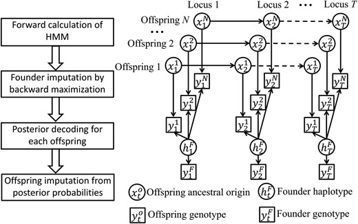
Overview of the imputation algorithm. The left panel shows the diagram of magicImpute. The right panel shows the directed acyclic graph of the HMM for N offspring at T loci, where the arrows denote probabilistic relationships that are described in the Methods section. See Table 1 for the symbols in the right panel. In the left panel, the second step of founder imputation results in the estimate of and the third step of posterior decoding results in the posterior probability of conditional on genotypic data and for and
List of symbols and their brief descriptions
| Symbol | Description |
|---|---|
| Number of founders | |
| N | Number of offspring |
| T | Number of markers (loci) |
| Hidden founder haplotype at locus t | |
| Hidden founder haplotype matrix | |
| Hidden ancestral origins at locus t in offspring i | |
| on maternally (m) or paternally (p) derived chromosome | |
| Genotype at locus t in offspring i that is completely determined by and | |
| Hidden true genotype at locus t in offspring i | |
| Observed genotype at locus t in offspring i | |
| Observed offspring genotype matrix | |
| Observed genotypes for all founders at locus t | |
| Observed founder genotype matrix | |
| Genotypes containing uncertain allele U | |
| Number of reads for alleles 1 or 2 | |
| Allelic error probability for offspring, independent of read depths | |
| Allelic error probability for founders, independent of read depths | |
| Phred quality score | |
| ε | Sequencing error probability |
| Prior probability of at locus 1 in offspring i | |
| Prior transition probability from to | |
| likelihood at locus t in offspring i | |
| Posterior probability of conditional on and genotypic data from loci 1 to t | |
| Unnormalized conditional posterior probability of | |
| Posterior probability of conditional on genotypic data from loci 1 to t | |
| Hats denote maximum likelihood estimates | |
| Single genotype call if probability of most probable genotype is greater than threshold | |
| Impute if probability of most probable genotype is greater than threshold | |
| Correct if probability of most probable genotype is greater than threshold |
The genotype model
Called genotype:
The genotype model corresponds to the vertical relationships (arrows) in the directed acyclic graph of the HMM (Figure 1). Since the genotypes are independent conditional on the hidden states, we consider a single locus t. We first model the prior probability which is assumed to follow a discrete uniform distribution over all possible combinations under the constraint of called parental genotypes Consider an example of four inbred founders with genotypes at locus t denoted by 11, 22, and respectively. We use as a shorthand for the four homozygous genotypes. Then, can take one of four possible values 1211, 1212, 1221, or 1222 with equal probability. Consider the second example of a CP population and the genotypes of two outbred parents which are denoted by 12 and can then take one of eight possible values, 1211, 1212, 1221, 1222, 2111, 2112, 2121, and 2122, where the last four values account for the alternative phase of the first parent’s genotype. The founder haplotype matrix is known if all parental genotypes are observed and phased.
Allelic depth:
Single genotype calling:
The process model
The process model corresponds to the horizontal relationships (arrows) in the directed acyclic graph of the HMM (Figure 1). It has been described in detail (Zheng et al. 2014, 2015; Zheng 2015) and we give a brief summary in the following. The process for offspring i describes how the ancestral origins change along chromosomes. At a locus t, let be the ancestral origins on the maternally (m) and paternally (p) derived chromosomes. If offspring i is fully inbred, we have so that the ancestral origin process along the maternally derived chromosome is the same as the process along the paternally derived chromosome, and it is thus termed “depModel.” On the other hand, if offspring i is completely outbred, the ancestral origin process along the maternally derived chromosome is independent of the process along the paternally derived chromosome, and it is therefore termed “indepModel.” In the general model called “jointModel,” and are modeled jointly. We have kept the model terms (e.g., “jointModel”) consistent with Zheng et al. (2015).
In all three models, the ancestral origin process along two chromosomes is assumed to follow a Markov process, so that the ancestral origins at locus t depends only on at locus but not on the previous Thus, the joint prior distribution of can be specified by the initial distribution and the transition probability at The initial distribution is specified by the stationary distribution of the Markov process, so that the prior process model does not depend on the direction of chromosomes. The initial distribution and transition probability can be specified from the breeding design of a mapping population, that is, how the sampled offspring is produced from the founders; the transition probability also depends on intermarker distances. See Zheng et al. (2014); Zheng (2015); and C. Zheng, M. P. Boer, and F. A. van Eeuwijk, unpublished results, for the details of calculating and under various breeding designs.
Founder imputation
Because the state space of the HMM exponentially increases with the number N of sampled offspring, the exact inference of the founder haplotype matrix is computationally intractable, even using the forward–backward algorithm (Rabiner 1989). In the following, we describe an approximate forward–backward procedure for maximum likelihood estimation of Our forward algorithm calculates recursively the posterior probabilities and for offspring conditional on genotypic data up to locus t. It proceeds as follows:
Algorithm A.
The maximum likelihood estimation of founder haplotypes is based on the posterior probabilities and from Algorithm A. The maximization proceeds backwardly as follows:
Algorithm B.
B0. Initialize at and for
Preliminary simulations showed that our forward–backward procedure is occasionally less accurate on the left end of chromosomes in cases of sparse data. We overcome this problem by two rounds of maximization. Specifically, we fix the founder haplotypes on the right-half chromosomes () after the first round of maximization and then perform the second round with reversed chromosome direction.
Offspring imputation
Conditional on the imputed founder haplotype matrix all the offspring are independent. For each offspring, we first perform the posterior decoding algorithm to calculate the posterior probabilities of ancestral origins at all loci (Rabiner 1989; Zheng et al. 2015). We then calculate the posterior probabilities of true genotypes, from which missing genotypes can be imputed.
From the marginal posterior probability we perform both imputation and error detection for offspring i. For imputation, the missing genotype in offspring i at locus t is imputed to be if its marginal posterior probability is larger than a given threshold . For error detection, the observed called genotype is corrected if the most probable genotype is different from and the maximal marginal posterior probability is larger than a given threshold
Data simulation
We simulate sequence data, mimicking real data in the following mapping populations: the AI-RIL, the F2, the MAGIC (funnel scheme eight-way RIL), and the CP. These populations differ in the number of founders and the heterozygosity level of founders and offspring (Table 2). For each type of mapping population, we simulate independently three sample sizes: 100, 200, and 500, that is, the number of sampled offspring in the last generation. Independently for each type of population with a given sample size, we first simulate the breeding pedigree according to the corresponding real data. The AI-RIL consists of five generations of random mating starting from the F1 generation and six generations of selfing; the size of the random mating population is set to 1000. For each offspring of the MAGIC, the founders are randomly permuted so that the number of funnels equals the sample size.
The running time (in seconds) of genotype imputation for the four real data sets
| Population | Maize AI-RIL | Maize F2 | Rice MAGIC | Apple CP |
|---|---|---|---|---|
| Number of SNPs | 13,912 | 127,059 | 37,240 | 13,493 |
| Founder type | Inbred | Inbred | Inbred | Outbred |
| Offspring type | Inbred | Outbred | Inbred | Outbred |
| Number of founders | 2 | 2 | 8 | 2 |
| Number of offspring | 275 | 87 | 178 | 87 |
| magicImpute | 784 | 212 | 3170 | 627 |
| Beagle version 4.1 | 178 | 31 | 445 | 39 |
| LB-Impute | 3698 | 3579 | NA | NA |
| mpimpute | NA | NA | 406 | NA |
Given a breeding pedigree for each mapping population, we assign a unique founder genome label (FGL) to each inbred founder or to the haploid gamete of each outbred founder. We simulate only one linkage group. Each offspring gamete is a random mosaic of FGL blocks determined by chromosomal crossovers between two parental chromosomes. The number of crossovers in a gamete follows a Poisson distribution with mean being the chromosome length in morgan, and the positions of crossovers are uniformly distributed across the chromosome. We set true founder haplotypes based on the founders imputed from the available real data (see Table 2) and obtain the true offspring genotypes by replacing FGLs with the true founder haplotypes. We apply the same error model to the true founder haplotypes with and to the true offspring genotypes with
We simulate read count data for each obtained founder or offspring genotype. Independently for each allele of a genotype, the number of reads is assumed to follow an exponential distribution with mean being λ/2, where we set the number of erroneous reads follow a binomial distribution with probability and the erroneous read corresponds to the alternative allele. The allelic depths of genotypes are obtained by combining reads of the two alleles. The allelic depths of founder and offspring genotypes are reset to be missing with probabilities 0.25 and 0.15, respectively. We obtain 12 full data sets, three population sizes for each of the four mapping populations, with average offspring read depth 6.8. To study the dependence of sequencing coverage, we retain the same founder reads and randomly sample offspring reads with probability for resulting in a total of 132 test data sets.
Real data
Table 2 shows a summary of real data after filtering. For the maize AI-RIL (Heffelfinger et al. 2014) and the maize F2 (Elshire et al. 2011), we use the GBS data that have been prepared by Fragoso et al. (2016) as the input data of LB-Impute. For the rice MAGIC (Bandillo et al. 2013), we use the called genotypes that have been prepared by Huang et al. (2014) for mpimpute. For the apple CP (Gardner et al. 2014), we filter the original allelic depth data by removing markers with the missing fraction of called genotypes >50% and by removing markers with segregation distortion at significant level of 0.01. During the filtering process, a single genotype is called with threshold and 0.95 for founders and offspring, respectively, as described in the previous section on Single genotype calling. The quality score is set to so that the sequencing error probability
To calculate imputation accuracy, we mask a subset of high-confidence genotypes and use them as the pseudotrue genotypes. For the GBS data, the genotypes are first called with a very large threshold and the quality scores being 30 and 40 for apple and maize, respectively. The called genotypes (excluding and ) are masked with probability being 0.25 and 0.05 for founders and offspring, respectively. After masking, the fractions of founder genotypes without reads are 0.23, 0.24, and 0.19 for the maize AI-RIL, the maize F2, and the apple CP, respectively. The fractions of offspring genotypes without reads are 0.77, 0.16, and 0.095. For each of the three masked full data sets, we retain the same founder reads and randomly sample offspring reads with probability for resulting in 33 real sequencing data sets. For the called genotypes of the rice MAGIC, the missing fraction of founder genotypes after masking is 0.3. From this masked data set, five data sets are produced independently by masking called offspring genotypes to give missing fractions from 0.5 to 0.9 at step size 0.1.
Algorithm evaluation
To set up the algorithm magicImpute, we perform sensitivity analysis of and For each mapping population with size 200 and read depth 0.85, we impute the simulated data set with the input data being called genotypes and the first two founders’ genotypes being not available. By default, we set and the input genotypes are called from allelic depths with threshold and 0.95 for founders and offspring, respectively. Supplemental Material, Figure S1 and Figure S2 show that the accuracies of imputation and error detection increase slightly with from 0.6 to 0.95, while the fractions of imputation and error detection decrease slightly. Figure S1 and Figure S2 also show that the performances of imputation and error detection often become a bit worse when increases by a factor of 10. The effects of these parameters are marginal in general. Thus we set somewhat arbitrarily and in the following evaluations. The algorithm magicImpute also outputs the posterior probabilities of all possible genotypes for all offspring at all markers, from which we can perform imputation and error detection with different and
We evaluate magicImpute by both simulated and real data in the four types of mapping populations. For each of the simulated data sets and the real GBS data sets, we run magicImpute in the four combinations: the first two founders’ genotypes are available or not, and the input data are allelic depths or called genotypes. Here the quality scores are 30 for the simulated data and the real maize GBS data, and 40 for the real apple GBS data. For the real rice data, we run magicImpute in the two combinations: the first two founders’ genotypes are available or not. Results of magicImpute are compared with those of Beagle version 4.1 in all populations. We run Beagle version 4.1 for the called genotypes in two ways: without reference panels and using the founder haplotypes imputed by magicImpute as the reference panels. Additionally, we run LB-Impute for the biparental populations AI-RIL and F2 with the input data being allelic depths, and run mpimpute for the MAGIC population with the input data being called genotypes. LB-Impute and mpimpute do not work if some founders’ genotypes are not available. The running settings of magicImpute, Beagle version 4.1, LB-Impute, and mpimpute are described in File S1. See Swarts et al. (2014) and Fragoso et al. (2016) for comparisons of FSFHap with Beagle and LB-Impute.
Data availability
The algorithm magicImpute is implemented in Mathematica 11.0 (Wolfram Research Inc. 2016) and it has been included as a function in the RABBIT software. RABBIT is available at https://github.com/chaozhi/RABBIT.git and it is offered under the GNU Affero general public license, version 3 (AGPL-3.0). Example scripts for simulating genotypic data are included. The real maize AI-RIL and F2 data have been described by Heffelfinger et al. (2014) and Elshire et al. (2011), respectively, and they have been prepared by Fragoso et al. (2016) for LB-Impute. The rice MAGIC data have been described by Bandillo et al. (2013) and they have been prepared by Huang et al. (2014) for mpimpute. The apple CP data are available from Gardner et al. (2014). Supplemental material available at Figshare: https://doi.org/10.25386/genetics.6854933.
Results
Simulation evaluation
Figure 2, Figure 3, Figure 4, Figure S3, Figure S4, Figure S5, Figure S6, and Figure S7 show the comparisons among magicImpute, Beagle, LB-Impute, and mpimpute in terms of imputation accuracy, error detection, and genotype phasing. All results are obtained from the simulated populations of size 200, except Figure S4 that shows the effects of population size.

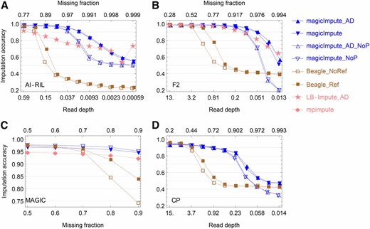
Simulation evaluation on the accuracy of imputing offspring genotypes. (A–D) The results for the AI-RIL, the F2, the MAGIC, and the CP, respectively, are shown. In the figure legend on the right side, “_AD” denotes that the input data are allelic depths rather than called genotypes, “_NoP” denotes that the first two founders’ genotypes are not available, and “_Ref” and “_NoRef” denotes whether Beagle uses founder haplotypes as reference panels or not. When the input data are called genotypes, complete homozygosity is assumed for the AI-RIL and the MAGIC, and thus their missing fractions on the top axes are smaller than those of the F2 and the CP at the same depths.
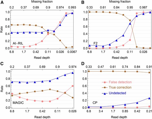
Simulation evaluation on the error detection in offspring genotypes. (A–D) Shown are the results for the AI-RIL, the F2, the MAGIC, and the CP, respectively, which are obtained by magicImpute with the first two founders’ genotypes being unavailable and the input data being called genotypes. The false detection rate (●) denotes the percentage of estimated suspicious genotype errors being not true errors, the true correction rate (▪) denotes the percentage of estimated suspicious genotype errors being true and being corrected into the true genotypes, and the undetected rate (▴) denotes the percentage of true genotype errors being undetected.
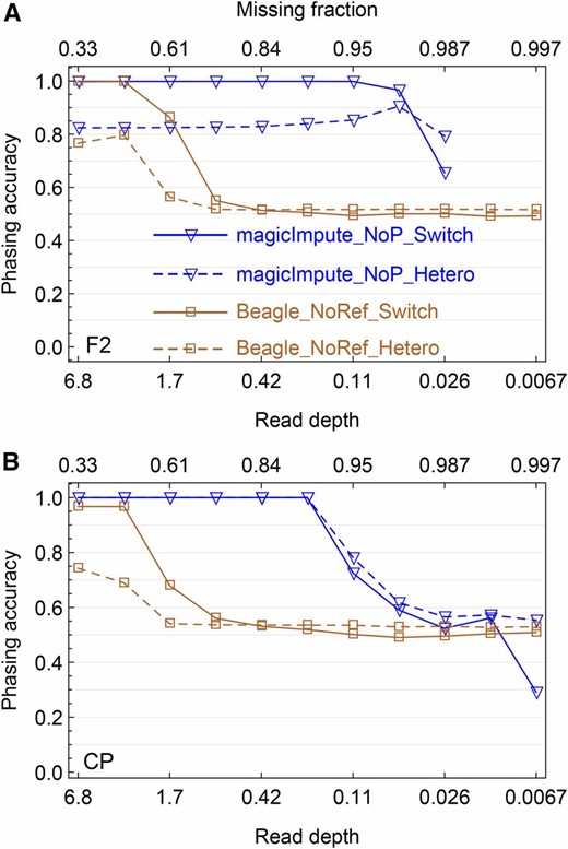
Simulation evaluation on the offspring genotype phasing. (A and B) The results obtained by magicImpute and Beagle for the F2 and the CP, respectively, are shown. For magicImpute, the first two founders’ genotypes are unavailable (_NoP) and for Beagle there are no reference panels (_NoRef). The solid lines denote the switch accuracy (_Switch), one minus the percentage of switch errors to obtain the true haplotype phase; the dashed lines denote the percentage of correctly phased heterozygous genotypes (_Hetero).
Imputation accuracy:
Figure 2 and Figure S3 show the comparisons of imputation accuracy. One of the most striking patterns is that there are break points for magicImpute and Beagle but not for LB-Impute and mpimpute. As shown in Figure 2 for the imputation accuracy of offspring genotypes, the break points of magicImpute are 0.053, 0.11, 0.21, and 0.21 read depth for the AI-RIL, the F2, the MAGIC, and the CP, respectively; much lower than the break points of 0.42, 3.4, 0.85, and 3.4 read depth for Beagle. As shown in the left panels of Figure S3, the break points of magicImpute for founder imputation are the same as those for offspring imputation; Beagle does not impute founder genotypes.
As for mpimpute and LB-Impute, they perform slightly worse than magicImpute. The imputation accuracy of mpimpute is ∼1.7% lower than that of magicImpute when read depth >0.21 (Figure 2C). The imputation accuracies of LB-Impute at the highest read depth are similar to those of magicImpute, but they decrease gradually with decreasing read depth. In addition, the imputation fractions of LB-Impute at the highest read depth are ∼0.8, much smaller than those of magicImpute (Figure S3, B and D).
The unavailability of the first two founders’ genotypes has no noticeable effects on the performance of magicImpute for the AI-RIL, the F2, and the MAGIC, as long as read depth is higher than the break point. However, for the CP, the availability of the two outbred founders’ genotypes results in ∼2% lower accuracy of imputing founder genotypes (Figure S3G) due to the calling errors in the available founder genotypes. As a result, the imputation accuracy of offspring genotypes is ∼4% lower (Figure 2D).
Whether the input data are allelic depths or called genotypes has little influence on the performance of magicImpute. However, for the almost homozygous populations AI-RIL and MAGIC, the ceiling limit of imputation accuracy decreases with increasing read depth instead of leveling off (Figure 2, A and C). This is due to the assumption of homozygosity during the prior genotype calling and the information on residual heterozygosity is lost after transforming allelic depths into called genotypes. The percentage of heterozygotes among missing genotypes increases with increasing read depth and they are always missing and wrongly imputed.
Figure S4 shows that the main effect of population size is shifting the break points of the imputation accuracy obtained by magicImpute and Beagle.
Error detection:
We evaluate the error detection of magicImpute in the case of the input data being called genotypes. A suspicious genotype error is detected by magicImpute when the most-probable true genotype is different from the input called genotype and the maximum posterior probability is larger than the default threshold As shown in Figure 3 and Figure S5, the unavailability of the first two founders’ genotypes greatly improve the error detections for the F2, the CP, and the AI-RIL, but it has little effects on the MAGIC with multiple founders. This indicates that the errors in the available founder genotypes adversely affect the detection of offspring genotypes.
Figure 3 and Figure S5 show that the error detection in the almost homozygous populations AI-RIL and the MAGIC is much worse than in the F2 and the CP. This is due to the homozygosity assumption under which the input genotypes are being called for the AI-RIL and the MAGIC; most offspring genotype errors are heterozygous and they cannot be detected and corrected when the heterozygosity information is lost during the prior genotype calling. Figure S6 shows that the error detection in the AI-RIL and the MAGIC is much better when homozygosity is not assumed.
Genotype phasing:
We evaluate the phasing accuracy for the heterozygous populations F2 and CP obtained by magicImpute and Beagle; mpimpute and LB-Impute do not perform phasing. The phasing accuracy is measured in two ways: the switch accuracy is defined as one minus the number of switches divided by the number of opportunities for switch error, and the heterozygous accuracy denotes the percentage of correctly phased heterozygous genotypes. A switch error occurs if the heterozygous genotype at a site has phase switched relative to that of the previous heterozygous site.
As shown in Figure 4 and Figure S7, the phasing accuracy has similar patterns and the same break points as those of the imputation accuracy (Figure 2) for magicImpute and Beagle, so that the phasing of magicImpute is more robust to missing data. For the CP, the switch accuracy and the heterozygous accuracy of magicImpute are close to 1 when read depth is higher than the break point, whereas the heterozygous accuracy of Beagle is <0.8. The difference between switch and heterozygous accuracy indicates that the wrongly phased heterozygous genotypes occur in blocks and they could be corrected by a few switches between the two haplotypes within an offspring.
Figure 4 and Figure S7 show that the availability of the two founders’ genotypes are unimportant to genotype phasing. The phasing accuracy of Beagle increases slightly when read depth is higher than the break point. However, for magicImpute in the CP, the ceiling limit of phasing accuracy decreases a bit, consistent with the decrease of ceiling imputation accuracy because of the errors in the available founder genotypes.
Evaluation by real data
Figure 5 and Figure S8 show the results of genotype imputation obtained from the real data in the four mapping populations. Error detection and genotype phasing cannot be evaluated since true genotypes and phases are not available; the imputation accuracy is calculated based on masked genotypes. Figure 5 shows the patterns similar to those of the simulation evaluation. The break points for magicImpute are at much lower read depths or larger missing fractions than Beagle. The magicImpute accuracy is slightly larger than that of mpimpute and it is always high until the break point. In contrast to that, the LB-Impute accuracy decreases gradually with read depth.
The accuracy of imputing offspring genotypes from real data. (A–D) The results for the AI-RIL, the F2, the MAGIC, and the CP, respectively, are shown. In the figure legend on the right side, “_AD” denotes that the input data are allelic depths rather than called genotypes, “_NoP” denotes that the first two founders’ genotypes are not available, and “_Ref” and “_NoRef” denotes whether Beagle uses founder haplotypes as reference panels or not. Allelic depth data are not available for the MAGIC. The extreme large missing fraction or low read depth shows how genotype imputation approaches random imputation with decreasing amount of the input data. In (A) the large variation of imputation accuracy of LB-Impute at low read depths is due to the corresponding imputation fraction being close to 0 (Figure S8B).
Maize AI-RIL and F2:
Figure 5, A and B, and Figure S8, A–D, show the results of genotype imputation in the real biparental populations AI-RIL and F2. For magicImpute, the offspring imputation accuracies at the highest read depth are higher than 0.980 in the AI-RIL and 0.987 in the F2. The corresponding accuracies are 0.970 and 0.986 for Beagle, whereas they are 0.917 and 0.986 for LB-Impute. The imputation fractions at the highest read depth for both magicImpute and Beagle are >0.960, whereas for LB-Impute they are 0.720 in the AI-RIL and 0.906 in the F2.
Fragoso et al. (2016) obtained the imputation accuracies 0.970 for the AI-RIL and 0.946 for the F2, and the differences may be due to the masking of founder genotypes and the usage of a small genotype error probability for magicImpute.
Rice MAGIC:
Figure 5C shows that the imputation accuracies of magicImpute and mpimpute are almost independent of the missing fraction of the input offspring genotypes in the range from 0.5 to 0.9. On average, the offspring imputation accuracy of magicImpute is higher than that of mpimpute by The Beagle imputation accuracy is comparable to that of magicImpute when the missing fraction is no greater than the break point of 0.7.
Figure S8E shows that the founder imputation accuracies are ∼0.94 and 0.89 for mpimpute and magicImpute, respectively; whereas they are close to 1 in the simulation evaluation. The imputation fraction of founder genotypes for mpimpute gradually decreases from 0.947 to 0.922 with increasing missing fraction (Figure S8E); magicImpute imputes all missing founder genotypes. As a result, the offspring imputation fraction of mpimpute decreases rapidly from 0.92 to 0.6, whereas it is always ∼0.96 for magicImpute (Figure S8F).
Apple CP:
Figure 5D shows the results of offspring imputation accuracy obtained from the real apple data. The imputation accuracy of magicImpute decreases from 0.94 to 0.88 when read depth decreases from 15 to 0.46, in comparison with the almost constant accuracy of 0.96 in the simulated results in Figure 2D. The Beagle imputation accuracy is comparable to that of magicImpute when read depth is no less than the break point of 3.7.
As shown in Figure S8G, the founder imputation accuracy of magicImpute at the highest read depth is ∼0.96 when the two founders’ genotypes are available, whereas it decreases to 0.75 when the two founders’ genotypes are missing. The low accuracy is very likely because of the mix up of the imputed genotypes between the two founders.
Running time:
The running times for the four real data sets at the highest read depths or the smallest missing fractions are given in Table 1. Beagle is fastest in all populations. For the biparental populations, LB-Impute is much slower than magicImpute. And for the rice MAGIC, mpimpute is similar to Beagle, and faster than magicImpute.
The main computational load of magicImpute is the first two steps for founder imputation and phasing (Figure 1). The founder imputation of mpimpute and LB-Impute is based on the decoding algorithm of the sub-HMM for each offspring, corresponding to the third step of magicImpute.
Discussion
We have implemented an HMM framework magicImpute for genotype imputation from low-coverage sequence or SNP array data. The evaluations by simulation and real data in the four types of mapping populations demonstrate that magicImpute is accurate and flexible, despite the population being multiparental, founders being missing, founders being heterozygous, offspring being heterozygous, or sequencing coverage being low. The simulation evaluations also demonstrate the good performance of magicImpute for error detection and genotype phasing.
Although the dependence of imputation accuracy on sequence coverage varies with population size, marker density, and distribution of reads; magicImpute performs much better than Beagle, LB-Impute, and mpimpute at very low coverage. Beagle breaks down at much higher read depth in heterozygous populations than in almost homozygous populations, probably because of unsuccessful prephasing of Beagle imputation for heterozygous populations. Alternative prephasing methods might increase the follow-up imputation accuracy (Whalen et al. 2017). The LB-Impute accuracy in biparental populations decreases with decreasing read depth, probably because the number of markers in the Markov trellis window is only 7 by default (large window size would result in dramatic increases in running time). The lower LB-Impute accuracy in the real AI-RIL than in the simulated AI-RIL may be due to the heavy-tailed distribution of read depth in the real data and its inability of borrowing distant marker information.
Low-coverage sequencing can be represented as allelic depths or called genotypes for the input of magicImpute. The simulation and real evaluations show that the prior transformation of allelic depths into called genotypes has no appreciable effects if homozygosity is not assumed for the transformation in almost homozygous populations. This indicates that little information is lost in the prior transformation, where the two half called genotypes ( and ) keep sequence read information efficiently. Genotype likelihoods, a probabilistic representation of low-coverage sequencing, have been alternatively used in many imputation methods such as Beagle version 4.1.
It is implicitly assumed by magicImpute that sequencing reads are too short to cover more than two polymorphic sites and the phasing information of long reads is ignored. Thus magicImpute would not rely on long reads. For very-low-coverage sequencing, the distances between detected neighbor polymorphic sites are expected to be too long, and very long reads are thus required to keep the phasing information. On the other hand, our HMM imputation framework provides a solid step for the extension to use phasing information.
One key assumption of magicImpute is no segregation distortion when incorporating breeding design information into the HMM. The assumption is not expected to be a problem for biparental populations with only two inbred founders, as confirmed in our real data evaluation. For the MAGIC and the CP, the founder imputation accuracies in the real data evaluations are lower than simulation results, probably because of segregation distortion in the real data. For real MAGIC, magicImpute has higher offspring imputation accuracy and lower founder imputation accuracy than mpimpute, indicating that the offspring imputation is not affected by the possible segregation distortion.
Second, magicImpute assumes that the input genetic map is correct, as do Beagle, LB-Impute, and mpimpute. The assumption contributes to the differences of ceiling offspring imputation accuracy between simulation and real data evaluations. For the real apple CP, Gardner et al. (2014) estimated the proportion of markers that are inconsistent with the physical grouping is as high as which might explain why the accuracy is relatively low (from 0.88 to 0.94) when read depth is no less than the break point (Figure 5D). See for example Money et al. (2015) and Rutkoski et al. (2013) for map-independent imputations in association panels.
Another assumption of magicImpute is on the conditional independence of offspring. In the approximate forward algorithm for founder imputation, offspring are assumed to be independent given the posterior probabilities up to the current time. This approximation is well validated by the very accurate founder imputation in the simulation evaluations. Conditional on the imputed founder haplotypes, offspring are assumed to be independent, which is not always true because these offspring share parents in the intermediate generations. The algorithm magicImpute partly accounts for this relationship by the precalculated HMM parameters based on available breeding pedigrees and thus the offspring imputation uses the marker information of the others indirectly via the founder imputation.
In conclusion, we have demonstrated that magicImpute is more accurate and robust to low sequencing depth than the current methods because magicImpute can incorporate experimental design and use marker data efficiently. Furthermore, magicImpute is not restricted to specific experimental designs and it can perform parental imputation and phasing in situations where most current methods are incapable.
Acknowledgments
The authors thank Emma Huang for helps on mpimpute, Cris Wijnen for valuable discussion on sequencing technology, and three anonymous reviewers for their constructive comments. This research was supported by the Stichting Technische Wetenschappen (STW) (Technology Foundation), which is part of the Nederlandse Organisatie voor Wetenschappelijk Onderzoek (Netherlands Organisation for Scientific Research), and which is partly funded by the Ministry of Economic Affairs. The specific grant number was STW-Rijk Zwaan project 12425.
Author contributions: C.Z. designed the study, created the model, developed the software and algorithm, and wrote the first draft of the manuscript. M.P.B. and F.A.v.E. provided critical feedback, helped shape the manuscript, and acquitted financial support. F.A.v.E. supervised the project. All authors read and approved the final manuscript.
Footnotes
Supplemental material available at Figshare: https://doi.org/10.25386/genetics.6854933.
Communicating editor: M. Sillanpää
