


Abstract
Strong directional selection occurred during the domestication of maize from its wild ancestor teosinte, reducing its genetic diversity, particularly at genes controlling domestication-related traits. Nevertheless, variability for some domestication-related traits is maintained in maize. The genetic basis of this could be sequence variation at the same key genes controlling maize–teosinte differentiation (due to lack of fixation or arising as new mutations after domestication), distinct loci with large effects, or polygenic background variation. Previous studies permit annotation of maize genome regions associated with the major differences between maize and teosinte or that exhibit population genetic signals of selection during either domestication or postdomestication improvement. Genome-wide association studies and genetic variance partitioning analyses were performed in two diverse maize inbred line panels to compare the phenotypic effects and variances of sequence polymorphisms in regions involved in domestication and improvement to the rest of the genome. Additive polygenic models explained most of the genotypic variation for domestication-related traits; no large-effect loci were detected for any trait. Most trait variance was associated with background genomic regions lacking previous evidence for involvement in domestication. Improvement sweep regions were associated with more trait variation than expected based on the proportion of the genome they represent. Selection during domestication eliminated large-effect genetic variants that would revert maize toward a teosinte type. Small-effect polygenic variants (enriched in the improvement sweep regions of the genome) are responsible for most of the standing variation for domestication-related traits in maize.
THE domestication of all major crop plants occurred in a relatively short period in human history, starting ∼10,000 years ago (Harlan 1992). During the domestication process, seeds of preferred forms were selected and saved to plant subsequent generations. Some alleles favored under domestication may have been neutral or even deleterious for the survival of wild plant species; for example, seed shattering promotes seed dispersal in wild grasses, but alleles for nondisarticulating seed structures were strongly selected for under domestication (Galinat 1983). Consequently, rare alleles favorable for growth and development under agricultural conditions or for traits desired by humans increased in frequency, often reaching fixation and reducing genetic variation very near causal sequence sites (Wang et al. 1999). In addition, domestication was often accompanied by severe genetic bottlenecks from the use of small founder populations. The reduction in effective population sizes also resulted in reduced genetic diversity genome-wide. Population genetics methods to model the strength and duration of bottlenecks provide a means to distinguish domestication-associated selection sweeps from reduced diversity due to genetic drift (Wright et al. 2005; Meyer and Purugganan 2013).
The details of crop demographic histories are generally unknown and may involve factors that complicate the modeling of genetic bottlenecks and selection sweeps. Such complications may include soft sweeps and incomplete fixation at domestication loci, postdomestication gene flow between crops and their wild ancestors, and the balance between postdomestication directional “improvement selection” vs. genetic diversification from selection for adaptation to new environments and distinct crop uses in different populations (Darwin 1868; van Heerwaarden et al. 2011; Hufford et al. 2012; Meyer and Purugganan 2013). Integrating information about the genetic architecture of domestication traits with population genetics data can help refine the understanding of the contribution of sequence variation to domestication and postdomestication developmental and morphological changes in crops.
Maize was domesticated ∼6000–10,000 years ago from a wild grass, teosinte, in southwestern Mexico (Galinat 1983; Iltis 1983; Matsuoka et al. 2002). Numerous morphological traits have changed in maize compared to its wild ancestor, including the floral morphology (Iltis 1983; Doebley et al. 1990). Teosinte plants have elongated lateral branches at many nodes. In contrast, maize plants typically produce a lateral branch at only two or three of the nodes on their main stems, and these are much shorter than teosinte lateral branches, being reduced to a “shank” that terminates at the base of a female ear (Doebley et al. 1997). Furthermore, teosinte “ears” are small, with kernels arranged in a distichous (two-ranked) pattern on the ear axis, compared to large ears of maize that typically have from 8 to >20 rows of kernels in four or more ranks. Several major QTL and in some cases, the specific genes, controlling these differences between maize and teosinte have been identified (Clark et al. 2003; Doebley 2004; Briggs et al. 2007; Weber et al. 2008).
The strong directional selection that occurred during the domestication of maize from teosinte reduced genetic diversity most strongly at key genes controlling domestication-related traits. Despite the severe bottleneck that occurred during domestication and strong selection for the maize plant type, standing variability in cob length, kernel row number, and shank length can be observed among maize breeding lines. In addition, although most maize plants have purely female flowers on their lateral branch termini, some lines of maize produce a spike of staminate florets at the tips of their ears (Holland and Coles 2011), referred to as “masculinized ear tips,” revealing variation for this domestication trait as well.
The genetic architecture for standing variation remaining in maize for these domestication-related traits is unknown. Sequence variation at the same set of genes that were involved in the conversion of teosinte into domesticated maize may cause some portion of this variation. Several large-effect mutations that cause maize to exhibit teosinte-like morphological characteristics, such as tb1 and gt1, were later demonstrated to be allelic to the corresponding domestication loci (Doebley et al. 2006; Studer et al. 2011; Wills et al. 2013). Not all domestication alleles are fixed in domesticated species (Studer et al. 2011; Meyer and Purugganan 2013), leaving open the possibility that some domestication loci contribute to standing trait variation in domesticated species. Furthermore, a range of allelic series exists at some domestication loci (Studer and Doebley 2012); smaller-effect alleles may segregate in domesticated species even if larger-effect wild-type alleles were lost from the species. Smaller-effect variants could have originated in the wild ancestor and passed through the domestication bottleneck because of lower selection intensity or may have arisen by mutation after domestication.
Alternatively, the observed phenotypic variation for domestication traits within domesticated species might be due to large-effect genes that are distinct from the known domestication genes. The variants at these genes may have arisen after domestication or had effects sufficiently small to avoid purging during domestication. For example, the Suppressor of sessile spikelets 1 mutation in maize changes the morphology of maize ears by changing the paired spikelets of maize florets into single spikelets, as found in teosinte ears (Doebley et al. 1995), making it a candidate domestication gene. However, genetic analysis of this mutation demonstrated that it does not complement the teosinte allele that controls single vs. paired ear spikelets, so it was not under selection during domestication (Doebley et al. 1995).
A third possibility is that the observed phenotypic variation for domestication traits is produced by many small-effect variants distributed throughout the genome, resulting in a polygenic genetic architecture. Even if major-effect alleles were fixed during domestication, smaller-effect variants at other loci could cause phenotypic variation in domestication target traits. Again, these variants could have existed in the wild ancestor and passed through the domestication bottleneck due to small selection coefficients, or they may represent new variation that arose from mutation following domestication. To test these hypotheses, phenotypic evaluations of domestication-related traits and genotypic data of two diverse maize populations were combined in this study to facilitate estimation of the proportion of variation due to polygenic, small-effect QTL vs. larger-effect variants and to compare the genomic positions of larger-effect variants to the known locations of domestication genes.
Numerous association mapping panels are already available in maize (Yan et al. 2011). The largest and most diverse population that is publicly available is a set of 2815 inbred lines maintained by the U.S. Department of Agriculture North Central Region Plant Introduction Station (NCRPIS) (Romay et al. 2013). This collection contains lines representing nearly a century of maize breeding efforts from programs throughout the world and has been densely genotyped (Romay et al. 2013). An alternative to conducting a genome-wide association study in samples of breeding lines, which are characterized by complex population structure, is to use multiple parent populations of known pedigree, with known population structure. One such population is the maize nested association mapping (NAM) population, which consists of 4892 recombinant inbred lines (RILs) derived from 25 biparental families (Yu et al. 2008; Buckler et al. 2009; Tian et al. 2011; Hung et al. 2012). High-resolution genome-wide association studies (GWAS) can be conducted in NAM while controlling for the known pedigree structure and for genetic variation at unlinked QTL detected by joint multiple population linkage analysis (Kump et al. 2011; Tian et al. 2011).
Using these two diverse maize populations, GWAS and joint linkage QTL mapping were conducted to estimate the relative contributions of polygenic additive background and specific QTL and single-nucleotide polymorphism (SNP) variants with larger effects on phenotypic variation for domestication-related traits. QTL and SNP associations were compared to regions previously identified to contain QTL controlling morphological differences between teosinte and maize [“domestication QTL” (Doebley 2004; Briggs et al. 2007)] or previously shown to exhibit signals of selection during domestication or postdomestication improvement [“domestication or improvement sweep regions” (Hufford et al. 2012)]. The association of multi-SNP haplotypes at several candidate genes with variation in domestication-related traits was also tested. Finally, we estimated the proportion of trait variation associated with additive polygenic variation in candidate QTL, domestication, and improvement regions, using variance partitioning methods.
Materials and Methods
NCRPIS inbred panel
The U.S. Department of Agriculture (USDA) NCRPIS in Ames, Iowa maintains a public collection of seeds of 2815 maize inbred line accessions. This represents most of the publicly available maize inbred lines worldwide (Romay et al. 2013). In 2010, almost all inbred lines from the USDA seed bank collection (2572 inbred line entries) were evaluated for domestication-related traits in Clayton, North Carolina. The experimental design was a single-replicate, augmented design. Experimental entries were divided into nine maturity groups of differing sizes. Each maturity group was randomly divided into two sets and one of each set was planted in each of two field blocks. Each set–block combination was augmented by the addition of one B73 inbred check plot and one of five other check inbreds (IL14H, Ki11, P39, SA24, and Tx303, depending on maturity group). The check plots were assigned to random positions within each set–block combination.
In 2012, a subset of 771 diverse inbreds was evaluated at the same location. Sets were randomized within the field within 1 year, and each block was augmented by a randomly assigned B73 check plot. Five other checks (GE440, NC358, NK794, PHB47, and Tx303) representing different maturities were included once per set. In 2013, two replicates of a core diversity panel were evaluated at the same location, using a randomized complete block design. This panel consists of 279 inbred lines representing a large portion of the available geographic and molecular diversity of publicly available maize inbreds (Flint-Garcia et al. 2005). The core diversity panel is a subset of the NCRPIS collection and was included in the 771 lines tested in 2012, so the complete data set consists of 2572 entries, but the design is unbalanced, with most lines evaluated in only 1 year, some lines evaluated in 2 years, and the lines from the core diversity set evaluated in 3 years.
Two plants in each plot were measured for several domestication-related traits. Shank length was measured as the length from the bottom of the ear to the main stalk. Cob length was measured as the length from the top of the ear (not including masculinized ear tips) to the bottom of the ear. Masculinized ear tip length was measured as the length of ear segments bearing anthers. Ear row number was counted on a transverse section of each cob.
Genotypic data of diversity panel
Genotyping by sequencing (GBS), a low-cost, high-throughput sequencing approach (Elshire et al. 2011; Glaubitz et al. 2014), was used to genotype the complete set of lines (Romay et al. 2013; Zila et al. 2014). The method produced 681,257 SNP markers distributed across the entire genome, with the ability to detect rare alleles at high confidence levels (Romay et al. 2013). After the initial imputation described in Romay et al. (2013), ∼16% of line–marker combinations were still missing. Therefore, an additional imputation was performed using Beagle 4.0 (Browning and Browning 2009). After imputation with Beagle, a set of 405,315 SNPs with estimated imputation accuracy >0.96 and with minor alleles observed as homozygous in at least 20 lines was used for further analyses.
A subset of 111,282 SNP markers was used to estimate the realized genomic additive genetic relationship matrix (G) among the complete set of 2480 lines. This subset of markers had estimated imputation accuracy of at least 0.995 and was subjected to linkage-disequilibrium pruning by PLINK (Purcell et al. 2007) to result in markers with no pairwise genotypic correlation >0.5. The realized additive relationship matrix (Supplemental Material, File S1) was estimated using R software version 3.0.0 (R Core Team 2013) based on observed allele frequencies (VanRaden 2008).
NAM population
The maize NAM population consists of 25 biparental families, each of which has B73 as a common parent and one of 25 diverse lines as the second parent. Each family has ∼200 RILs, resulting in a total population size of 4892 (McMullen et al. 2009; Bian et al. 2014). Cob length values for NAM RILs were taken from Hung et al. (2011). To measure the other domestication-related phenotypes described previously, the NAM population was grown in Clayton, North Carolina in 2012, using an augmented sets design, wherein each family was a set and lines were randomized to subblocks of 22 plots, which each contained one plot of each parental line (Hung et al. 2011). We measured the domestication-related phenotypes on all lines of 5 families (B73 × B97, B73 × CML52, B73 × HP301, B73 × Il14H, and B73 × M162W) and on 40 random lines of the remaining families. All RILs of 8 families (B73 × CML103, B73 × CML247, B73 × CML69, B73 × Il14H, B73 × KI11, B73 × M37W, B73 × M18W, and B73 × P39) were evaluated in 2013, using a similar randomized augmented design. These families were chosen because they had the largest genetic variance for shank length among all NAM families based on an analysis of the 2012 data.
NAM genotype data
A refined linkage map of NAM was recently developed using GBS, which produced a total of 600,000 reliable SNPs, but a large proportion of missing SNP data on each line. An iterative process of imputation and linkage mapping was conducted to produce a final consensus linkage map with complete map scores at 7386 pseudomarkers with a uniform resolution of 0.2 cM per marker (Swarts et al. 2014; Ogut et al. 2015).
Phenotypic data analysis
Log and square-root transformations of shank length were used for the NCRPIS collection and NAM populations, respectively, to minimize the relationship between residual variance and predicted value. Trait data were analyzed using ASReml 3.0 software (Gilmour et al. 2009). The mixed-model analysis fitted line as a fixed effect and block, year, and year × line interactions as random effects. We used heterogeneous error variance structures with unique error variances for each year. The best linear unbiased estimates (BLUEs, sometimes referred to as least-squares means) for each line were obtained from this model and treated as the input phenotypic value for further analysis (File S2, File S3, File S4, File S5, File S6, and File S7).
For the purpose of partitioning total genotypic variation into additive polygenic and other genotypic variances, a second analysis of the NCRPIS data was conducted using the same model as above, except that line effects are modeled as random effects with a variance–covariance structure for lines proportional to the realized additive genomic relationship matrix (File S1) and adding an additional term for the identically and independently distributed line effects. The variance component associated with the additive genomic relationship matrix estimates additive polygenic genetic variance. The variance component associated with the identically and independently distributed line effects captures any other genotypic variance, which could include nonadditive variance (although dominance variance should be generally very low among highly homozygous lines) and also nonpolygenic variance due to individual genes with large effects (Oakey et al. 2006, 2007).
Genome-wide association study in NCRPIS diversity panel
GWAS was repeated on 100 subsamples of the inbred line means, in which each subsample contained a random sample of 80% of the inbred lines with phenotypic data. Resample model inclusion probabilities (RMIP) represent the proportion of data samples in which a particular SNP was declared significantly associated with the trait at P < 10−7. In addition, a single GWAS scan was performed for each trait, using the entire data set, and false discovery rate (FDR) was estimated for each marker association from this analysis, using the qvalue package in R (Bass et al. 2015).
NAM joint linkage analysis
Segregation for the masculinized ear tip traits was restricted to the B73 × CML69 RIL population. Within this population, the distribution of masculinized ear tip lengths was heavily skewed, with most lines having a value of zero. Therefore, we conducted QTL mapping for masculinized ear tip length within this one population, using the “two-part” model of using R/QTL (Broman et al. 2003), similar to the analysis performed for this trait by Holland and Coles (2011).
Genome-wide association
The maize HapMap 2 project provided a total of 28.5 million SNPs (Chia et al. 2012). For each chromosome separately, residual values were obtained for each inbred line after fitting QTL on other chromosomes detected in the joint linkage analysis (File S8, File S9, and File S10). These residual values were used as phenotype inputs to GWAS for HapMap SNPs on the test chromosome; these residual values represent the phenotype variation remaining after accounting for unlinked QTL. GWAS was conducted separately for each chromosome by regressing chromosome-specific residuals on each SNP marker, using forward selection (Tian et al. 2011). NAM association analysis was repeated 300 times across random subsets of 80% of the lines within each family. The P-value threshold for declaring an SNP to be significantly associated with the traits was P = 10−7.
To calculate the mean r2 of markers in various testing regions, an additional analysis of the complete data set was conducted in which markers were tested one at a time for association with the appropriate chromosome-specific residuals, using a general linear model.
Testing whether SNP associations are stronger within hypothesis-defined regions
QTL domestication regions were defined by projecting the end points of QTL support intervals reported by Briggs et al. (2007) onto the AGPv2 physical map for the following traits: Lateral branch length (BRLG), inflorescence length (INFL), and number of internode columns on primary lateral inflorescence (RANK) from Briggs et al. (2007) were used to test hypotheses related to mean r2 of marker associations with shank length, cob length, and kernel row number, respectively, in our maize evaluations. Domestication and sweep regions were taken from Hufford et al. (2012) and used to compare mean r2 values for SNPs within and outside of these annotated regions.
For the diversity panel and NAM population, the mean r2’s of all SNPs within or outside of genomic regions annotated as domestication QTL, domestication sweep, or improvement sweep regions, were estimated using GWAS of the full data set. Differences between r2’s of SNPs inside and outside of hypothesis-defined regions were tested with t-tests.
Associations between domestication gene haplotypes and domestication-related traits
Partitioning variance associated with different genomic regions
For each hypothesis, we also separately estimated “matched” background matrices based on a random sample of background markers with the same proportion of coding region SNPs and the same total number of markers as the hypothesis-defined realized additive relationship matrix.
All realized relationship matrices were estimated using TASSEL version 5 (Bradbury et al. 2007) based on HapMap 3.1 SNP data (Bukowski et al. 2015). Variance components were estimated using LDAK version 4.9 (Speed et al. 2012; Speed and Balding 2014).
Data availability
Supplemental files for this article are available at http://ftp.maizegdb.org/MaizeGDB/FTP/Maize_Domestication_Traits/.
Results
Trait distributions and heritability
Shank length, cob length, and kernel row number were approximately normally distributed within both diversity and NAM inbred line panels (Figure 1). All traits had greater variability in the diversity panel than in the NAM panel (Figure 1). Heritabilities of line means for shank length, cob length, and kernel row number ranged from 0.40 to 0.53 in the diversity panel and from 0.38 to 0.70 in NAM (Table 1). Masculinized ear tip length displayed much less variation than the other traits, with most lines exhibiting tip lengths of zero (Figure 1). Segregation for masculinized ear tip was limited to a single NAM family, B73 × CML69, and in this family 27 lines among 187 lines had nonzero tip lengths. The diversity panel had a higher proportion of lines with nonzero tip lengths and longer maximum tip length than NAM (Figure 1).
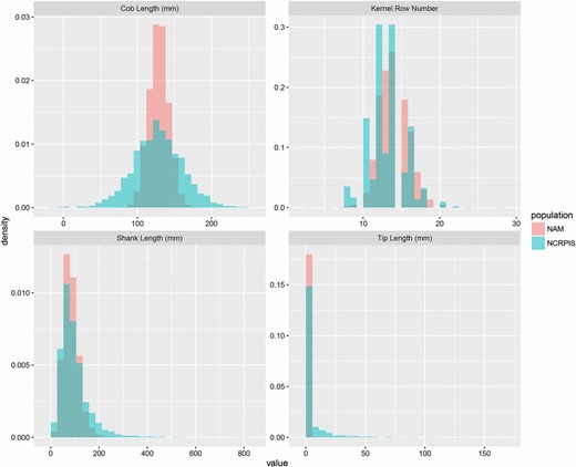
Distribution of shank length, cob length, kernel row number, and masculinized ear tip length in the NCRPIS panel and the NAM population.
Summary statistics and heritability estimates () for three domestication-related traits: shank length (SL), cob length (CL), and kernel row number (KRN) in the maize NCRPIS diversity and NAM panels
| Statistic | NCRPIS panel | NAM | ||||
|---|---|---|---|---|---|---|
| SLa (mm) | CL (mm) | KRN | SLb (mm) | CL (mm) | KRN | |
| Nc | 5,002 | 3,381 | 4,776 | 6,903 | 32,031 | 6,266 |
| Ngd | 2,387 | 2,287 | 2,339 | 2,875 | 4,359 | 2,724 |
| Mean | 95 | 141 | 14 | 87 | 129 | 14 |
| Min | 10 | 10 | 6 | 10 | 79 | 4 |
| Max | 800 | 270 | 28 | 354 | 180 | 24 |
| 0.53 | 0.40 | 0.46 | 0.42 | 0.70 | 0.38 | |
| SE()e | 0.049 | 0.045 | 0.049 | 0.031 | 0.021 | 0.031 |
SE() of SL estimated using log-transformed data.
SE() of SL estimated using square-root-transformed data.
Total number of plots measured.
Total number of inbred lines measured.
Approximate standard error of heritability estimate.
| Statistic | NCRPIS panel | NAM | ||||
|---|---|---|---|---|---|---|
| SLa (mm) | CL (mm) | KRN | SLb (mm) | CL (mm) | KRN | |
| Nc | 5,002 | 3,381 | 4,776 | 6,903 | 32,031 | 6,266 |
| Ngd | 2,387 | 2,287 | 2,339 | 2,875 | 4,359 | 2,724 |
| Mean | 95 | 141 | 14 | 87 | 129 | 14 |
| Min | 10 | 10 | 6 | 10 | 79 | 4 |
| Max | 800 | 270 | 28 | 354 | 180 | 24 |
| 0.53 | 0.40 | 0.46 | 0.42 | 0.70 | 0.38 | |
| SE()e | 0.049 | 0.045 | 0.049 | 0.031 | 0.021 | 0.031 |
SE() of SL estimated using log-transformed data.
SE() of SL estimated using square-root-transformed data.
Total number of plots measured.
Total number of inbred lines measured.
Approximate standard error of heritability estimate.
QTL and association mapping
In the NAM population, we identified 10 QTL for shank length (each associated with 1.8–2.8% of the trait variation), 8 QTL for kernel row number (associated with 1.8–7.3% variation), and 20 QTL for cob length (associated with 0.8–2.9% variation; Table S1). No QTL were detected for masculinized ear tips; power of QTL detection for this trait was limited because its segregation was restricted to one biparental family. QTL analysis within this one family did not identify any QTL passing a genome-wide permutation-based threshold of α = 0.05. Comparisons between the positions of domestication-related trait QTL mapped in NAM and previously identified domestication QTL mapped in crosses between maize and teosinte revealed little correspondence between the two sets of QTL (Figure S1, Figure S2, and Figure S3). Genome-wide association scans conducted in the NCRPIS diversity panel identified 0, 5, and 10 SNPs associated with cob length, shank length, and kernel row number, respectively, at FDR < 0.05 (Table S2). In general, there was limited overlap between known domestication QTL and SNPs associated with domestication-related traits in either panel (Figure S1, Figure S2, and Figure S3); however, a few notable correspondences were observed. A SNP 270,000 bp upstream of fea2 was strongly associated with the kernel row number trait; however, the one SNP inside of the fea2 coding region was not significant. Several associations identified for shank length (SL) in NAM are in the vicinity of tb1, but ∼2 million bp downstream of the gene (Table S3). By contrast, the known upstream enhancer of tb1 is ∼59–69 kbp from the coding start site (Clark et al. 2006; Studer et al. 2011).
Testing concordance between loci associated with domestication traits within maize and loci that distinguish maize from teosinte
For each set of trait QTL and SNP associations, we compared the mean r2 of associations inside vs. outside genomic regions previously identified as related to domestication. Domestication QTL were mapped in a maize-by-teosinte cross population by Briggs et al. (2007) (Table S4) and domestication selection sweep regions were identified from population genetics analyses (Hufford et al. 2012). In addition, we compared mean r2 of associations for SNPs inside or outside regions defined as postdomestication “improvement” selection sweeps from population genetics analyses (Hufford et al. 2012). To remove the potentially confounding effect of variability in gene density among regions tested, we tested within regions defined using both annotation for involvement in domestication or improvement and annotation for coding or noncoding regions.
For the NCRPIS diversity panel, mean marker r2 values were ∼0.0009, and the largest difference between groups was only 0.000032 (Table 2). This maximum difference was observed between coding variants inside and outside of domestication QTL for kernel row number (KRN), and the SNPs outside of the domestication QTL were associated with more variation (Table 2). In fact, the only significant differences in mean marker r2 for SNPs classified according to domestication QTL were observed when SNPs outside of QTL were associated with greater mean r2 values than SNPs within the QTL (Table 2). Further, there was no consistent evidence that SNPs inside domestication or improvement sweeps were associated with more variation than SNPs outside of these regions, although noncoding SNPs within sweep regions had significantly higher mean r2 values for shank length than noncoding SNPs outside those regions (Table 2).
Mean SNP association r2 and number of markers (Nm) inside and outside hypothesis-defined testing regions in the NCRPIS panel
| Shank length | Cob length | Kernel row number | |||||
|---|---|---|---|---|---|---|---|
| r2: | Nm: | r2: | Nm: | r2: | Nm: | ||
| Hypothesis or background | Coding or noncoding | ×10−4 | N × 103 | ×10−4 | N × 103 | ×10−4 | N × 103 |
| Domestication QTL | |||||||
| Hypothesis | Coding | 9.27 | 21.5 | 9.18 | 27.2 | 9.20 | 17.8 |
| Background | Coding | 9.19 | 226.4 | 9.40 | 220.7 | 9.52 | 230.2 |
| Difference | Coding | 0.08 | −0.22** | −0.32** | |||
| Hypothesis | Noncoding | 9.09 | 15.4 | 9.16 | 19.6 | 9.43 | 13.6 |
| Background | Noncoding | 9.29 | 141.9 | 9.38 | 137.7 | 9.42 | 143.7 |
| Difference | Noncoding | −0.20** | −0.22 | 0.01 | |||
| Domestication sweep | |||||||
| Hypothesis | Coding | 9.30 | 15.0 | 9.39 | 15.0 | 9.45 | 15.0 |
| Background | Coding | 9.20 | 232.9 | 9.37 | 232.9 | 9.50 | 232.9 |
| Difference | Coding | 0.10 | 0.02 | −0.05 | |||
| Hypothesis | Noncoding | 9.52 | 10.4 | 9.31 | 10.4 | 9.52 | 10.4 |
| Background | Noncoding | 9.25 | 146.9 | 9.35 | 146.9 | 9.41 | 146.9 |
| Difference | Noncoding | 0.27** | −0.04** | 0.11 | |||
| Improvement sweep | |||||||
| Hypothesis | Coding | 9.22 | 11.9 | 9.50 | 11.9 | 9.60 | 11.9 |
| Background | Coding | 9.20 | 236.0 | 9.37 | 236.0 | 9.49 | 236.0 |
| Difference | Coding | 0.02 | 0.13 | 0.11 | |||
| Hypothesis | Noncoding | 9.56 | 9.0 | 9.53 | 9.0 | 9.20 | 9.0 |
| Background | Noncoding | 9.25 | 148.4 | 9.34 | 148.4 | 9.43 | 148.4 |
| Difference | Noncoding | 0.31** | 0.19 | −0.23* | |||
Significantly different at * P = 0.05 and ** P = 0.01, respectively.
| Shank length | Cob length | Kernel row number | |||||
|---|---|---|---|---|---|---|---|
| r2: | Nm: | r2: | Nm: | r2: | Nm: | ||
| Hypothesis or background | Coding or noncoding | ×10−4 | N × 103 | ×10−4 | N × 103 | ×10−4 | N × 103 |
| Domestication QTL | |||||||
| Hypothesis | Coding | 9.27 | 21.5 | 9.18 | 27.2 | 9.20 | 17.8 |
| Background | Coding | 9.19 | 226.4 | 9.40 | 220.7 | 9.52 | 230.2 |
| Difference | Coding | 0.08 | −0.22** | −0.32** | |||
| Hypothesis | Noncoding | 9.09 | 15.4 | 9.16 | 19.6 | 9.43 | 13.6 |
| Background | Noncoding | 9.29 | 141.9 | 9.38 | 137.7 | 9.42 | 143.7 |
| Difference | Noncoding | −0.20** | −0.22 | 0.01 | |||
| Domestication sweep | |||||||
| Hypothesis | Coding | 9.30 | 15.0 | 9.39 | 15.0 | 9.45 | 15.0 |
| Background | Coding | 9.20 | 232.9 | 9.37 | 232.9 | 9.50 | 232.9 |
| Difference | Coding | 0.10 | 0.02 | −0.05 | |||
| Hypothesis | Noncoding | 9.52 | 10.4 | 9.31 | 10.4 | 9.52 | 10.4 |
| Background | Noncoding | 9.25 | 146.9 | 9.35 | 146.9 | 9.41 | 146.9 |
| Difference | Noncoding | 0.27** | −0.04** | 0.11 | |||
| Improvement sweep | |||||||
| Hypothesis | Coding | 9.22 | 11.9 | 9.50 | 11.9 | 9.60 | 11.9 |
| Background | Coding | 9.20 | 236.0 | 9.37 | 236.0 | 9.49 | 236.0 |
| Difference | Coding | 0.02 | 0.13 | 0.11 | |||
| Hypothesis | Noncoding | 9.56 | 9.0 | 9.53 | 9.0 | 9.20 | 9.0 |
| Background | Noncoding | 9.25 | 148.4 | 9.34 | 148.4 | 9.43 | 148.4 |
| Difference | Noncoding | 0.31** | 0.19 | −0.23* | |||
Significantly different at * P = 0.05 and ** P = 0.01, respectively.
For the NAM population, the mean SNP r2 values were significantly different for each comparison of hypothesis region and grouping based on coding regions (Table 3). The largest differences between categories were observed between SNPs inside and outside of domestication QTL for KRN. Domestication QTL SNPs were associated with more variation only for KRN, whereas domestication QTL SNPs had smaller mean r2 values for SL and cob length (CL) (Table 3). SNP variances were larger inside than outside of hypothesis regions most consistently for domestication sweep regions, but even within this group, SNPs in noncoding domestication sweep regions had lower mean r2 values associated with CL than SNPs in noncoding regions outside of domestication sweep regions (Table 3).
Mean SNP association r2 and number of markers (Nm) inside and outside hypothesis-defined testing regions in the NAM panel
| Shank length | Cob length | Kernel row number | |||||
|---|---|---|---|---|---|---|---|
| r2: | Nm: | r2: | Nm | r2: | Nm: | ||
| Hypothesis or background | Coding or noncoding | ×10−4 | N × 105 | ×10−4 | N × 105 | ×10−4 | N × 105 |
| Domestication QTL | |||||||
| Hypothesis | Coding | 9.97 | 2.1 | 17.2 | 2.9 | 29.7 | 2.1 |
| Background | Coding | 14.3 | 20.6 | 20.8 | 20.3 | 20.0 | 20.6 |
| Difference | Coding | −4.3** | −3.6** | 9.7** | |||
| Hypothesis | Noncoding | 10.1 | 32.9 | 18.5 | 42.5 | 25.6 | 28.4 |
| Background | Noncoding | 14.9 | 201.6 | 25.8 | 196.9 | 22.5 | 206.0 |
| Difference | Noncoding | −4.8** | −7.3* | 3.1** | |||
| Domestication sweep | |||||||
| Hypothesis | Coding | 15.3 | 1.2 | 20.7 | 1.2 | 29.6 | 1.2 |
| Background | Coding | 13.8 | 21.5 | 20.4 | 21.5 | 20.0 | 21.5 |
| Difference | Coding | 1.5** | 0.3** | 9.6** | |||
| Hypothesis | Noncoding | 16.1 | 15.5 | 21.1 | 15.5 | 31.4 | 15.5 |
| Background | Noncoding | 14.2 | 219.1 | 25.0 | 219.1 | 22.2 | 219.1 |
| Difference | Noncoding | 1.9** | −3.9** | 9.2** | |||
| Improvement sweep | |||||||
| Hypothesis | Coding | 12.8 | 1.4 | 25.2 | 1.4 | 17.8 | 1.4 |
| Background | Coding | 14.0 | 21.6 | 20.2 | 21.6 | 20.8 | 21.6 |
| Difference | Coding | −1.2** | 5** | −3** | |||
| Hypothesis | Noncoding | 13.9 | 10.7 | 31.3 | 10.7 | 21.2 | 10.7 |
| Background | Noncoding | 14.3 | 223.7 | 24.4 | 223.7 | 23.0 | 223.7 |
| Difference | Noncoding | −0.4** | 6.9** | −1.8** | |||
Significantly different at * P = 0.05 and ** P = 0.01, respectively.
| Shank length | Cob length | Kernel row number | |||||
|---|---|---|---|---|---|---|---|
| r2: | Nm: | r2: | Nm | r2: | Nm: | ||
| Hypothesis or background | Coding or noncoding | ×10−4 | N × 105 | ×10−4 | N × 105 | ×10−4 | N × 105 |
| Domestication QTL | |||||||
| Hypothesis | Coding | 9.97 | 2.1 | 17.2 | 2.9 | 29.7 | 2.1 |
| Background | Coding | 14.3 | 20.6 | 20.8 | 20.3 | 20.0 | 20.6 |
| Difference | Coding | −4.3** | −3.6** | 9.7** | |||
| Hypothesis | Noncoding | 10.1 | 32.9 | 18.5 | 42.5 | 25.6 | 28.4 |
| Background | Noncoding | 14.9 | 201.6 | 25.8 | 196.9 | 22.5 | 206.0 |
| Difference | Noncoding | −4.8** | −7.3* | 3.1** | |||
| Domestication sweep | |||||||
| Hypothesis | Coding | 15.3 | 1.2 | 20.7 | 1.2 | 29.6 | 1.2 |
| Background | Coding | 13.8 | 21.5 | 20.4 | 21.5 | 20.0 | 21.5 |
| Difference | Coding | 1.5** | 0.3** | 9.6** | |||
| Hypothesis | Noncoding | 16.1 | 15.5 | 21.1 | 15.5 | 31.4 | 15.5 |
| Background | Noncoding | 14.2 | 219.1 | 25.0 | 219.1 | 22.2 | 219.1 |
| Difference | Noncoding | 1.9** | −3.9** | 9.2** | |||
| Improvement sweep | |||||||
| Hypothesis | Coding | 12.8 | 1.4 | 25.2 | 1.4 | 17.8 | 1.4 |
| Background | Coding | 14.0 | 21.6 | 20.2 | 21.6 | 20.8 | 21.6 |
| Difference | Coding | −1.2** | 5** | −3** | |||
| Hypothesis | Noncoding | 13.9 | 10.7 | 31.3 | 10.7 | 21.2 | 10.7 |
| Background | Noncoding | 14.3 | 223.7 | 24.4 | 223.7 | 23.0 | 223.7 |
| Difference | Noncoding | −0.4** | 6.9** | −1.8** | |||
Significantly different at * P = 0.05 and ** P = 0.01, respectively.
Association of haplotypes at known domestication genes
A number of domestication QTL have been resolved to individual genes by a combination of high-resolution genetic mapping, mutant analysis, and gene expression studies (Table 4). We identified SNPs within and nearby these genes and defined haplotypes at each domestication gene based on multiple SNP genotypes. Haplotype tests in the NCRPIS panel indicate that haplotypes containing grassy tillers 1 (gt1) were significantly associated with shank length (1.6% of variation, P < 0.05; Table 4). Haplotype additive effects on shank length ranged from +32 mm to −26 mm for gt1 (Table S5), and the inbred lines with haplotype effects that cause the largest increase in shank length represent a set of tropical and exotic germplasm distinct from the major temperate maize breeding pool (CML254, CML270, CML388, CML389, CML419, GE440, NC264, SC276Q2, SC277, SC76, TZEEI17, TZEEI20, and TZEI5). Zea apetala homolog1 (zap1) showed a significant association with cob length (5.9% of variation, P < 0.01; Table 4 and Table S6). No other candidate gene haplotypes had significant effects on trait variation.
Tests of associations between haplotypes of known domestication genes and domestication-related traits in the NCRPIS panel
| Gene name | Chr | Starta | End | Extended testing region?b | Extended start | Extended end | No. of SNPs in gene | No. of SNPs in testing region | No. of haplotypes tested for association | Proportion of variance explained (%)c | ||
|---|---|---|---|---|---|---|---|---|---|---|---|---|
| SL | CL | KRN | ||||||||||
| tb1 | 1 | 265,745,979 | 265,747,712 | Yes | 265,746,572 | 265,751,840 | 5 | 12 | 15 | NS | NS | — |
| tb1-enhancer | 1 | 265,676,479 | 265,687,279 | No | — | — | 9 | 9 | 6 | NS | NS | — |
| gt1 | 1 | 23,241,091 | 23,244,476 | Yes | 23,236,091 | 23,249,476 | 3 | 13 | 48 | 1.6* | NS | — |
| zagl1 | 1 | 4,862,047 | 4,877,625 | Yes | 4,862,244 | 4,862,765 | 5 | 5 | 6 | — | NS | — |
| zap1 | 2 | 235,845,160 | 235,853,770 | No | — | — | 21 | 21 | 45 | — | 5.9** | — |
| te1 | 3 | 165,174,146 | 165,178,071 | No | — | — | 8 | 8 | 17 | — | NS | — |
| fea2 | 4 | 133,662,510 | 133,664,998 | Yes | 133,662,368 | 133,664,252 | 2 | 2 | 6 | — | — | NS |
Chr, chromosome. NS, not significant. Significant at * P < 0.05 and ** P < 0.01, respectively.
Coding sequence start position (AGPv2).
If the region is extended, the testing region is 5 kbp extended on the left and right sides of the original position. Sometimes SNPs do not fully spread in the whole testing region, so the extended region is the actual region for testing.
Proportion of variance explained is calculated as
| Gene name | Chr | Starta | End | Extended testing region?b | Extended start | Extended end | No. of SNPs in gene | No. of SNPs in testing region | No. of haplotypes tested for association | Proportion of variance explained (%)c | ||
|---|---|---|---|---|---|---|---|---|---|---|---|---|
| SL | CL | KRN | ||||||||||
| tb1 | 1 | 265,745,979 | 265,747,712 | Yes | 265,746,572 | 265,751,840 | 5 | 12 | 15 | NS | NS | — |
| tb1-enhancer | 1 | 265,676,479 | 265,687,279 | No | — | — | 9 | 9 | 6 | NS | NS | — |
| gt1 | 1 | 23,241,091 | 23,244,476 | Yes | 23,236,091 | 23,249,476 | 3 | 13 | 48 | 1.6* | NS | — |
| zagl1 | 1 | 4,862,047 | 4,877,625 | Yes | 4,862,244 | 4,862,765 | 5 | 5 | 6 | — | NS | — |
| zap1 | 2 | 235,845,160 | 235,853,770 | No | — | — | 21 | 21 | 45 | — | 5.9** | — |
| te1 | 3 | 165,174,146 | 165,178,071 | No | — | — | 8 | 8 | 17 | — | NS | — |
| fea2 | 4 | 133,662,510 | 133,664,998 | Yes | 133,662,368 | 133,664,252 | 2 | 2 | 6 | — | — | NS |
Chr, chromosome. NS, not significant. Significant at * P < 0.05 and ** P < 0.01, respectively.
Coding sequence start position (AGPv2).
If the region is extended, the testing region is 5 kbp extended on the left and right sides of the original position. Sometimes SNPs do not fully spread in the whole testing region, so the extended region is the actual region for testing.
Proportion of variance explained is calculated as
Variance component testing
To estimate the proportion of trait genotypic variance associated with additive polygenic vs. other genetic effects (such as large-effect loci and nonadditive variance) in the NCRPIS panel, we simultaneously modeled genotypic effects with variance–covariance relationships proportional to the realized additive relationship matrix and genotypic effects with no pairwise relationships to capture genetic effects unique to each line. Among traits, 92–100% of genotypic variance was accounted for by polygenic additive background effects, with the remainder of variance attributable to a combination of nonadditive effects and large-effect loci (Table S7).
To partition total trait variance into components associated with domestication QTL, domestication sweep regions, improvement sweep regions, and the remainder of the genome, we estimated realized additive relationship matrices using SNPs in each of these regions of the genome and estimated the associated variance components in each panel (Figure 2, Figure 3, Table S8, Table S9, and Table S10). When effects associated with all four relationship matrices were fitted simultaneously in a common mixed model, the background polygenic variance component accounted for 67–80% of the total additive genetic variance in NCRPIS (Figure 2A, Table S8, and Table S10) and 71–100% in NAM (Figure 3A, Table S9, and Table S10). The increase in total heritability explained by fitting all four categories together was only 0–1% compared to simply fitting a single relationship matrix based on all SNPs together across all traits and panels (Figure 2A, Figure 3A, Table S8, and Table S9).
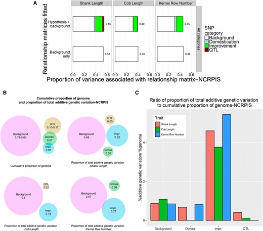
(A) The proportion of variance for shank length, cob length, and kernel row number among inbred lines of the NCRPIS panel associated with relationship matrices based on all SNPs in hypothesis-defined regions or on background SNPs. (B) Cumulative proportion of genome tagged by SNPs defining hypothesis relationship matrices and background matrices and the proportion of total additive genetic variation associated with each relationship matrix for shank length, cob length, and kernel row number among inbred lines of the NCRPIS panel. (C) Ratio of proportion of total additive genetic variation to cumulative proportion of the genome tagged by SNPs defining hypothesis and background relationship matrices for shank length, cob length, and kernel row number among inbred lines of the NCRPIS panel.
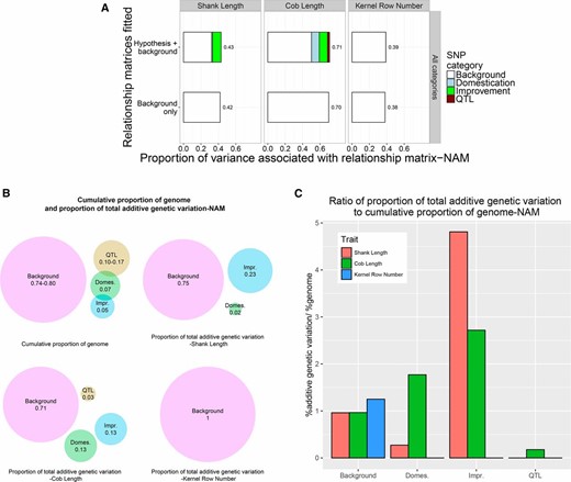
(A) The proportion of variance for shank length, cob length, and kernel row number among inbred lines of the NAM panel associated with relationship matrices based on all SNPs in hypothesis-defined regions or based on background SNPs. (B) Cumulative proportion of the genome tagged by SNPs defining hypothesis relationship matrices and background matrices and the proportion of total additive genetic variation associated with each relationship matrix for shank length, cob length, and kernel row number among inbred lines of the NAM panel. (C) Ratio of proportion of total additive genetic variation to cumulative proportion of the genome tagged by SNPs defining hypothesis and background relationship matrices for shank length, cob length, and kernel row number among inbred lines of the NAM panel.
The relationship matrices were estimated using widely different numbers of markers, which is expected to affect the proportion of variance associated with each matrix under the null hypothesis of equal contributions to the total genetic variance. Therefore, we compared the proportion of additive variance accounted for by each matrix to the proportion of the genome represented by the hypothesis region. The proportion of additive variance associated with QTL-defined and domestication sweep-related hypothesis matrices was smaller than the proportion of genome represented by the SNPs defining those matrices (except for cob length in the NAM population; Figure 2, Figure 3, and Table S10). In contrast, the proportion of total additive variance associated with the improvement sweep-defined relationship matrix was two to five times greater than the proportion of the genome represented by the improvement sweeps (except for kernel row number variance, which was completely associated with the genomic background; Figure 2, Figure 3, and Table S10).
An alternative approach to account for differences in the proportion of the genome represented in each matrix was to fit each hypothesis-based relationship matrix along with a matched background relationship matrix based on an equally sized sample of background SNPs with the same proportion of coding and noncoding variants to estimate variance components. For each combination of hypothesis region, trait, and inbred line panel, we sampled background SNPs and fitted the mixed model 20 times to estimate the variability in variance components estimates across samples. Background polygenic effects were consistently associated with more variance than the domestication QTL, domestication sweep, or improvement sweep regions when fitting relationship matrices with matching numbers and genic composition of SNPs (Figure S4, Figure S5, Table S8, and Table S9). Among the hypothesis-defined regions, the improvement sweep regions consistently explained the largest proportion of variation, ranging from 8% to 48% of the total heritable variance when fitted with a matched background polygenic effect relationship matrix.
Discussion
Heritability and polygenic variation
Heritabilities of the three traits were relatively low to moderate, in part because the large numbers of lines tested precluded evaluating larger numbers of replicates of the experiment. The polygenic relationship matrix was associated with 40–53% of total phenotypic variation in the NCRPIS panel (Table 1). By comparison, the largest amount of variation associated with an individual SNP was estimated to be ∼3% (Table S2) and few SNPs passed stringent thresholds for association tests.
Haplotypes at the candidate gene zap1 were associated with 6% of cob length variation, suggesting that complex variation in a genomic region occasionally may account for more variation than can be associated with a single SNP, but this was the exception to the general trend of no obvious haplotype effects. Variants in zap1 were associated with ear length in teosinte (Weber et al. 2008); our results suggest some functional variation at this locus passed through the domestication bottleneck and remains in maize or new functional variants have arisen within maize. Haplotypes at candidate gene gt1 were also associated with a small amount of shank length variation in maize. Although this locus was not detected as affecting lateral branch (shank) length in maize–teosinte crosses (Briggs et al. 2007), Wills et al. (2013) identified gt1 as conferring the major difference in the number of ears produce by maize and teosinte and observed that haplotypic variation at this locus suggests only a partial sweep due to selection under domestication. Some of the teosinte-type variation at this locus may even have a favorable effect in maize by increasing the number of ears by a small amount, and it is possible that these same variants have small effects on shank length.
The tb1 gene and its linked enhancer played a key role in changing the morphology of maize, including reducing the length of lateral branches, during the domestication process (Studer et al. 2011; Tsiantis 2011). Thus, tb1 is an obvious candidate for explaining the variation among shank (lateral branch) lengths in maize. However, we observed no QTL or SNP association in NAM around tb1. We also did not identify an association for shank length near the gene in the diversity panel GWAS, and SNPs inside of the tb1 coding region and its enhancer were not significant. Direct testing of haplotypes defined by SNPs surrounding tb1 (encompassing a 5268-bp region) and encompassing the tb1 enhancer region suggested that these haplotypes are not significantly associated with shank length for the NCRPIS panel.
Although we identified a few individual SNPs and haplotypes associated with significant amounts of variation for domestication traits in maize, their effects were small. Power of association tests is influenced by sample size, allele frequency, effect size, and marker density; therefore, it is possible that some rare alleles of large effect were not detected in the GWAS scans, resulting in “missing heritability” (Manolio et al. 2009). Many SNPs are rare in the NCRPIS panel (Romay et al. 2013) and their effects are difficult to estimate accurately. Since the NAM population is derived from 25 founders crossed to a common reference parent, the minimum allele frequency expected is ∼2%, or 100 lines, which is sufficiently large to detect large-effect alleles. However, our evaluations of two of the domestication traits were based on smaller subsets of NAM, so power of detection of variants private to individual families is smaller for those traits. Interactions between causal variants at different loci (epistasis) and with environments will also make their detection more difficult (Manolio et al. 2009). Nevertheless, the lack of strong effects associated with any individual SNPs and the relatively large proportion of variation associated with the genomic background indicate that the genetic architecture of variation for domestication traits within maize is distinct from the genetic control of differences between maize and teosinte, which is dominated by a relatively few large-effect loci.
We found no evidence that QTL or SNP associations for these traits were more likely to be near domestication QTL or that markers in domestication QTL explained more trait variation than markers outside of these regions (Figure 2, Figure 3, Table 2, and Table 3). No consistent pattern of increased SNP effects was observed for SNPs inside domestication or improvement sweep regions (Table 2 and Table 3). The comparison of average SNP effects averaged over all SNPs in a group has limitations; many of these effect estimates are expected to be poor, and the mean value estimated is expected to be an upwardly biased estimate of the true mean effect size of individual SNPs. However, by averaging over many thousands of loci within each class, we expect the biases to cancel out when comparing mean effect sizes of different classes.
Partitioning of the genetic variance into components due to specific hypothesis-based regions is likely a more reliable method for comparing the influence of different genomic regions that are highly polygenic. Using this approach, we observed that improvement sweep regions showed a consistently higher proportion of the total heritable variance than other hypothesis-defined regions and often substantially more than the proportion of the genome represented by SNPs defining the improvement sweep relationship matrix (Figure 2, Figure 3, Table S8, Table S9, and Table S10). When we fitted specific hypothesis-based relationship matrices along with background matrices sampled with matching SNP numbers and proportion of coding SNPs, the variance associated with hypothesis-based relationship matrices was always lower than the matching background (Figure S4 and Figure S5). However, although we took care to control for the sample size and gene density of the SNPs used to compute the hypothesis and background relationship matrices, we expect that the markers used for the hypothesis matrix have higher linkage disequilibrium and relatively less explanatory power than equally sized samples of SNPs from the rest of the genome because they were sampled from restricted genomic blocks. The higher levels of linkage disequilibrium expected among the improvement sweep SNPs would downwardly bias the proportion of total additive variance they can explain relative to an equally sized random sample of SNPs from the rest of the genome. Therefore, these results are congruent with enrichment of improvement sweep-related regions of the maize genome for functional variants affecting domestication-related traits, although the effects of individual variants appear to be quite small and the precise magnitude of the enrichment remains difficult to assess.
The generally reduced contribution of domestication QTL regions, and to a lesser extent the domestication sweep regions, to domestication-related traits variation in maize is likely a direct result of selection purging variants that favor the teosinte morphology in these regions. Theory and analysis of response to long-term artificial selection in a number of plant and animal species indicate that initial generations of selection response are due to standing variation in the initial population, but that genetic variation in later generations is usually mostly due to the effects of new mutations (Keightley 2004; Walsh 2004). Thus, mutation is expected to be an important generator of genetic variation over the several thousand generations of selection and evolution of distinct maize types from a common ancestral population following the domestication bottleneck. Our results suggest that if new mutations that occurred after domestication are responsible for some of the observed genetic variation in domestication traits, they occur at genes not involved in domestication.
The increased contribution of improvement sweep regions to variation in these traits may be due to divergent selection for functional alleles in these regions. Although modern inbreds are significantly differentiated from landraces in these regions, the level of differentiation is lower than the mean differentiation between landraces and teosinte in the domestication sweep regions (Hufford et al. 2012). Thus, more sequence variation exists among inbreds in improvement sweep regions than in domestication sweep regions. However, less variation among inbreds exists in both domestication and improvement sweep regions than in the rest of the genome. This suggests that functional variants for domestication traits in improvement sweep regions may be targets of selection, but divergent selection maintains some variation for such variants. For example, some maize varieties have small kernel row numbers (because this is associated with larger seed size); others with small cob lengths are maintained because they have favored kernel types. Historical selection may have favored more kernel rows and longer cobs in general, but diverse inbred lines sampled from different regions may include contributions from populations selected in the opposite direction, resulting in an overall signal of selection near variants that affect these traits at the same time as these variants contribute disproportionately to the observed trait variation.
Acknowledgments
We thank Jeff Glaubitz for help selecting SNPs from the HapMap 3 database for relationship matrix estimation. S.X. was supported by National Institutes of Environmental Health Sciences training grant T32 ES007329 to the North Carolina State University Bioinformatics Research Center and National Science Foundation (NSF) award IOS-1127076; J.B.H. was supported by NSF awards IOS-1127076 and IOS-1238014 and by the U.S. Department of Agriculture, Agricultural Research Service.
Footnotes
Communicating editor: A. H. Paterson
Supplemental material is available online at www.genetics.org/lookup/suppl/doi:10.1534/genetics.116.191106/-/DC1.
Literature Cited
Bass, A. J., A. Dabney, and D. Robinson, 2015 Qvalue: Q-Value Estimation for False Discovery Rate Control. R Package version 2.2.2. Available at: http://github.com/jdstorey/qvalue.
R Core Team, 2016 R: A language and environment for statistical computing. R Foundation for Statistical Computing, Vienna, Austria. Available at: https://www.R-project.org/.
