


Abstract
The genetic structure of human populations is often characterized by aggregating measures of ancestry across the autosomal chromosomes. While it may be reasonable to assume that population structure patterns are similar genome-wide in relatively homogeneous populations, this assumption may not be appropriate for admixed populations, such as Hispanics and African-Americans, with recent ancestry from two or more continents. Recent studies have suggested that systematic ancestry differences can arise at genomic locations in admixed populations as a result of selection and nonrandom mating. Here, we propose a method, which we refer to as the chromosomal ancestry differences (CAnD) test, for detecting heterogeneity in population structure across the genome. CAnD can incorporate either local or chromosome-wide ancestry inferred from SNP genotype data to identify chromosomes harboring genomic regions with ancestry contributions that are significantly different than expected. In simulation studies with real genotype data from phase III of the HapMap Project, we demonstrate the validity and power of CAnD. We apply CAnD to the HapMap Mexican-American (MXL) and African-American (ASW) population samples; in this analysis the software RFMix is used to infer local ancestry at genomic regions, assuming admixing from Europeans, West Africans, and Native Americans. The CAnD test provides strong evidence of heterogeneity in population structure across the genome in the MXL sample (), which is largely driven by elevated Native American ancestry and deficit of European ancestry on the X chromosomes. Among the ASW, all chromosomes are largely African derived and no heterogeneity in population structure is detected in this sample.
TECHNOLOGICAL advancements in high-throughput genotyping and sequencing technologies have allowed for unprecedented insight into the genetic structure of human populations. Population structure studies have largely focused on populations of European descent, and ancestry differences among European populations have been well studied and characterized (Novembre et al. 2008; Nelis et al. 2009). Recent studies have also investigated the genetic structure of more diverse populations, including recently admixed populations, such as African-Americans (Zakharia et al. 2009; Bryc et al. 2010a) and Hispanics (Manichaikul et al. 2012; Conomos et al. 2016), who have experienced admixing within the past few hundred years from two or more ancestral populations from different continents.
Both continental and fine-scale genetic structures of human populations have largely been characterized by aggregating measures of ancestry across the autosomal chromosomes. While it may be reasonable to assume that population structure patterns across the genome are similar for populations with ancestry derived from a single continent, such as populations of European descent, this may not be a reasonable assumption for admixed populations who have recent ancestry from multiple continents. For example, a previous genetic analysis of Puerto Rican samples identified multiple chromosomes harboring large chromosomal regions with systematic ancestry differences, compared to what would be expected based on genome-wide ancestry and thus providing strong evidence of recent selection in this admixed population (Tang et al. 2007). Sex-specific patterns of nonrandom mating at the time of or since admixture can also result in systematic differences in ancestry at genomic loci as well as across entire chromosomes, such as the X and Y chromosomes, in admixed populations. For example, a recent study compared the average inferred ancestry on the autosomes to the X chromosome in a large sample of Hispanics and African-Americans (Bryc et al. 2015), and highly significant differences were detected. Increased Native American and African ancestry was identified on the X chromosome in the Hispanic and African-American samples, respectively, with a deficit of European ancestry compared to the autosomes.
Previous methods (Tang et al. 2007; Jin et al. 2012; Bhatia et al. 2014) have been proposed for detecting signals of selection in admixed populations by identifying genomic regions that exhibit unusually large deviations in ancestry proportions compared to expected ancestry based on genome-wide average estimates. For assessing significance, however, these methods require strong assumptions about the evolution of the admixed population of interest, which will generally be partially or completely unknown, including (1) the relative contribution from each of the ancestral populations to the gene pool at the time of the admixture events, (2) the number of generations since the admixture events, (3) an assumed effective population size, and (4) random mating. Significance is then assessed either analytically or through simulation studies based on these evolutionary assumptions. Misspecification of these assumptions, however, can result in false positives due to an assumed null distribution that is incorrect, where chromosomal regions that appear to have large ancestry differences are actually not significantly different from what would be expected when sampling variation, genetic drift after admixture, and potential bias in local ancestry estimation are appropriately taken into account (Bhatia et al. 2014).
Here, we consider the problem of detecting heterogeneity in ancestry across the genome in admixed populations. We propose the chromosomal ancestry differences (CAnD) test for the identification of chromosomes that harbor genomic regions with significantly different proportional ancestry compared to the rest of the genome. CAnD can incorporate ancestry inferred at genomic regions using “local” ancestry estimation methods, such as RFMix (Maples et al. 2013) and HAPMIX (Price et al. 2009), or chromosomal-wide ancestry estimated using “global” ancestry estimation methods, such as FRAPPE (Tang et al. 2005) and ADMIXTURE (Alexander et al. 2009). To detect heterogeneity in ancestry across the genome, CAnD tests for systematic differences in genetic contributions from the underlying ancestral populations to chromosomes. The CAnD method also takes into account correlated ancestries among chromosomes within individuals, which improves power. An important feature of CAnD is that the method does not require specification of or strong assumptions about the population history of the admixed individuals for valid testing of ancestry heterogeneity among chromosomes.
We perform simulation studies using real genotype data from phase III of the HapMap Project (Altshuler et al. 2010) to evaluate and compare both the type I error and power of CAnD to an analysis of variance (ANOVA) ancestry heterogeneity test. We also apply CAnD to the HapMap Mexican-Americans from Los Angeles (MXL) and African-Americans from the Southwest U.S. (ASW) population samples, testing population structure heterogeneity across the genome. In this analysis, the RFMix software is used to infer European, Native American, and African ancestry at genomic locations across the autosomal chromosomes and the X chromosome. We also compare heterogeneity testing between the autosomes and the X chromosome in the HapMap MXL and ASW with CAnD to a previously used heterogeneity test (Bryc et al. 2015) based on a two-sample t statistic that does not account for ancestry correlations among the autosomes and the X chromosomes in an admixed individual.
Methods
Chromosome-wide and genome-wide ancestry measures
Let n be the number of unrelated individuals sampled from an admixed population derived from K ancestral subpopulations. We assume that there is variability in proportional ancestry among the sampled individuals, and for individual we define the genome-wide ancestry of i to be the average ancestry across both the autosomal and the X chromosomes. (For males, ancestry on the Y chromosome could also be included when calculating genome-wide ancestry if Y chromosomal ancestry information is available.) We denote the genome-wide ancestry vector for individual i to be where is the proportion of ancestry from subpopulation k for individual i, for all k, and
Let be the set of autosomal and X chromosomes, i.e., and denote the genetic ancestry of individual i for a particular chromosome to be For each chromosome c, let be the set of all chromosomes excluding c; i.e., and Define to be the mean subpopulation k ancestry for individual i across all chromosomes except for chromosome c; i.e., chromosome c is not included in the average ancestry calculation. Note that for individual i, corresponds to the average autosomal ancestry for subpopulation k. We define to be the difference in ancestry from subpopulation k for individual i between a given chromosome c and the average ancestry of all other chromosomes.
The CAnD test
Note that CAnD is a very flexible approach and one can test for ancestry differences between two chromosomes by considering a subset containing only two elements. One can also test for differences in ancestry between a single chromosome c and the pooled ancestry of all of the other chromosomes in with CAnD by letting in Equation 2 and where is set equal to the multiplicative inverse of the estimated scalar variance of For example, to test for ancestry differences between the autosomes and the X chromosome, one can let In this case, would be a univariate random variable, and under the null hypothesis of no association the test statistics would follow a distribution with 1 d.f.
The proposed CAnD test can be viewed as an application of a more general approach for assessing differences in mean values among correlated groups. For example, previous methods using this general approach have been developed for valid genetic association testing between a phenotype and genetic markers in correlated samples (Wei and Johnson 1985; Xu et al. 2003; Yang et al. 2010; Zhu et al. 2015), and CAnD is an adaptation of this approach for detecting heterogeneity in ancestry across the genome while accounting for correlations among chromosomes within an admixed individual.
Simulation studies
To assess type I error and power of the CAnD method, we performed simulation studies using real genotype data from the HapMap Utah residents with ancestry from northern and western Europe from the Centre d’Étude du Polymorphisme Humain collection (CEU) and Yoruba in Ibadan, Nigeria (YRI) populations. For each simulation iteration, 22 autosomal chromosomes were simulated for 50 admixed individuals that were derived from 118 CEU and 118 YRI haplotypes (Altshuler et al. 2010), where chromosomal haplotypes consisted of markers obtained from a subset of linkage disequilibrium (LD) pruned SNPs, using an threshold of 0.2 across each autosomal chromosome. Chromosome 1 yielded the largest set of LD-pruned SNPs, with 7686 SNPs, and the smallest was chromosome 21 with 1511 SNPs. The total set of LD-pruned SNPs was 93,618.
Each simulated admixed individual has admixture vectors for chromosomes 1–22 of the form respectively, where and are the population 1 and population 2 ancestry proportions for individual i on chromosome j, respectively, where and We denote CEU and YRI to be populations 1 and 2, respectively, in the simulation study. The proportional CEU ancestry on chromosome j for individual i is where is drawn from a uniform distribution on [0.05, 0.45] and is the same for all chromosomes j, and is a random ancestry effect for chromosome j that follows a distribution, where The variance of used in the simulation studies was based on the estimated average variance of European ancestry across the autosomal chromosomes within admixed individuals from the HapMap MXL sample. Under the null hypothesis, for all i.e., all chromosomes have the same mean ancestry. Under the alternative hypothesis, there is at least one such that A variety of values were considered to evaluate power as well as assess type I error at different significance levels.
A chromosome j haplotype for individual i was simulated conditional on where the haplotype is constructed to have a proportion of alleles derived from the CEU haplotypes and the remaining proportion of alleles from the YRI haplotypes. For example, if an individual i has a chromosome 1 admixture vector with a 60% European ancestry component and a 40% African ancestry component, then an admixed chromosome 1 haplotype for i is constructed to have 60% the alleles derived from the CEU haplotypes, where each CEU allele at a SNP is randomly chosen from one of the CEU haplotypes, and the remaining 40% of the alleles are similarly derived from one of the YRI haplotypes. Haplotype pairs were simulated for each of the 22 chromosomes, and there was one haplotype ancestry switch for each simulated admixed haplotype.
Chromosome-wide ancestry proportions were estimated for each individual using the FRAPPE software program (Tang et al. 2005), which implements a likelihood-based model to infer each individual’s proportional ancestry. It is important to note that using a different ancestry switching model from the one considered in this simulation study would not affect the ancestry estimates with FRAPPE since the software takes as input unphased genotypes and does not model LD between SNPs. The number of ancestral populations was set to 2 in the FRAPPE analysis, and 58 CEU and 57 YRI HapMap individuals were included as reference population samples for European and African ancestry, respectively. The CEU and YRI reference samples used in the FRAPPE analyses were different from those used to simulate the genotype data for the admixed individuals. With the resulting FRAPPE estimated chromosomal ancestries, the CAnD method was used to assess detection of heterogeneity in population structure across the 22 chromosomes.
HapMap MXL and ASW
We considered detection of heterogeneity in ancestry across the genome in unrelated HapMap MXL and ASW samples. REAP (Thornton et al. 2012) was used to infer both known and cryptic relatedness in the MXL and ASW, and a subset of 53 MXL individuals and a subset of 45 ASW individuals with kinship inferred to be less than third-degree relatives were identified to be “unrelated” and included for the ancestry heterogeneity analysis. There were 27 females and 26 males in the unrelated HapMap MXL subset and 25 females and 20 males in the unrelated HapMap ASW subset. We also performed CAnD tests stratified by sex to determine whether there was any bias in the results due to X chromosome copy number differences for males and females.
We used the RFMix software (Maples et al. 2013) to estimate local ancestry across the autosomes and the X for all HapMap MXL and ASW samples. RFMix allows for multiple ancestral subpopulations in a local ancestry analysis, and ancestral contributions from African, European, and Native American populations were assumed for both the HapMap MXL and ASW. The HapMap CEU and YRI samples were included as the reference population panels for European and African ancestry, respectively, and the Human Genome Diversity Project (HGDP) (Li et al. 2008) samples from the Americas were included as the reference population panel for Native American ancestry in the RFMix local ancestry analysis of the MXL and ASW. All samples were phased and sporadic missing genotypes were imputed using the BEAGLE v.3 software (Browning and Browning 2007). Recombination maps for each chromosome were downloaded from the HapMap website (Altshuler et al. 2010) and were converted to Human Genome Build 36. There was no phasing conducted on the X for the males in the sample since a male individual has only one X chromosome. Only SNPs that were genotyped in both the HapMap and HGDP data sets were considered in the local ancestry analysis. For local ancestry on the X chromosome, only SNPs on the non-pseudoautosomal regions, where there is no homology between the X and Y chromosomes, were considered.
We also conducted a CAnD analysis using chromosome-wide ancestry estimates from the FRAPPE software (Tang et al. 2005) and we compared the results to the aforementioned CAnD analysis that used local ancestry estimates from RFMix. For each chromosome, supervised global ancestry analyses were conducted separately for the HapMap MXL and ASW population samples with FRAPPE. The number of ancestral populations was set to three in each FRAPPE analysis, and the same reference population samples used in the RFMix local ancestry analysis were also used with FRAPPE. Since males only have one allele at each of the X chromosome SNPs, one of the alleles at an X-linked SNP was coded to be missing in the FRAPPE analysis of the X chromosome, although we found that coding male genotypes as homozygous in the FRAPPE analysis yielded nearly identical X chromosome ancestry results.
Data availability
The CAnD method is implemented in the R language and is available from Bioconductor (http://www.bioconductor.org) as part of the CAnD package.
Results
Assessment of type I error
As described in the Methods section, FRAPPE was used to estimate proportional ancestry for the simulated 22 chromosomes for each admixed individual. We evaluated the performance of FRAPPE when using unphased genotypes from 5000 SNPs on a chromosome by comparing the FRAPPE ancestry estimates to the simulated ancestry for chromosomes 1 and 2. The mean difference between the FRAPPE estimates and the simulated ancestry proportion values on chromosomes 1 and 2 was −5.2e-06 (SD = 0.018), thus indicating that FRAPPE provided accurate estimates of chromosome-wide ancestry (Supplemental Material, Figure S1) with no obvious bias.
To assess the type I error rate of CAnD, we simulated admixed chromosomes for 50 sampled individuals under the null hypothesis of no ancestry differences among the chromosomes, on average. The empirical type I error rates for the CAnD test at the 0.01, 0.005, and 0.001 significance levels calculated using 5000 simulated replicates are given in Table 1. The CAnD test is properly calibrated for all significance levels considered, with empirical type I error rates that are not significantly different from the nominal levels, as can be seen from the 95% confidence intervals given in Table 1. We also assessed type I error for an ANOVA test, and similar to CAnD, ANOVA is also properly calibrated under the null.
Empirical type I error
| α | CAnD empirical type I error (95% C.I.) |
|---|---|
| 0.01 | 0.0118 (0.009, 0.015) |
| 0.005 | 0.0053 (0.003, 0.007) |
| 0.001 | 0.0004 (0, 0.0013) |
| α | CAnD empirical type I error (95% C.I.) |
|---|---|
| 0.01 | 0.0118 (0.009, 0.015) |
| 0.005 | 0.0053 (0.003, 0.007) |
| 0.001 | 0.0004 (0, 0.0013) |
Shown is CAnD empirical type I error (95% C.I.) at significance levels 0.01, 0.005, and 0.001 based on 5000 simulated replicates. This simulation setting was conducted under the null hypothesis where the randomly drawn ancestry proportions of an admixed individual are the same for all chromosomes.
| α | CAnD empirical type I error (95% C.I.) |
|---|---|
| 0.01 | 0.0118 (0.009, 0.015) |
| 0.005 | 0.0053 (0.003, 0.007) |
| 0.001 | 0.0004 (0, 0.0013) |
| α | CAnD empirical type I error (95% C.I.) |
|---|---|
| 0.01 | 0.0118 (0.009, 0.015) |
| 0.005 | 0.0053 (0.003, 0.007) |
| 0.001 | 0.0004 (0, 0.0013) |
Shown is CAnD empirical type I error (95% C.I.) at significance levels 0.01, 0.005, and 0.001 based on 5000 simulated replicates. This simulation setting was conducted under the null hypothesis where the randomly drawn ancestry proportions of an admixed individual are the same for all chromosomes.
Power evaluation and comparison
We evaluated the power of CAnD for detecting heterogeneity in ancestry across 22 autosomal chromosomes in simulated samples with 50 admixed individuals. We also compared the power of CAnD to an ANOVA test that does not account for correlation in ancestry across chromosomes within an admixed individual. In the simulation studies, all autosomal chromosomes, except for chromosome 2, were chosen to have the same mean ancestry, on average. Chromosome 2 had a mean ancestry difference of from the other autosomal chromosomes, and we considered values of ranging from 0.005 to 0.2.
Empirical power results for CAnD and ANOVA at a significance level of are given in Figure 1. CAnD has significantly higher power than ANOVA for detecting low to moderate chromosomal ancestry differences. For example, there is essentially no power to detect a mean ancestry difference of between chromosome 2 and all other chromosomes with ANOVA, while CAnD has power that is close to 1. The substantial loss in power with ANOVA is due to the method not accounting for correlated ancestry among chromosomes in the simulation study that has considerable between-individual variation in proportional ancestry. In practice, we expect that the CAnD test will provide higher power than ANOVA for detecting ancestry differences among chromosomes in recently admixed populations, such as Hispanics, who have large variation in continental admixture (Conomos et al. 2016).
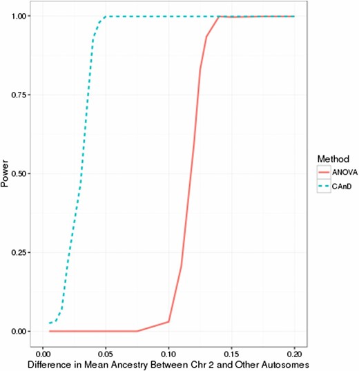
Empirical power of CAnD and ANOVA tests with simulated data. Shown is the proportion of tests rejected at a significance level of 0.01 with the CAnD and ANOVA tests for mean ancestry difference values between chromosome 2 and the other 21 autosomal chromosomes ranging from 0.005 to 0.2. For each simulated mean ancestry difference setting, the proportion of tests rejected among 500 independent simulated replicates is shown, where each replicate sample contains 50 admixed individuals.
HapMap ASW ancestry
Table 2 shows the mean and SD of the local ancestry estimates for ASW by chromosome in each of the ancestral populations, and Figure 2A shows violin plots of the local ancestry results by chromosome. The ASW are largely African derived with significantly less European ancestry. Across both the autosomes and the X chromosome, proportional Native American, on average, is quite small in the ASW relative to African and European ancestry. Interestingly, RFMix estimated 57 of the 87 ASW individuals to have no Native American ancestry on the X chromosome and 11 individuals to have no European ancestry on the X chromosome. There were 9 ASW individuals estimated to have an X chromosome that is entirely African derived. Proportional African ancestry on the autosomes ranged from 0.56 to 0.97 and ranged from 0.33 to 1 on the X. The ASW ancestry patterns on the autosomes and the X can be seen in the bar plots shown in Figure 3A, which displays the proportion of ancestry for each sampled individual.
Summary of local ancestry estimates by chromosome
| ASW | MXL | |||||
|---|---|---|---|---|---|---|
| Chr | African | European | Native American | African | European | Native American |
| X | 0.820 (0.139) | 0.163 (0.136) | 0.017 (0.047) | 0.0396 (0.0521) | 0.387 (0.245) | 0.574 (0.248) |
| Autosomal-wide | 0.783 (0.0861) | 0.202 (0.0808) | 0.0150 (0.0382) | 0.0489 (0.0182) | 0.508 (0.149) | 0.444 (0.148) |
| 1 | 0.762 (0.13) | 0.228 (0.131) | 0.00962 (0.0354) | 0.047 (0.0389) | 0.525 (0.192) | 0.428 (0.191) |
| 2 | 0.789 (0.132) | 0.201 (0.128) | 0.0106 (0.0241) | 0.0457 (0.0379) | 0.514 (0.195) | 0.440 (0.188) |
| 3 | 0.769 (0.155) | 0.221 (0.154) | 0.0102 (0.0369) | 0.0462 (0.0345) | 0.514 (0.18) | 0.439 (0.183) |
| 4 | 0.807 (0.136) | 0.177 (0.134) | 0.0164 (0.0398) | 0.0461 (0.0408) | 0.470 (0.212) | 0.484 (0.206) |
| 5 | 0.786 (0.149) | 0.199 (0.146) | 0.0148 (0.0536) | 0.0539 (0.05) | 0.528 (0.2) | 0.418 (0.188) |
| 6 | 0.774 (0.167) | 0.201 (0.15) | 0.0257 (0.0696) | 0.0555 (0.0502) | 0.500 (0.179) | 0.445 (0.177) |
| 7 | 0.804 (0.125) | 0.184 (0.117) | 0.012 (0.0539) | 0.056 (0.047) | 0.524 (0.193) | 0.420 (0.188) |
| 8 | 0.785 (0.163) | 0.201 (0.16) | 0.0141 (0.0419) | 0.0397 (0.0349) | 0.504 (0.187) | 0.456 (0.179) |
| 9 | 0.772 (0.12) | 0.210 (0.116) | 0.0175 (0.0506) | 0.0499 (0.0521) | 0.489 (0.21) | 0.462 (0.213) |
| 10 | 0.785 (0.145) | 0.205 (0.14) | 0.00997 (0.047) | 0.059 (0.066) | 0.502 (0.189) | 0.439 (0.183) |
| 11 | 0.778 (0.141) | 0.212 (0.139) | 0.00953 (0.0255) | 0.0402 (0.0422) | 0.525 (0.202) | 0.435 (0.201) |
| 12 | 0.779 (0.142) | 0.202 (0.137) | 0.0186 (0.0625) | 0.0501 (0.0488) | 0.511 (0.18) | 0.439 (0.177) |
| 13 | 0.804 (0.152) | 0.180 (0.149) | 0.0165 (0.032) | 0.0488 (0.0424) | 0.523 (0.199) | 0.428 (0.201) |
| 14 | 0.802 (0.162) | 0.183 (0.155) | 0.015 (0.0577) | 0.0559 (0.0643) | 0.470 (0.217) | 0.474 (0.219) |
| 15 | 0.817 (0.141) | 0.172 (0.138) | 0.0109 (0.0399) | 0.0382 (0.0452) | 0.528 (0.182) | 0.434 (0.179) |
| 16 | 0.778 (0.192) | 0.201 (0.183) | 0.0207 (0.0631) | 0.0456 (0.0449) | 0.498 (0.205) | 0.457 (0.209) |
| 17 | 0.772 (0.156) | 0.207 (0.145) | 0.0208 (0.079) | 0.041 (0.043) | 0.533 (0.195) | 0.426 (0.192) |
| 18 | 0.772 (0.21) | 0.210 (0.196) | 0.0184 (0.0605) | 0.0501 (0.047) | 0.537 (0.207) | 0.413 (0.198) |
| 19 | 0.780 (0.154) | 0.213 (0.155) | 0.00745 (0.0189) | 0.0654 (0.0809) | 0.506 (0.208) | 0.429 (0.202) |
| 20 | 0.801 (0.167) | 0.187 (0.152) | 0.0125 (0.0611) | 0.0541 (0.0616) | 0.520 (0.194) | 0.426 (0.195) |
| 21 | 0.760 (0.191) | 0.220 (0.186) | 0.0202 (0.0748) | 0.0451 (0.0529) | 0.475 (0.235) | 0.480 (0.232) |
| 22 | 0.747 (0.209) | 0.234 (0.206) | 0.0188 (0.0671) | 0.0419 (0.0506) | 0.470 (0.196) | 0.488 (0.204) |
Shown is mean (SD) of local ancestry estimates by chromosome, stratified by the ASW and MXL HapMap population samples.
| ASW | MXL | |||||
|---|---|---|---|---|---|---|
| Chr | African | European | Native American | African | European | Native American |
| X | 0.820 (0.139) | 0.163 (0.136) | 0.017 (0.047) | 0.0396 (0.0521) | 0.387 (0.245) | 0.574 (0.248) |
| Autosomal-wide | 0.783 (0.0861) | 0.202 (0.0808) | 0.0150 (0.0382) | 0.0489 (0.0182) | 0.508 (0.149) | 0.444 (0.148) |
| 1 | 0.762 (0.13) | 0.228 (0.131) | 0.00962 (0.0354) | 0.047 (0.0389) | 0.525 (0.192) | 0.428 (0.191) |
| 2 | 0.789 (0.132) | 0.201 (0.128) | 0.0106 (0.0241) | 0.0457 (0.0379) | 0.514 (0.195) | 0.440 (0.188) |
| 3 | 0.769 (0.155) | 0.221 (0.154) | 0.0102 (0.0369) | 0.0462 (0.0345) | 0.514 (0.18) | 0.439 (0.183) |
| 4 | 0.807 (0.136) | 0.177 (0.134) | 0.0164 (0.0398) | 0.0461 (0.0408) | 0.470 (0.212) | 0.484 (0.206) |
| 5 | 0.786 (0.149) | 0.199 (0.146) | 0.0148 (0.0536) | 0.0539 (0.05) | 0.528 (0.2) | 0.418 (0.188) |
| 6 | 0.774 (0.167) | 0.201 (0.15) | 0.0257 (0.0696) | 0.0555 (0.0502) | 0.500 (0.179) | 0.445 (0.177) |
| 7 | 0.804 (0.125) | 0.184 (0.117) | 0.012 (0.0539) | 0.056 (0.047) | 0.524 (0.193) | 0.420 (0.188) |
| 8 | 0.785 (0.163) | 0.201 (0.16) | 0.0141 (0.0419) | 0.0397 (0.0349) | 0.504 (0.187) | 0.456 (0.179) |
| 9 | 0.772 (0.12) | 0.210 (0.116) | 0.0175 (0.0506) | 0.0499 (0.0521) | 0.489 (0.21) | 0.462 (0.213) |
| 10 | 0.785 (0.145) | 0.205 (0.14) | 0.00997 (0.047) | 0.059 (0.066) | 0.502 (0.189) | 0.439 (0.183) |
| 11 | 0.778 (0.141) | 0.212 (0.139) | 0.00953 (0.0255) | 0.0402 (0.0422) | 0.525 (0.202) | 0.435 (0.201) |
| 12 | 0.779 (0.142) | 0.202 (0.137) | 0.0186 (0.0625) | 0.0501 (0.0488) | 0.511 (0.18) | 0.439 (0.177) |
| 13 | 0.804 (0.152) | 0.180 (0.149) | 0.0165 (0.032) | 0.0488 (0.0424) | 0.523 (0.199) | 0.428 (0.201) |
| 14 | 0.802 (0.162) | 0.183 (0.155) | 0.015 (0.0577) | 0.0559 (0.0643) | 0.470 (0.217) | 0.474 (0.219) |
| 15 | 0.817 (0.141) | 0.172 (0.138) | 0.0109 (0.0399) | 0.0382 (0.0452) | 0.528 (0.182) | 0.434 (0.179) |
| 16 | 0.778 (0.192) | 0.201 (0.183) | 0.0207 (0.0631) | 0.0456 (0.0449) | 0.498 (0.205) | 0.457 (0.209) |
| 17 | 0.772 (0.156) | 0.207 (0.145) | 0.0208 (0.079) | 0.041 (0.043) | 0.533 (0.195) | 0.426 (0.192) |
| 18 | 0.772 (0.21) | 0.210 (0.196) | 0.0184 (0.0605) | 0.0501 (0.047) | 0.537 (0.207) | 0.413 (0.198) |
| 19 | 0.780 (0.154) | 0.213 (0.155) | 0.00745 (0.0189) | 0.0654 (0.0809) | 0.506 (0.208) | 0.429 (0.202) |
| 20 | 0.801 (0.167) | 0.187 (0.152) | 0.0125 (0.0611) | 0.0541 (0.0616) | 0.520 (0.194) | 0.426 (0.195) |
| 21 | 0.760 (0.191) | 0.220 (0.186) | 0.0202 (0.0748) | 0.0451 (0.0529) | 0.475 (0.235) | 0.480 (0.232) |
| 22 | 0.747 (0.209) | 0.234 (0.206) | 0.0188 (0.0671) | 0.0419 (0.0506) | 0.470 (0.196) | 0.488 (0.204) |
Shown is mean (SD) of local ancestry estimates by chromosome, stratified by the ASW and MXL HapMap population samples.
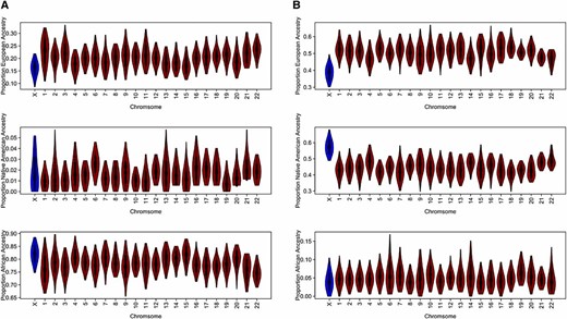
Local ancestry estimates by chromosome. Shown are chromosomal averaged local ancestry estimates for HapMap individuals using the RFMix software. Ancestry was estimated for each marker and then averaged across chromosomes. (A) Estimates for 87 HapMap ASW individuals. (B) Estimates for 86 HapMap MXL individuals. The reference samples for the European and African ancestries were HapMap CEU and YRI individuals, while the HGDP samples from the Americas were references for the Native American ancestry.
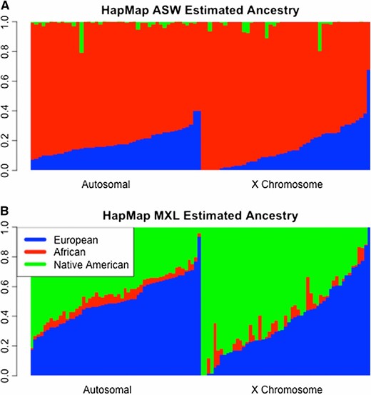
Bar plots of RFMix results. Shown are local ancestry estimates for HapMap individuals using the RFMix software. Each individual is represented by a vertical bar, where the European, African, and Native American ancestries are colored with blue, red, and green, respectively. Left and right panels represent the autosomal and X chromosome averages, respectively. (A) Estimates for 87 HapMap ASW individuals. (B) Estimates for 86 HapMap MXL individuals. The reference samples for the European and African ancestries were HapMap CEU and YRI individuals, while the HGDP samples from the Americas were references for the Native American ancestry.
We calculated the correlation of ancestry proportions across the autosomes and X chromosome for each ancestral subpopulation. The correlations between the autosomal and X chromosome proportions in the European and African ancestries are 0.20 and 0.17, respectively. Interestingly, with a correlation of 0.78, Native American ancestry between the autosomal and X chromosome is the highest despite this ancestry being the least prominent of the three. We find that the high correlation is being driven by two outlier individuals in the ASW with extremely high Native American ancestry (>0.2) on the autosomes and the X compared to the vast majority of ASW individuals who have little to no Native American ancestry. When the two outlier individuals in ASW with high Native American ancestry are excluded, the correlation between Native American ancestry on autosomes and the X chromosome is 0.029, which is similar to the correlation results of the least prominent ancestry in the MXL, as discussed in the next subsection.
HapMap MXL ancestry
From our local ancestry analysis of the 86 HapMap MXL individuals, we found the predominant ancestries to be European and Native American, as expected based on previously reported results (Thornton et al. 2012; Bryc et al. 2015), with African ancestry being quite modest with little variation. Table 2 shows the mean and SD of the average local ancestry estimates by chromosome and averaged across the autosomes within the MXL samples. Interestingly, proportional Native American ancestry is highest on the X chromosome, with a mean of 0.57, while for the autosomes, European ancestry is highest with a mean of 0.51. African ancestry on the autosomes and the X chromosome, however, is quite similar, with mean values of 0.04 and 0.05, respectively. Figure 2B shows violin plots by chromosome of the RFMix local ancestry estimates in the MXL samples. The plots illustrate the marked increase in proportional European ancestry across the autosomes and, correspondingly, a decrease in proportional Native American ancestry on the autosomes compared to the X chromosome. Figure 3B shows bar plots of the ancestral proportions within each individual. The proportion of both European and Native American ancestries on the X chromosome ranges from 0 to 1. The range and variation of the European and Native American ancestries on the X chromosome are larger than those estimated across the autosomes. Furthermore, Native American and European ancestries on the X chromosome are almost perfectly negatively correlated (corr = −0.98). Interestingly, there is one male MXL individual who has an X chromosome that is inferred to be completely Native American derived. The phased RFMix results of this individual’s mother indicate that one of her X chromosomes is entirely Native American derived while her other X chromosome is 69% Native American and 31% European, with five ancestry switches on the chromosome.
We also calculated correlations in ancestry between the average of the autosomes and the X chromosome. European and Native American ancestries have correlations of 0.71 and 0.67, respectively, between the autosomes and the X chromosome. With a correlation of 0.03, there is essentially no correlation in African ancestry between the autosomes and the X in the MXL.
Genome-wide ancestry heterogeneity testing: HapMap MXL and ASW
We applied the CAnD test to the set of 53 unrelated MXL individuals to test for heterogeneity in ancestry across all 23 chromosomes: the 22 autosomes, and the X chromosome. This CAnD test has 22 d.f. under the null hypothesis, and the genome-wide P-values for heterogeneity in African, European, and Native American ancestries are 0.592, 4.01e-05, and 9.57e-06, respectively. To gain insight into which chromosome(s) may be driving the significance of the genome-wide CAnD test for the European and Native American ancestries in the MXL, we used CAnD to test for ancestry differences between each chromosome and the pool of the ancestries of the other 22 chromosomes. Each of these tests has 1 d.f., and Figure 4 shows, by chromosome, the unadjusted (Figure 4A) and Bonferroni-adjusted (Figure 4B) CAnD P-values in the HapMap MXL for each of the three assumed ancestries. Chromosome 7 and the X chromosome have significantly larger proportions of Native American ancestry compared to the pooled Native American mean ancestry of all other chromosomes, at the 0.05 level before adjustment for multiple testing. The X chromosome also has significantly less European ancestry, at the 0.05 level, compared to the pooled autosomes. Chromosome 8 has a larger proportion of African ancestry compared to the pooled ancestry of all other chromosomes. Using a conservative Bonferroni multiple-testing correction, ancestry differences between the X chromosome and the autosomes remain significant for both the European and Native American ancestries in the MXL, while chromosomes 7 and 8 are no longer significant after Bonferroni correction.
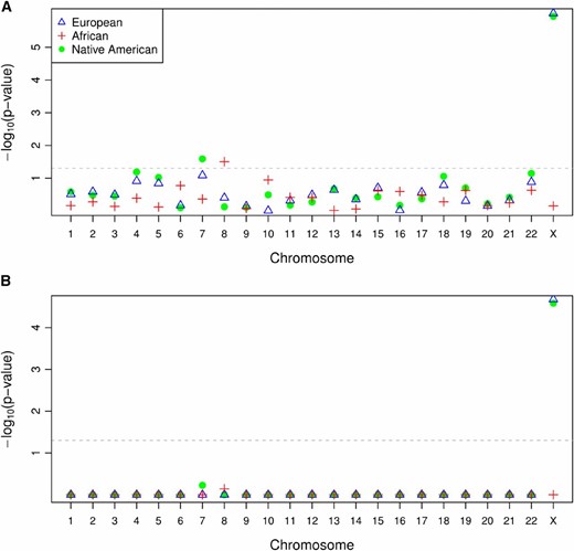
Unadjusted and adjusted P-values from the CAnD test in the HapMap MXL samples. (A and B) Unadjusted (A) and adjusted (B) P-values by chromosome obtained from the CAnD test comparing the estimated ancestry for each chromosome with the mean ancestry of all remaining chromosomes, including the X chromosome, for the African, European, and Native American ancestries in the HapMap MXL samples. The adjusted P-values were calculated using the Bonferroni multiple-testing correction.
We also performed CAnD tests in the MXL excluding the X chromosome, and the overall CAnD test is not significant, with P-values of 0.532, 0.382, and 0.190 corresponding to the African, European, and Native American ancestries, respectively. These results provide additional evidence that differential ancestry on the X chromosome is driving the significant heterogeneity results of the genome-wide CAnD test. We also conducted CAnD tests for ancestry differences for each autosomal chromosome in turn compared to the pool of ancestries from the other autosomes, and none of the autosomal chromosomes are significant after Bonferroni correction (Figure S3).
In an analysis of the 45 unrelated ASW individuals, CAnD did not detect any significant differences in ancestry among the autosomal and X chromosomes. The genome-wide CAnD test for ancestry differences in the ASW had P-values of 0.122, 0.0858, and 0.243 for the African, European, and Native American ancestries, respectively (Figure S2). As previously mentioned, the autosomes and the X chromosome are predominantly African derived in the ASW, and a larger sample size is needed to achieve enough power to detect the smaller ancestry differences among chromosomes in the ASW. Indeed, in much larger population-based samples of African-Americans (Bryc et al. 2010a, 2015), increased African ancestry and decreased European ancestry have been reported for the X chromosome compared to the autosomes.
Assessing ancestry differences between the X and the autosomes: HapMap MXL and ASW
Previous studies have identified significant differences between autosomal and X chromosome ancestry proportions in individuals from admixed populations (Bryc et al. 2015), where these differences have been assessed using a pooled t-test that assumes independence in ancestry among chromosomes. As previously mentioned, CAnD can also be used to test for differences between the X chromosome and the pooled autosomes while appropriately accounting for ancestry correlations among chromosomes within an admixed individual.
Figure 5 shows histograms of the mean difference between the autosomal and X chromosome ancestry proportions for the subsets of 45 unrelated ASW (Figure 5A) and 53 unrelated MXL (Figure 5B) individuals, with a smoothed density line overlaid. The mean difference in European ancestry between the autosomes and the X chromosome is 0.12, and the mean difference for Native American ancestry is −0.13. Based on our simulation studies, we expect to have high power to detect such large differences in ancestry for a sample of this size. For the ASW samples, however, the mean difference between the X chromosome and the autosomes for the two predominant continental ancestries, African and European, is 0.04, which is a much smaller difference than observed for the two predominant ancestries in the MXL. As a result, we expect the power to detect a mean difference in ancestry between the X and the autosomes in the ASW to be much lower, compared to the MXL, for the predominant ancestries.
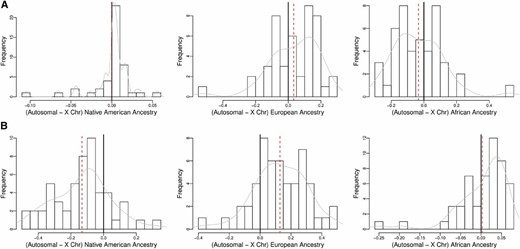
Difference in autosomal and X chromosome ancestry, by subpopulation. Shown are histograms of the difference in autosomal and X chromosome ancestry proportions among the (A) 45 unrelated HapMap ASW and (B) 53 unrelated HapMap MXL samples. The dashed line indicates the mean difference, whereas the solid line indicates zero. A smoothed density line is overlaid on each histogram.
We compared the results of the pooled t-test to a CAnD test with 1 d.f. for detecting differences in ancestry between the X chromosome and the autosomes in the HapMap ASW and MXL. As expected, no significant differences in ancestry were detected in the ASW with either method for any of the three continental ancestries. For the MXL, the pooled t-test identifies significant differences in European ancestry and Native American ancestry between the autosomes and the X chromosome, with a P-value of 0.001 for both analyses. In comparison, the CAnD test P-value is 9.17e-07 for a difference in European ancestry between the autosomes and the X chromosome in the MXL and 1.13e-06 for Native American ancestry, which is more than three orders of magnitude smaller than the P-values for the pooled t-test. There was no significant difference in African ancestry for both methods in the MXL.
Comparison of CAnD results using local vs. global ancestry estimates
We also performed a CAnD analysis in the HapMap MXL and ASW, using global ancestry estimates for each chromosome with the aforementioned FRAPPE method, which takes as input unphased genotype data and assumes independence among genetic markers on a chromosome (Figure S4). Table S1 contains the CAnD results using chromosome-wide ancestry estimates from FRAPPE as well as the previously discussed results from CAnD with local ancestry estimates from the RFMix method, which requires phased genotype data and takes into account LD among SNPs. For the ancestry heterogeneity analysis of the ASW with chromosome-wide ancestry estimates from FRAPPE, no differences in ancestry among chromosomes were detected with CAnD, similar to the CAnD results with local ancestry estimates from RFMix. Interestingly, for the MXL we found that the CAnD results for testing Native American ancestry are slightly more significant when using chromosome-wide ancestry estimates from FRAPPE compared to using local ancestry estimates from RFMix, with P-values of 9.47e-07 and 9.57e-06, respectively. However, this difference is likely due to FRAPPE ignoring LD among SNPs on a chromosome while RFMix incorporates LD in the ancestry estimation procedure. Despite methodological differences, however, inference about heterogeneity in population structure is qualitatively the same when using either local ancestry estimates from RFMix or global ancestry estimates from FRAPPE in the analyses of the ASW and MXL, as can be seen in Table S1.
We also compared autosomal-wide and X chromosome ancestry estimates from RFMix and FRAPPE, using genotype data for the HapMap MXL and ASW population samples. Table 3 shows the correlation of the ancestry estimates from the methods for each ancestral subpopulation. For the two predominant ancestries in the MXL (European and Native American) and ASW (African and European), the correlations between the ancestry estimates for the autosomes from RFMix and FRAPPE are all >0.99 and are ≥0.95 for the X chromosome. As previously mentioned, there is very little Native American ancestry and African ancestry in the ASW and MXL, respectively. Nevertheless, with a correlation of 0.99, Native American ancestry estimates on the autosomes are nearly perfectly correlated between RFMix and FRAPPE, and the correlation between the estimates is 0.90 for Native American ancestry on the X chromosome in the ASW. For proportional African ancestry in the MXL, the correlation between the two estimates is 0.893 for the autosomes and 0.93 for the X chromosome. So, for the predominant ancestries in the MXL and ASW, there appears to be little difference in estimating autosomal ancestries with FRAPPE or averaging local ancestry estimates from RFMix. There is high concordance between the methods for the predominant ancestry in ASW and MXL for the X chromosome as well. In general, there is less concordance between the methods when estimating proportional ancestries from populations with relatively small contributions to the admixed population, and local ancestry estimates, such as RFMix, are likely more accurate in inferring low levels of ancestral contribution than global ancestry methods, such as FRAPPE.
Correlation of ancestry estimates
| Autosomal | X chromosome | |||
|---|---|---|---|---|
| Ancestry | ASW | MXL | ASW | MXL |
| African | 0.9990 | 0.8932 | 0.9697 | 0.9256 |
| European | 0.9979 | 0.9935 | 0.9548 | 0.9878 |
| Native American | 0.9963 | 0.9940 | 0.9001 | 0.9898 |
| Autosomal | X chromosome | |||
|---|---|---|---|---|
| Ancestry | ASW | MXL | ASW | MXL |
| African | 0.9990 | 0.8932 | 0.9697 | 0.9256 |
| European | 0.9979 | 0.9935 | 0.9548 | 0.9878 |
| Native American | 0.9963 | 0.9940 | 0.9001 | 0.9898 |
Shown is correlation between ancestry estimates from RFMix and FRAPPE, stratified by autosomal and X chromosome estimates, in each of the population samples.
| Autosomal | X chromosome | |||
|---|---|---|---|---|
| Ancestry | ASW | MXL | ASW | MXL |
| African | 0.9990 | 0.8932 | 0.9697 | 0.9256 |
| European | 0.9979 | 0.9935 | 0.9548 | 0.9878 |
| Native American | 0.9963 | 0.9940 | 0.9001 | 0.9898 |
| Autosomal | X chromosome | |||
|---|---|---|---|---|
| Ancestry | ASW | MXL | ASW | MXL |
| African | 0.9990 | 0.8932 | 0.9697 | 0.9256 |
| European | 0.9979 | 0.9935 | 0.9548 | 0.9878 |
| Native American | 0.9963 | 0.9940 | 0.9001 | 0.9898 |
Shown is correlation between ancestry estimates from RFMix and FRAPPE, stratified by autosomal and X chromosome estimates, in each of the population samples.
Assortative mating for ancestry in the HapMap MXL
Sex-specific patterns of nonrandom mating at the time of or since admixture can result in ancestry differences between the autosomes and the X chromosome in an admixed population. Motivated by the CAnD results where significant heterogeneity between the autosomes and the X chromosome were detected in the MXL, we investigated evidence of assortative mating between pairs of individuals who are reported to have least one offspring. There are 24 such mate pairs; however, we excluded 3 mate pairs due to cryptic relatedness (as previously discussed), resulting in a subset of 21 independent MXL mate pairs included in the assortative mating analysis.
We used an empirical distribution to assess whether the observed correlations of ancestry on the autosomes and the X chromosome between mate pairs are significantly different from what would be expected under the null hypothesis of random mating. In particular, we randomly permuted the MXL mate pairs 5000 times, and for each of the 5000 permutations, we calculated the correlations in ancestry between the random mate pairs for each of the three continental ancestries (European, Native American, and African). The correlations in ancestry between mate pairs for the autosomes and the X chromosome were then used to construct empirical distributions under the null hypothesis of random mating in the MXL. The empirical distributions of ancestry correlations among mate pairs are centered ∼0 under random mating, with a standard deviation ∼0.2 for each of the three ancestries (Figure S5).
We first tested the null hypothesis vs. an alternative hypothesis of assortative mating for ancestry, using the observed correlations among mate pairs and the empirical null distributions. Table 4 shows the P-values for the autosomal and X chromosome correlations of African, European, and Native American ancestry proportions calculated from the 21 MXL mate pairs. There is significant evidence of assortative mating for European and Native American ancestries on the autosomes in the HapMap MXL, with corresponding P-values of 0.015 and 0.017, respectively. There is also significant evidence for assortative mating based on European and Native American ancestry on the X chromosome, with P-values of 0.011 and 0.007, respectively. The P-values remain significant, even after Bonferroni correction for testing three ancestries. There is no significant evidence of assortative mating for African ancestry for both the autosomes and the X chromosomes (P = 0.26 and 0.14, respectively). A two-sided test of the null hypothesis of random mating vs. an alternative hypothesis of nonrandom, e.g., assortative or disassortative mating, can also be conducted. The P-values for this test are given in Table 4 and are roughly twice the assortative mating P-values. We also performed permutation tests to assess evidence of assortative and nonrandom mating for 11 HapMap ASW mate pairs with a documented offspring. No significant evidence of assortative mating in the ASW was detected, and ASW P-values for the three continental ancestries are given in Table 4.
Ancestry correlation among mate pairs
| HapMap ASW | HapMap MXL | |||||
|---|---|---|---|---|---|---|
| Chromosome Type | African | European | Native American | African | European | Native American |
| Autosomal | ||||||
| Assortative mating | 0.365 | 0.388 | 0.234 | 0.139 | 0.015 | 0.017 |
| Nonrandom mating | 0.871 | 0.888 | 0.532 | 0.268 | 0.028 | 0.032 |
| X chromosome | ||||||
| Assortative mating | 0.842 | 0.788 | 0.564 | 0.256 | 0.011 | 0.007 |
| Nonrandom mating | 1.000 | 1.000 | 1.000 | 0.530 | 0.024 | 0.013 |
Shown are P-values detecting assortative or disassortative mating for ancestry among 11 HapMap ASW and 21 HapMap MXL mate pairs, calculated on the autosomes and the X chromosome separately. The P-values are calculated from the empirical distribution created from sampling 5000 mate pairs at random. Results presented under “assortative mating” tested the hypothesis of no assortative mating, while “nonrandom mating” tested the hypothesis of neither assortative nor disassortative mating.
| HapMap ASW | HapMap MXL | |||||
|---|---|---|---|---|---|---|
| Chromosome Type | African | European | Native American | African | European | Native American |
| Autosomal | ||||||
| Assortative mating | 0.365 | 0.388 | 0.234 | 0.139 | 0.015 | 0.017 |
| Nonrandom mating | 0.871 | 0.888 | 0.532 | 0.268 | 0.028 | 0.032 |
| X chromosome | ||||||
| Assortative mating | 0.842 | 0.788 | 0.564 | 0.256 | 0.011 | 0.007 |
| Nonrandom mating | 1.000 | 1.000 | 1.000 | 0.530 | 0.024 | 0.013 |
Shown are P-values detecting assortative or disassortative mating for ancestry among 11 HapMap ASW and 21 HapMap MXL mate pairs, calculated on the autosomes and the X chromosome separately. The P-values are calculated from the empirical distribution created from sampling 5000 mate pairs at random. Results presented under “assortative mating” tested the hypothesis of no assortative mating, while “nonrandom mating” tested the hypothesis of neither assortative nor disassortative mating.
Ancestry equilibrium on the X chromosome under random mating after an initial admixture event
We also investigated the number of generations required for males and females to reach ancestry equilibrium on the X chromosome in a randomly mating population. We considered the setting where there is admixing between two ancestral populations and where mate pairs at the initial admixture event consist of males with ancestry entirely from one population and females with ancestry derived from the other population. We computed proportional ancestry for each generation, assuming random mating after an initial admixing event between founder females and males under the extreme discordant ancestry setting between the two sexes at the time of admixture. Figure 6 shows the proportion of ancestry by generation in the admixed population for males and females. We find that an equilibrium of one-half is reached for autosomal ancestry in males and females in the first generation. Proportional ancestry on the X chromosome for both males and females tends to two-thirds and one-third of the founder female and male ancestries, respectively, where this equilibrium is achieved around eight generations after the initial admixing event. This equilibrium result is not surprising since females contribute two-thirds of the X chromosomes in a population. Recent work (Goldberg and Rosenberg 2015) identified a similar result (although the initial ancestry proportions at the time of admixture were not as extreme as what we consider here) and showed that the two-thirds and one-third ancestry equilibrium on the X does not hold if admixing is ongoing. Nevertheless, whether there is a single admixture event or ongoing admixture, the X chromosome and the autosomal chromosomes are not expected to have the same ancestry distribution at equilibrium in a randomly mating admixed population when the ancestry distribution for founder males is different from that for founder females at the time of the admixture event(s).
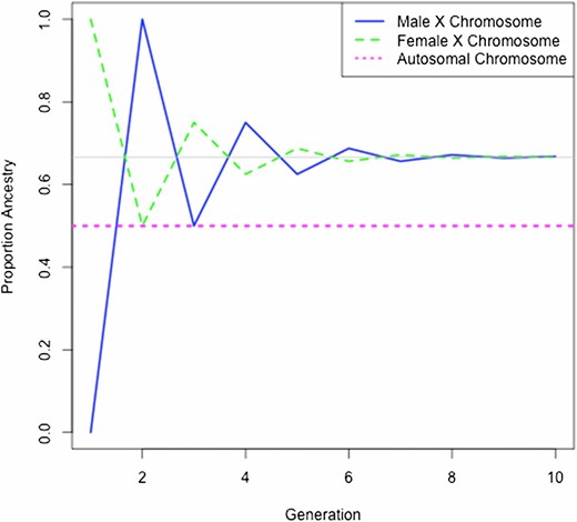
Ancestry proportions by generation under random mating. Shown is the proportion of ancestry for the autosomes and the X chromosome by sex, assuming females and males have opposite ancestries at the initial admixture event. After the initial admixture event, random mating is assumed. The gray line shows the equilibrium proportions on the X chromosome.
Discussion
Systematic ancestry differences at genomic loci may arise in recently admixed populations as a result of selection and ancestry-related assortative mating. Here, we developed the CAnD method for detecting heterogeneity in population structure across the genome in populations with admixed ancestry. CAnD uses inferred ancestry from genotyping data to identify chromosomes harboring genomic loci that have significantly different contributions from the underlying ancestral populations from what is expected based on genome-wide ancestry. The CAnD method takes into account correlated ancestries among chromosomes within individuals for both valid testing and improved power for detecting heterogeneity in population structure across the genome. Additional features of the CAnD method include (1) allowing for genetic data from the X chromosome to be included in a heterogeneity analysis and (2) flexibility of the method that allows for heterogeneity testing between subsets of chromosomes in the genome, such as the X chromosome vs. the pooled autosomes.
We performed simulation studies with admixture, using real genotype data from HapMap. We demonstrated that CAnD is properly calibrated with appropriate type I error under different significance levels. We also showed that the CAnD test has higher power to detect heterogeneity in ancestry genome-wide chromosomes than an ANOVA test that does not account for correlations in ancestry among chromosomes.
We applied the CAnD method to the HapMap MXL population sample where significant heterogeneity in European ancestry and Native American ancestry was detected across the genome (autosomal chromosomes and the X chromosome), with P-values of 4e-05 and 1e-05, respectively. A secondary analysis showed that the heterogeneity in ancestry across the MXL genomes detected by CAnD was largely due to elevated Native American ancestry and a deficit of European ancestry on the X chromosomes. These results are consistent with previous reports for U.S. Hispanic/Latinos (Bryc et al. 2015) and Latin Americans (Bryc et al. 2010b), where it has been suggested that the X vs. autosomal ancestry differences are likely due to sex-specific patterns of gene flow in which European male colonists contributed substantially more genetic material than European females at the time of admixture. There was no significant evidence of genetic heterogeneity with CAnD among HapMap ASW chromosomes and no significant differences in ancestry between the pooled autosomes and the X chromosome were detected. The autosomal chromosomes and the X chromosome in the ASW are largely African derived, and a much larger sample is required to have adequate power for detecting chromosomal ancestry differences in this population.
The CAnD method can incorporate estimates of local ancestry at specific locations across the genomes using software such as RFMix, as well as chromosome-wide ancestry estimates using global ancestry estimation software such as FRAPPE or ADMIXTURE. We compared the CAnD results for the HapMap MXL when using local ancestry estimates from RFMix, which requires phased genotype data, to the results when using chromosomal ancestry estimates with FRAPPE where unphased genotype data were used. Significant evidence of ancestry heterogeneity was detected with CAnD when using either local ancestry estimates from RFMix or chromosome-wide ancestry estimates from FRAPPE.
We also investigated the number of generations required for ancestry on the X chromosome to reach equilibrium in males and females after a single admixing event with two populations. In the most extreme setting where all males are from one population and all females are from the other population at the time of admixture, approximately 8 generations are required under random mating between males and females to reach ancestry equilibrium on the X. Estimates of the number of generations since admixture in the Mexican population (Johnson et al. 2011) range from 10 to 15, so it is reasonable to assume that equilibrium on the X chromosome for males and females should have been reached in the Mexican population if mating in this population is completely at random. Previous studies (Risch et al. 2009; Sebro et al. 2010), however, have shown evidence of nonrandom mating in Mexican populations. In the HapMap MXL, we detected significant evidence of assortative mating among mate pairs that produced an offspring, where the correlation of European and Native American ancestries on both the autosomes and the X chromosome is significantly higher for mate pairs than what would be expected under the null hypothesis of a random mating population. Evaluating differences in ancestry on the X chromosome between males and females may potentially be a useful tool for the detection of nonrandom mating in recently admixed populations, since under the most extreme setting of discordant ancestry between males and females at the time of admixture we find that that there should be no difference in ancestry on the X chromosome between males and females after 8 generations of random mating.
In this article, we proposed CAnD to identify heterogeneity in genome-wide ancestry. Secondary analyses can also be conducted with CAnD to identify specific chromosomes that have ancestry distributions that are significantly different from those of all other chromosomes. If local ancestry estimates are available, CAnD can also potentially be used as a fine-mapping tool for identifying chromosomal regions that may be under selection. For example, using a sliding-window approach, the CAnD test could be used to test regions on a chromosome that have systematic ancestry differences compared to the rest of the genome. This is future work to be considered.
Appendix A
Derivation of the Covariance Matrix for the CAnD Multivariate Statistic
Consider a set with m chromosomes and let be the previously defined multivariate vector of length m for the CAnD test for a sample with n independent individuals, where Below we derive an estimate for the covariance matrix of for testing the null hypothesis of heterogeneity in ancestry among m chromosomes in
Appendix B
CAnD Multivariate Statistic in Matrix Form
The multivariate statistic can be written as where is a length m vector of subpopulation k proportional ancestries for each of individual i’s chromosomes in and is an matrix with diagonal elements equal to 1 and off-diagonal elements equal to The rank of is since each row of the matrix can be written as a linear combination of the other rows. From this result, it follows that the corresponding CAnD statistic given in Equation 2 follows a distribution with d.f.
Acknowledgments
The authors thank the two anonymous reviewers for helpful comments that improved the manuscript. This work was supported by National Institutes of Health grants K01 CA148958 (to T.A.T.) and P01 HG0099568 (to C.M. and T.A.T.) and Hispanic Community Health Study/Study of Latinos Genetic Analysis Center grant HHSN268201300005C (to C.M. and T.A.T.).
Footnotes
Communicating editor: E. Eskin
Supplemental material is available online at www.genetics.org/lookup/suppl/doi:10.1534/genetics.115.184184/-/DC1.
Literature Cited
Xu, X., L. Tian, and L. J. Wei, 2003 Combining dependent tests for linkage or association across multiple phenotypic traits. Biostatistics 4: 223–229.
