The Next Generation of Molecular Markers From Massively Parallel Sequencing of Pooled DNA Samples

Futschik, Andreas; Schlötterer, Christian

doi:10.1534/genetics.110.114397

Abstract

Next generation sequencing (NGS) is about to revolutionize genetic analysis. Currently NGS techniques are mainly used to sequence individual genomes. Due to the high sequence coverage required, the costs for population-scale analyses are still too high to allow an extension to nonmodel organisms. Here, we show that NGS of pools of individuals is often more effective in SNP discovery and provides more accurate allele frequency estimates, even when taking sequencing errors into account. We modify the population genetic estimators Tajima's π and Watterson's θ to obtain unbiased estimates from NGS pooling data. Given the same sequencing effort, the resulting estimators often show a better performance than those obtained from individual sequencing. Although our analysis also shows that NGS of pools of individuals will not be preferable under all circumstances, it provides a cost-effective approach to estimate allele frequencies on a genome-wide scale.

NEXT generation sequencing (NGS) is about to revolutionize biology. Through a massive parallelization, NGS provides an enormous number of reads, which permits sequencing of entire genomes at a fraction of the costs for Sanger sequencing. Hence, for the first time it has become feasible to obtain the complete genomic sequence for a large number of individuals. For several organisms, including humans, Drosophila melanogaster, and Arabidopsis thaliana, large resequencing projects are well on their way. Nevertheless, despite the enormous cost reduction, genome sequencing on a population scale is still out of reach for the budget of most laboratories. The extraction of as much statistical information as possible at cost as low as possible has therefore already attracted considerable interest. See, for instance, Jiang et al. (2009) for the modeling of sequencing errors and Erlich et al. (2009) for the efficient tagging of sequences.

Current genome-wide resequencing projects collect the sequences individual by individual. To obtain full coverage of the entire genome and to have high confidence that all heterozygous sites were discovered, it is required that genomes are sequenced at a sufficiently high coverage. As many of the reads provide only redundant information, cost could be reduced by a more effective sampling strategy.

In this report, we explore the potential of DNA pooling to provide a more cost-effective approach for SNP discovery and genome-wide population genetics. Sequencing a large pool of individuals simultaneously keeps the number of redundant DNA reads low and provides thus an economic alternative to the sequencing of individual genomes. On the other hand, more care has to be taken to establish an appropriate control of sequencing errors. Obviously haplotype information is not available from pooling experiments, but this will often be outweighed by the increased accuracy in population genetic inference.

Focusing on biallelic loci, our analysis shows that with sufficiently large pool sizes, pooling usually outperforms the separate sequencing of individuals, both for estimating allele frequencies and for inference of population genetic parameters. When sequencing errors are not too common, pooling seems also to be a good choice for SNP detection experiments. To avoid the additional challenges encountered with individual sequencing of diploid individuals, we compare pooling with individual sequencing of haploid individuals. See Lynch (2008, 2009) for a discussion of next generation sequencing of diploid individuals. Our results for the pooling experiments should be also applicable to a diploid setting, as we are just merging pools of size 2 to a larger pool in this case, leading to a pool size of n = 2n_d for n_d diploid individuals. In the methods section, we derive several mathematical expressions that permit us to compare pooling with separate sequencing of individuals. These formulas are then applied in the results section to illustrate the differences in accuracy between the approaches. A reader who is interested only in the actual differences under several scenarios might therefore want to move directly to the results section.

METHODS

Throughout, we consider an individual sequencing project where k individuals are sequenced each with an expected coverage λ, by which we mean that any given locus is sequenced λ times on average. For a comparable pooling experiment that involves the same amount of sequencing effort, the expected coverage will then be kλ; i.e., any particular locus will be read kλ times on average from the pool consisting of n individuals. In practice, one might for instance sequence each of the k individuals on a separate Illumina lane with coverage λ. With the same sequencing effort, the pool could be sequenced on k lanes simultaneously, leading to a total coverage of kλ.

For the convenience of the reader, we summarize our notation in Table 1.

TABLE 1

Open in new tab

Description of our notation

Symbol or notation	Description
k	No. of haploid individuals used for separate sequencing
λ	Expected no. of times a locus is read for an individual using separate sequencing
n	Size of the pool in a pooling experiment
J	Random no. of individuals for which reads are actually available at a particular locus with individual sequencing (J ≤ k)
M	Random no. of reads for a particular locus in a pooling experiment [E(M) = kλ]
p	Relative frequency of the allele of interest in the population
F_(P)(b, γ)	Poisson cumulative distribution function (⁠ \(F_{(\mathrm{P})}(b,{\,}\mathrm{{\gamma}}){=}{\sum}_{i{=}0}^{b}(\mathrm{{\gamma}}^{i}{\,}/i!)\mathrm{exp}({-}\mathrm{{\gamma}})\) ⁠)
F_(B)(x, M, p)	Binomial cumulative distribution function \((F_{(\mathrm{B})}(x,{\,}M,{\,}p){=}{\sum}_{i{=}0}^{x}{[}\begin{array}{l}M\\i\end{array}{]}p^{i}(1{-}p)^{M{-}i})\)
\(\mathrm{{\hat{{\theta}}}}_{\mathrm{{\pi}}}^{(b){\ast}}\)	Bias-corrected version of Tajima's π for a pooling experiment when the minor allele frequency is required to be at least b. For b = 1, \(\mathrm{{\hat{{\theta}}}}_{\mathrm{{\pi}}}^{(b){\ast}}{=}\mathrm{{\hat{{\theta}}}}_{\mathrm{{\pi}}}^{{\ast}}\)
\(\mathrm{{\hat{{\theta}}}}_{\mathrm{W}}^{(b){\ast}}\)	Bias-corrected version of Watterson's θ for a pooling experiment when the minor allele frequency is required to be at least b ≥ 1

Symbol or notation	Description
k	No. of haploid individuals used for separate sequencing
λ	Expected no. of times a locus is read for an individual using separate sequencing
n	Size of the pool in a pooling experiment
J	Random no. of individuals for which reads are actually available at a particular locus with individual sequencing (J ≤ k)
M	Random no. of reads for a particular locus in a pooling experiment [E(M) = kλ]
p	Relative frequency of the allele of interest in the population
F_(P)(b, γ)	Poisson cumulative distribution function (⁠ \(F_{(\mathrm{P})}(b,{\,}\mathrm{{\gamma}}){=}{\sum}_{i{=}0}^{b}(\mathrm{{\gamma}}^{i}{\,}/i!)\mathrm{exp}({-}\mathrm{{\gamma}})\) ⁠)
F_(B)(x, M, p)	Binomial cumulative distribution function \((F_{(\mathrm{B})}(x,{\,}M,{\,}p){=}{\sum}_{i{=}0}^{x}{[}\begin{array}{l}M\\i\end{array}{]}p^{i}(1{-}p)^{M{-}i})\)
\(\mathrm{{\hat{{\theta}}}}_{\mathrm{{\pi}}}^{(b){\ast}}\)	Bias-corrected version of Tajima's π for a pooling experiment when the minor allele frequency is required to be at least b. For b = 1, \(\mathrm{{\hat{{\theta}}}}_{\mathrm{{\pi}}}^{(b){\ast}}{=}\mathrm{{\hat{{\theta}}}}_{\mathrm{{\pi}}}^{{\ast}}\)
\(\mathrm{{\hat{{\theta}}}}_{\mathrm{W}}^{(b){\ast}}\)	Bias-corrected version of Watterson's θ for a pooling experiment when the minor allele frequency is required to be at least b ≥ 1

TABLE 1

Open in new tab

Description of our notation

Symbol or notation	Description
k	No. of haploid individuals used for separate sequencing
λ	Expected no. of times a locus is read for an individual using separate sequencing
n	Size of the pool in a pooling experiment
J	Random no. of individuals for which reads are actually available at a particular locus with individual sequencing (J ≤ k)
M	Random no. of reads for a particular locus in a pooling experiment [E(M) = kλ]
p	Relative frequency of the allele of interest in the population
F_(P)(b, γ)	Poisson cumulative distribution function (⁠ \(F_{(\mathrm{P})}(b,{\,}\mathrm{{\gamma}}){=}{\sum}_{i{=}0}^{b}(\mathrm{{\gamma}}^{i}{\,}/i!)\mathrm{exp}({-}\mathrm{{\gamma}})\) ⁠)
F_(B)(x, M, p)	Binomial cumulative distribution function \((F_{(\mathrm{B})}(x,{\,}M,{\,}p){=}{\sum}_{i{=}0}^{x}{[}\begin{array}{l}M\\i\end{array}{]}p^{i}(1{-}p)^{M{-}i})\)
\(\mathrm{{\hat{{\theta}}}}_{\mathrm{{\pi}}}^{(b){\ast}}\)	Bias-corrected version of Tajima's π for a pooling experiment when the minor allele frequency is required to be at least b. For b = 1, \(\mathrm{{\hat{{\theta}}}}_{\mathrm{{\pi}}}^{(b){\ast}}{=}\mathrm{{\hat{{\theta}}}}_{\mathrm{{\pi}}}^{{\ast}}\)
\(\mathrm{{\hat{{\theta}}}}_{\mathrm{W}}^{(b){\ast}}\)	Bias-corrected version of Watterson's θ for a pooling experiment when the minor allele frequency is required to be at least b ≥ 1

Symbol or notation	Description
k	No. of haploid individuals used for separate sequencing
λ	Expected no. of times a locus is read for an individual using separate sequencing
n	Size of the pool in a pooling experiment
J	Random no. of individuals for which reads are actually available at a particular locus with individual sequencing (J ≤ k)
M	Random no. of reads for a particular locus in a pooling experiment [E(M) = kλ]
p	Relative frequency of the allele of interest in the population
F_(P)(b, γ)	Poisson cumulative distribution function (⁠ \(F_{(\mathrm{P})}(b,{\,}\mathrm{{\gamma}}){=}{\sum}_{i{=}0}^{b}(\mathrm{{\gamma}}^{i}{\,}/i!)\mathrm{exp}({-}\mathrm{{\gamma}})\) ⁠)
F_(B)(x, M, p)	Binomial cumulative distribution function \((F_{(\mathrm{B})}(x,{\,}M,{\,}p){=}{\sum}_{i{=}0}^{x}{[}\begin{array}{l}M\\i\end{array}{]}p^{i}(1{-}p)^{M{-}i})\)
\(\mathrm{{\hat{{\theta}}}}_{\mathrm{{\pi}}}^{(b){\ast}}\)	Bias-corrected version of Tajima's π for a pooling experiment when the minor allele frequency is required to be at least b. For b = 1, \(\mathrm{{\hat{{\theta}}}}_{\mathrm{{\pi}}}^{(b){\ast}}{=}\mathrm{{\hat{{\theta}}}}_{\mathrm{{\pi}}}^{{\ast}}\)
\(\mathrm{{\hat{{\theta}}}}_{\mathrm{W}}^{(b){\ast}}\)	Bias-corrected version of Watterson's θ for a pooling experiment when the minor allele frequency is required to be at least b ≥ 1

SNP detection:

A SNP is detected at a site if the site is polymorphic, i.e., if at least two alleles A and a are found in the sequenced sample. We consider SNP detection both in the context of pooling experiments and for individual sequencing. To assess the performance of these two competing scenarios, we look both at the power and at the probability of falsely calling a SNP due to sequencing errors.

Generally speaking, an experimental design that provides high power while keeping the probability of incorrectly detecting a SNP small is preferable. When individuals are sequenced separately, the probability of sequencing errors being interpreted as true SNPs can be reduced by a sufficiently high expected coverage if the genotype of an individual is inferred by the majority of reads. Note that in the case of diploid individuals, the distinction between sequencing errors and true SNPs is significantly more complicated. In pooling experiments, a simple way to control the probability of falsely detecting SNPs both in the haploid and in the diploid case is to require a certain minimum number of reads for the minor allele to call a SNP. We extend work by Eberle and Kruglyak (2000) on SNP detection and derive both the power and error rates for pooling experiments and for separate sequencing.

Separate sequencing of individuals:

Let M_A (M_a) denote the number of times allele A (a) is sequenced. Given that exactly L_A = l of k individuals in the sample have an allele of type A, the probability of detecting polymorphism is equal to the probability of reading at least one of the A and one of the remaining a alleles in the sample. Assuming that for each individual the number of reads at a particular locus is Poisson distributed with parameter λ, the probability of not covering the SNP locus for an individual is exp(–λ). This leads to the probability

\[q_{\mathrm{c}}(l,k,\mathrm{{\lambda}}):{=}(1{-}{[}\mathrm{exp}({-}\mathrm{{\lambda}}){]}^{l})(1{-}{[}\mathrm{exp}({-}\mathrm{{\lambda}}){]}^{k{-}l})\]

for getting at least one “A” and one “a” read. Note that for larger values of λ, this probability is nearly one, except for l = 0 or l = k, where q_c(l, k, λ) = 0. Suppose now that our population size N is fairly large and that the relative frequency of allele A is p in the population. Then, by conditioning on the number l of A alleles in the sample, the probability of detecting a SNP is approximately

\[q(p,k,\mathrm{{\lambda}}){=}{{\sum}_{l{=}1}^{k{-}1}}q_{\mathrm{c}}(l,k,\mathrm{{\lambda}})\left(\begin{array}{l}k\\l\end{array}\right)p^{l}(1{-}p)^{k{-}l}.\]

(1)

For large values of λ, we obtain that

\[q(p,k,\mathrm{{\lambda}}){\approx}1{-}p^{k}{-}(1{-}p)^{k}.\]

(2)

We now derive the probability of wrongly detecting a SNP due to sequencing errors. A natural way to proceed for individual sequencing is to assume that the most frequently read base for an individual is the true one. The probability that this leads to the wrong decision depends on the number of reads available for the locus under investigation, as well as the probability ε that a single read for a given base is incorrect and furthermore on whether the errors are independent. Concerning the dependence of the reading errors, we consider two extreme scenarios. The first, more pessimistic, scenario assumes complete dependence such that sequencing errors at a given position always lead to the same incorrect base. The second assumes independent errors such that each sequencing error leads to an independently chosen wrong base. In this situation, we assume furthermore that the three possible wrong bases are chosen with the same probability. We expect the actual error probabilities somewhere between these scenarios.

For the dependent case, we obtain by conditioning on the (Poisson) number of reads for an individual at a locus

\begin{eqnarray*}&&q_{\mathrm{e}}^{(\mathrm{d})}(k,\mathrm{{\lambda}},\mathrm{{\varepsilon}})\\&&{=}1{-}\left(1{-}{{\sum}_{r{\geq}1}}\left[{{\sum}_{i{>}r/2}}\left(\begin{array}{l}r\\i\end{array}\right)\mathrm{{\varepsilon}}^{i}(1{-}\mathrm{{\varepsilon}})^{(r{-}i)}\right]\frac{\mathrm{{\lambda}}^{r}}{r!}\mathrm{exp}({-}\mathrm{{\lambda}})\right)^{k}.\end{eqnarray*}

(3)

In the independent case, an error is made by choosing one of the three incorrect bases at random, each with probability ε/3. The probability of falsely detecting a SNP is

\begin{eqnarray*}&&q_{\mathrm{e}}^{(\mathrm{i})}(k,\mathrm{{\lambda}},\mathrm{{\varepsilon}})\\&&{=}1{-}\left(1{-}{{\sum}_{r{\geq}1}}\left[3{{\sum}_{i{>}r/2}}\left(\begin{array}{l}r\\i\end{array}\right)\left(\frac{\mathrm{{\varepsilon}}}{3}\right)^{i}(1{-}\frac{\mathrm{{\varepsilon}}}{3})^{(r{-}i)}\right]\frac{\mathrm{{\lambda}}^{r}}{r!}\mathrm{exp}({-}\mathrm{{\lambda}})\right)^{k}.\end{eqnarray*}

(4)

The resulting error probabilities can be made very small by ensuring a coverage λ that is large enough. Obviously a more sophisticated rule will be needed when sequencing diploid individuals.

Pooling experiment:

We now assume that a pooled sample of size n is sequenced with the same expected total number kλ of reads per locus as for separate sequencing. Let

\(F_{(\mathrm{P})}(b,\mathrm{{\gamma}}){=}{\sum}_{i{=}0}^{b}(\mathrm{{\gamma}}^{i}/i!)\mathrm{exp}({-}\mathrm{{\gamma}})\)

denote the probability that a Poisson random variable with parameter γ is at most b. Given a frequency L_A = l of A alleles in the pool, we obtain the probability of reading at least one A and one a allele as

\[\left(1{-}F_{(\mathrm{P})}\left(0,\frac{lk\mathrm{{\lambda}}}{n}\right)\right)\left(1{-}F_{(\mathrm{P})}\left(0,\frac{(n{-}l)k\mathrm{{\lambda}}}{n}\right)\right).\]

(5)

Now this leads to the probability of detecting a SNP,

\begin{eqnarray*}&&{{\sum}_{l{=}1}^{n{-}1}}\left(1{-}F_{(\mathrm{P})}\left(0,\frac{lk\mathrm{{\lambda}}}{n}\right)\right)\left(1{-}F_{(\mathrm{P})}\left(0,\frac{(n{-}l)k\mathrm{{\lambda}}}{n}\right)\right)\left(\begin{array}{l}n\\l\end{array}\right)\\&&{\times}p^{l}(1{-}p)^{n{-}l},\end{eqnarray*}

(6)

which occurs with a proportion p in the population.

As sequencing errors are common in NGS, they are easily confounded with low-frequency alleles. A common strategy to reduce the high probability of sequencing errors is to consider only SNPs that are detected in at least b reads. Requiring a minimum number b of reads in our context, the probability of detecting a SNP changes to

\begin{eqnarray*}&&{{\sum}_{l{=}1}^{n{-}1}}\left(1{-}F_{(\mathrm{P})}\left(b{-}1,\frac{lk\mathrm{{\lambda}}}{n}\right)\right)\left(1{-}F_{(\mathrm{P})}\left(b{-}1,\frac{(n{-}l)k\mathrm{{\lambda}}}{n}\right)\right)\left(\begin{array}{l}n\\l\end{array}\right)\\&&{\times}p^{l}(1{-}p)^{n{-}l}.\end{eqnarray*}

(7)

As with individual sequencing, we again derive the probability of wrongly detecting a SNP under two scenarios for the sequencing errors.

In the dependent scenario, the probability of wrong SNP detection equals the probability

\begin{eqnarray*}&&p_{\mathrm{e}}^{(\mathrm{d})}(k,{\,}\mathrm{{\lambda}},{\,}\mathrm{{\varepsilon}},{\,}b)\\&&{=}(1{-}F_{(\mathrm{P})}(b{-}1,{\,}\mathrm{{\lambda}}k\mathrm{{\varepsilon}}))\left[1{-}F_{(\mathrm{P})}(0,{\,}\mathrm{{\lambda}}k(1{-}\mathrm{{\varepsilon}}))\right]\end{eqnarray*}

(8)

of making at least b sequencing errors and getting at least one correct read. If the expected number of reads λk is fairly large, the term 1 − F_(P)(0, λk(1 − ε)) is very close to one and can be omitted without changing the results much. With independent sequencing errors, an upper bound for the probability of falsely detecting a SNP is given by

\[p_{\mathrm{e}}^{(\mathrm{i})}(k,{\,}\mathrm{{\lambda}},{\,}\mathrm{{\varepsilon}},{\,}b){=}3\left(1{-}F_{(\mathrm{P})}\left(b{-}1,{\,}\frac{\mathrm{{\lambda}}k\mathrm{{\varepsilon}}}{3}\right)\right).\]

(9)

Allele frequency inference:

We consider a locus with expected relative frequency p in the population. Suppose first that the individuals are sequenced separately with an expected coverage of λ. Then the probability that a specific locus is read for J = j of the k individuals is

\[r_{j,k}:{=}(\begin{array}{l}k\\j\end{array})(1{-}e^{{-}\mathrm{{\lambda}}})^{j}e^{{-}(k{-}j)\mathrm{{\lambda}}}.\]

Given that reads are available for J = j of the k individuals, the relative frequency of A alleles is R_c := M_A/j. The variance of R_c can be obtained as

\begin{eqnarray*}&&\mathrm{Var}(R_{\mathrm{c}})\\&&{=}\mathrm{Var}\left(\frac{M_{A}}{J}\right){=}\mathbf{\mathrm{E}}\left(\mathrm{Var}\left[\frac{M_{A}}{J}\mathrm{{\vert}}J\right]\right){+}\mathrm{Var}\left(\mathbf{\mathrm{E}}\left[\frac{M_{A}}{J}\mathrm{{\vert}}J\right]\right).\end{eqnarray*}

Now given J, M_A is binomial B(J, p) distributed and

\(\mathrm{Var(}(M_{A}/J)\mathrm{{\vert}}J){=}p(1{-}p)/J\)

⁠. This leads to

\[\mathbf{\mathrm{E}}\left(\mathrm{Var}\left[\frac{M_{A}}{J}\mathrm{{\vert}}J\right]\right){=}\mathbf{\mathrm{E}}(\frac{1}{J})p(1{-}p).\]

Furthermore

\(\mathbf{\mathrm{E}}{[}(M_{A}/J)\mathrm{{\vert}}J{]}{=}p\)

and therefore

\(\mathrm{Var}(\mathbf{\mathrm{E}}{[}(M_{A}/J)\mathrm{{\vert}}J{]}){=}0\)

⁠. Together

\[\mathrm{Var}(R_{\mathrm{c}}){=}p(1{-}p)\mathbf{\mathrm{E}}\left(\frac{1}{J}\right){\geq}\frac{p(1{-}p)}{k}.\]

We now turn to the pooling experiment, assuming again a population proportion, p, of A alleles. With L_A again denoting the number of A alleles in a pooled sample of size n, we assume M_A (M_a) reads of the A (a) allele from this sample. This leads to M = M_A + M_a reads for the site under investigation.

The relative frequency of the A allele estimated from the sample is then given as R_p = M_A/M. According to our model M is Poisson Pois(kλ), and with U = (M, L_A), M_A | U is binomial B(M, L_A/n). We again decompose the variance into

\begin{eqnarray*}&&\mathrm{Var}(R_{\mathrm{p}})\\&&{=}\mathrm{Var}\left(\frac{M_{A}}{M}\right){=}\mathbf{\mathrm{E}}\left(\mathrm{Var}\left[\frac{M_{A}}{M}\mathrm{{\vert}}U\right]\right){+}\mathrm{Var}\left(\mathbf{\mathrm{E}}\left[\frac{M_{A}}{M}\mathrm{{\vert}}U\right]\right).\end{eqnarray*}

Now

\(\mathrm{Var}{[}(M_{A}/M)\mathrm{{\vert}}U{]}{=}(1/M)(L_{A}/n)((n{-}L_{A})/n)\)

and

\(\mathbf{\mathrm{E}}{[}(M_{A}/M)\mathrm{{\vert}}U{]}{=}L_{A}/n\)

⁠. Together, we obtain

\[\mathrm{Var}(R_{\mathrm{p}}){=}\mathbf{\mathrm{E}}\left(\frac{1}{M}\right)\frac{n{-}1}{n}p(1{-}p){+}\frac{p(1{-}p)}{n}.\]

To see which experimental setup leads to the smaller variance, we consider the ratio

\[\frac{\mathrm{Var}(R_{\mathrm{p}})}{\mathrm{Var}(R_{\mathrm{c}})}{=}\frac{\mathbf{\mathrm{E}}(1/M)((n{-}1)/n){+}(1/n)}{\mathbf{\mathrm{E}}(1/J)}.\]

(10)

It is convenient that the ratio does not depend on the population proportion p of A alleles anymore. For a large enough expected coverage λ we get E(1/J) ≈ 1/k and E(1/M) ≈ 1/(kλ). Note that the variance for the pooling experiment increases when individuals contribute unequal amounts of probe material. According to our simulations shown in the results section, however, this variance component can be kept small by choosing pools of large enough size.

Allele frequency estimators for pooled samples that also take into account quality scores of the individual reads are discussed in Holt et al. (2009). The computation of variances for these estimators would depend on the specific assumptions of a probability model for the quality scores.

Estimating population genetic parameters:

Two widely used summary statistics in population genetics are Tajima's π and Watterson's θ. We investigate the influence of the two sequencing strategies on the accuracy of these summary statistics. According to our simulations, both summary statistics show a significantly smaller variance for pooled samples. However, in particular for small pools, the estimators show some bias. The reason for the bias is that multiple reads of the same sequence are entering the normalizing constant as independently sampled sequences, if the estimators are computed in a standard way for pooled samples. Sequencing errors also lead to bias, and if a minimum minor allele frequency is required to make sequencing errors rare, this needs to be taken into account. For individual sequencing, the effect of omitting singletons has been studied by Knudsen and Miyamoto (2009) as well as Achaz (2008). On the basis of the expected values of Tajima's π and Watterson's θ, we introduce modified normalizing constants that make the resulting estimators unbiased under neutrality. These bias-corrected estimators are then compared with those obtained from individual sequencing. (See results.)

We first derive a bias correction for Tajima's π and start by considering a locus for which M reads are available. We do not consider sequencing errors for the moment and focus on the bias that is caused by possibly reading the same sequence more than once. Let Δ_ij denote the number of differences between the sequences i and j at this locus that are selected randomly with replacement from the pool of n individuals. Now for this locus

\begin{eqnarray*}&&\mathbf{\mathrm{E}}\mathrm{{\hat{{\theta}}}}_{\mathrm{{\pi}}}{=}\frac{\mathbf{\mathrm{E}}{\sum}_{i{\neq}j}{\Delta}_{ij}}{(\begin{array}{l}M\\2\end{array})}\\&&{=}\mathbf{\mathrm{E}}{\Delta}_{IJ}\\&&{=}\mathbf{\mathrm{E}}{[}{\Delta}_{IJ}\mathrm{{\vert}}I{=}J{]}P(I{=}J){+}\mathbf{\mathrm{E}}{[}{\Delta}_{IJ}\mathrm{{\vert}}I{\neq}J{]}P(I{\neq}J)\\&&{=}0{+}\mathrm{{\theta}}P(I{\neq}J)\\&&{=}\mathrm{{\theta}}\frac{n{-}1}{n}.\end{eqnarray*}

(11)

Therefore

\((n/(n{-}1))\mathrm{{\hat{{\theta}}}}_{\mathrm{{\pi}}}\)

will be unbiased, if we neglect sequencing errors. Since this bias correction depends only on the size n of the pool and not on the coverage by reads, a bias-corrected version of Tajima's π for the entire sequence can be obtained by adding up individual values of

\(\mathrm{{\hat{{\theta}}}}_{\mathrm{{\pi}},l}\)

for all loci and then multiplying by

\((n/(n{-}1))\)

⁠, leading to

\(\mathrm{{\hat{{\theta}}}}_{\mathrm{{\pi}}}^{{\ast}}{=}(n/(n{-}1)){\sum}_{l}\mathrm{{\hat{{\theta}}}}_{\mathrm{{\pi}},l}\)

⁠.

To also correct for sequencing errors, two approaches seem feasible. If an unbiased estimate for the sequencing errors is available, such an estimate could be used to correct

\(\mathrm{{\hat{{\theta}}}}_{\mathrm{{\pi}}}^{{\ast}}\)

⁠. Analogous to Achaz (2008, Equation 1) for the standard experimental setup,

\(\mathrm{{\hat{{\theta}}}}_{\mathrm{{\pi}}}^{{\ast}}{-}2(n/(n{-}1))\mathrm{{\hat{{\mu}}}}_{\mathrm{err}}\)

will be unbiased, if

\(\mathrm{{\hat{{\mu}}}}_{\mathrm{err}}\)

is an unbiased estimate of the number of reading errors per sequence. Introducing

\(\mathrm{{\hat{{\mu}}}}_{\mathrm{err}}\)

will obviously add to the variance of the resulting estimator and the overall performance will depend on the accuracy of

\(\mathrm{{\hat{{\mu}}}}_{\mathrm{err}}\)

⁠. Another way to take into account sequencing errors is to require a minimum minor allele frequency b for including a segregating site in the analysis and to ignore sequencing errors subsequently. The idea is that sequencing errors will be rare if b is sufficiently large.

Again, we first consider a locus for which the coverage is equal to M. Let

\(\mathrm{{\hat{{\theta}}}}_{\mathrm{{\pi}}}^{(b)}\)

denote the version of Tajima's π where the minor allele frequency is required to be at least b. Note that

\(\mathrm{{\hat{{\theta}}}}_{\mathrm{{\pi}}}^{(b)}{=}\mathrm{{\hat{{\theta}}}}_{\mathrm{{\pi}}}\)

for b = 1. With K_m denoting the number of sites where the derived allele A has frequency m,

\(\mathrm{{\hat{{\theta}}}}_{\mathrm{{\pi}}}^{(b)}\)

may be written as

\[\mathrm{{\hat{{\theta}}}}_{\mathrm{{\pi}}}^{(b)}{=}(\begin{array}{l}M\\2\end{array})^{{-}1}{{\sum}_{m{=}b}^{M{-}b}}K_{m}m(M{-}m)\]

for a locus for which M reads are available (see Section 1.4 in Durrett 2008). Let

\(c_{n}{=}{\sum}_{i{=}1}^{n{-}1}i^{{-}1}\)

⁠, and let furthermore X_M denote the number of A alleles among the reads and Y_n denote the number of A alleles in the pool. Then

\[P(X_{M}{=}m\mathrm{{\vert}}Y_{n}{=}r){=}(\begin{array}{l}M\\m\end{array})(\frac{r}{n})^{m}(1{-}\frac{r}{n})^{M{-}m}\]

and under neutrality P(Y_n = r) = r⁻¹/c_n. With c_nθ being the expected number of segregating sites in the pool,

\begin{eqnarray*}&&\mathbf{\mathrm{E}}(\mathrm{{\hat{{\theta}}}}_{\mathrm{{\pi}}}^{(b)}){=}\left(\begin{array}{l}M\\2\end{array}\right)^{{-}1}c_{n}\mathrm{{\theta}}{{\sum}_{m{=}b}^{M{-}b}}{{\sum}_{r{=}1}^{n{-}1}}m(M{-}m)P(X_{M}{=}m\mathrm{{\vert}}Y_{n}{=}r)\\&&{\times}P(Y_{n}{=}r).\end{eqnarray*}

(12)

For b = 1, straightforward calculations reproduce (11); i.e.,

\[\mathbf{\mathrm{E}}(\mathrm{{\hat{{\theta}}}}_{\mathrm{{\pi}}}^{(1)}){=}\mathrm{{\theta}}\frac{n{-}1}{n}.\]

For b > 1 the sum does not simplify much, but can be computed and turned into the bias correction factor

\[\left(\begin{array}{l}M\\2\end{array}\right)\left[{{\sum}_{m{=}b}^{M{-}b}}{{\sum}_{r{=}1}^{n{-}1}}m(M{-}m)P(X_{M}{=}m\mathrm{{\vert}}Y_{n}{=}r)r^{{-}1}\right]^{{-}1}.\]

However, an accurate approximation for (12) can be obtained by assuming that n is large compared to M. In this case

\[{{\sum}_{r{=}1}^{n{-}1}}P(X_{M}{=}m\mathrm{{\vert}}Y_{n}{=}r)P(Y_{n}{=}r){\approx}c_{n}^{{-}1}\frac{1}{m}\]

for 1 ≤ m ≤ M – 1 and therefore

\[\mathbf{\mathrm{E}}\left(\mathrm{{\hat{{\theta}}}}_{\mathrm{{\pi}}}^{(b)}\right){\approx}\mathrm{{\theta}}\frac{M{-}2b{+}1}{M{-}1}.\]

(13)

For b > 1, the resulting simple bias correction factor

\((M{-}1)/(M{-}2b{+}1)\)

turns out to provide very good approximations, even if the pool size n is only moderately larger than the number of reads M. Indeed, if singletons are omitted (b = 2), then the relative error is only 0.4% when M = 10 and n = 20. For n = 200 and M = 50, the error drops to 0.02% for b = 2 and 4 × 10⁻⁵% for b = 3. Summarizing, we propose the following bias-corrected version of Tajima's π:

\[\mathrm{{\hat{{\theta}}}}_{\mathrm{{\pi}}}^{(b)}{\ast}{=}\left\{\begin{array}{ll}\frac{n}{n{-}1}\mathrm{{\hat{{\theta}}}}_{\mathrm{{\pi}}}&\mathrm{for}{\,}b{=}1,\\\frac{M{-}1}{M{-}2b{+}1}\mathrm{{\hat{{\theta}}}}_{\mathrm{{\pi}}}^{(b)}&\mathrm{for}{\,}b{>}1.\end{array}\right.\]

(14)

To obtain an overall estimate based on L loci with possibly unequal coverage M_l (1 ≤ l ≤ L), simply take the sum over the individually bias-corrected estimates,

\[\mathrm{{\hat{{\theta}}}}_{\mathrm{{\pi}}}^{(b)}{\ast}{=}{{\sum}_{l{=}1}^{L}}\mathrm{{\hat{{\theta}}}}_{\mathrm{{\pi}},l}^{(b)}{\ast}.\]

(15)

Dividing

\(\mathrm{{\hat{{\theta}}}}_{\mathrm{{\pi}}}^{(b)}{\ast}\)

by the total length of the considered sequence, an estimator for the scaled mutation parameter per base results.

We now derive a bias correction for Watterson's estimator, again first focusing on a locus with coverage M. We consider a version of Watterson's estimator that requires a minimum minor allele frequency b. For b = 1 we use all segregating sites, and versions that protect against sequencing errors can be obtained by choosing b > 1. Let S_b denote the number of segregating sites found in the M sequence reads from the pool for which the minor allele frequency is at least b. Then

\[\mathrm{{\hat{{\theta}}}}_{\mathrm{W}}^{(b)}:{=}\frac{S_{b}}{{\sum}_{i{=}1}^{M{-}1}1/i}\]

(16)

provides protection against sequencing errors, if b is large enough. Analogous to (12), we obtain that conditional on the number of reads M for the locus,

\[\mathbf{\mathrm{E}}(\mathrm{{\hat{{\theta}}}}_{\mathrm{W}}^{(b)}\mathrm{{\vert}}M){=}\frac{c_{n}}{c_{M}}\mathrm{{\theta}}\left[{{\sum}_{m{=}b}^{M{-}b}}{{\sum}_{r{=}1}^{n{-}1}}P(X_{M}{=}m\mathrm{{\vert}}Y_{n}{=}r)P(Y_{n}{=}r)\right].\]

(17)

Let F_(B)(x, M, p) denote the probability that a binomial random variable X satisfies P(X ≤ x) for M trials with success probability p. In particular, for p = r/n,

\[F_{(\mathrm{B})}(x,{\,}M,{\,}\frac{r}{n}){=}{{\sum}_{i{=}0}^{x}}(\begin{array}{l}M\\i\end{array})\left(\frac{r}{n}\right)^{i}\left(1{-}\frac{r}{n}\right)^{M{-}i}.\]

Recall furthermore that

\(c_{M}{=}{\sum}_{i{=}1}^{M{-}1}i^{{-}1}\)

⁠. Then a bias-corrected version of

\(\mathrm{{\hat{{\theta}}}}_{\mathrm{W}}^{(b)}\)

for b ≥ 1 is given as

\begin{eqnarray*}&&\mathrm{{\hat{{\theta}}}}_{\mathrm{W}}^{(b){\ast}}\\&&{=}\frac{\mathrm{{\hat{{\theta}}}}_{\mathrm{W}}^{(b)}c_{M}}{{\sum}_{r{=}1}^{n{-}1}{[}F_{(\mathrm{B})}(M{-}b,{\,}M,{\,}r/n){-}F_{(\mathrm{B})}(b{-}1,{\,}M,{\,}r/n){]}(1/r)}.\end{eqnarray*}

(18)

As with Tajima's π,

\(\mathrm{{\hat{{\theta}}}}_{\mathrm{W}}^{(b){\ast}}\)

can be easily adapted to work with longer sequences. For this purpose, partition the sequence into L loci such that for each locus a constant number of reads M_l is available and obtain the bias-corrected Watterson estimate

\(\mathrm{{\hat{{\theta}}}}_{\mathrm{W},l}^{(b){\ast}}\)

separately for each locus l. Then

\[\mathrm{{\hat{{\theta}}}}_{\mathrm{W}}^{(b){\ast}}{=}{{\sum}_{l{=}1}^{L}}\mathrm{{\hat{{\theta}}}}_{\mathrm{W},l}^{(b){\ast}}\]

(19)

provides an estimate of the overall scaled mutation parameter. Dividing

\(\mathrm{{\hat{{\theta}}}}_{\mathrm{W}}^{(b){\ast}}\)

by the total length of the considered sequence, an estimator for the scaled mutation parameter per base results.

RESULTS

SNP detection:

For many biological applications SNP genotyping provides a cost-effective approach, and SNP discovery is the first step required. We compared the efficiency of SNP discovery using an approach in which each individual is sequenced separately with a pooling approach. Figure 1 shows that the comparative efficiency of pooling depends both on the expected coverage and on the minimum number of reads for allele calling used for error protection. While pooling experiments provide a higher probability of SNP detection in most cases, it is expected to be less efficient, if both the coverage is small and a high minimum number of reads is required. This is not entirely unexpected, since an increased number of reads required for the inference of the minor allele reduces the probability of detecting SNPs in a pooling experiment. The higher the expected coverage, the more inefficient individual sequencing becomes. As long as not chosen too small, the size of the pool seems to play a less important role. Figure 2 addresses the problem of wrongly identifying a sequencing error as a SNP. Irrespective of the assumed model of sequencing errors (see methods for further details), a high probability of sequencing errors makes SNP calling from pools highly unreliable. On the other hand, if sequencing error rates are reduced (e.g., by quality filtering), a suitable lower bound on the minimum allele frequency for detecting a SNP makes pooling very reliable for the identification of SNPs. Interestingly, in some cases, we found pooling to result in fewer erroneous SNP calls than individual sequencing.

Figure 1.—

Probability of detecting a SNP with relative minor allele frequency p in the population when a certain minimum number of reads is required as a detection threshold. The colored lines indicate the probabilities for sequencing experiments using a pooled sample [purple dashed, no error correction; red dotted, minor allele frequency (MAF) at least 2; blue dashed-dotted, MAF ≥ 4; green long dashed, MAF ≥ 6]. Solid black line: experiment where k = 10 haploid individuals are sequenced separately, with expected coverage: (A) λ = 5, (B) λ = 10, and (C) λ = 20 per individual. For pooling experiments, the expected total coverage is kλ. Pool sizes are either 50 (left) or 200 (right).

Open in new tab Download slide

Figure 2.—

Log probability of falsely detecting a SNP at a nonsegregating site, in dependence on the logarithm of the sequencing error probability. The colored lines indicate the probabilities for sequencing experiments using a pooled sample [purple dashed, no error correction; red dotted, minor allele frequency (MAF) at least 2; blue dashed-dotted, MAF ≥ 4; green long dashed, MAF ≥ 6]. Solid black line: experiment where k = 10 haploid individuals are sequenced separately and the most frequently read base at a position is chosen for the sequenced individual. Expected coverage: (A) λ = 5, (B) λ = 10, and (C) λ = 20 per individual. For pooling experiments, the expected total coverage is kλ. Since the pool size is not relevant in this context, we plot results for completely dependent (left) and independent (right) sequencing errors instead. See methods for a more detailed description of these scenarios.

Open in new tab Download slide

Allele frequency inference:

In population genetics, the allele frequency spectrum is of central interest. Estimating the allele frequency spectrum of a population is subject to sampling variation. In an individual-based sequencing strategy, most of the sampling variation comes from the selection of individuals used for DNA sequencing. The advantage of the pooling approach is that this sampling error can be dramatically reduced by including a large number of individuals in the pool. On the other hand, a second level of sampling error arises in the pooling approach from the fact that not all chromosomes in the pool are sequenced and some chromosomes may be sequenced more than once. We start by discussing the situation where individuals contribute equal amounts of probe material and refer to the last paragraph of the section for the case when this assumption is violated.

In methods, we obtained expression (10) for the ratio of the variances of the estimated relative allele frequency both for a pooling experiment R_p (pool size n) and for a classical experiment with individual sequencing R_c. For a large enough expected coverage λ and with k individuals sequenced, this equation can be approximated by the following quick rule of thumb: Pooling will lead to a smaller variance for those experimental setups that satisfy

\(1/\mathrm{{\lambda}}{+}k/n{<}1\)

or equivalently n/(n – k) < λ. Thus a case where pooling provides a better estimate of the allele frequency is when the pool contains more than twice the number of separately sequenced individuals and the coverage λ per separately sequenced individual is at least two. For larger pools smaller values of λ will be sufficient.

So far we compared the individual-based and pooling strategies only for the same number of sequenced reads. Alternatively, the superiority of the pooling approach could be expressed by the reduction of sequencing costs. Figure 3 compares the pooling approach to sequencing of individuals when both methods provide the same accuracy for allele frequency estimates. Suppose that k individuals are sequenced separately, each at an expected coverage λ. Then k* indicates the cost in single-genome sequencing equivalents that results in the same accuracy as sequencing k genomes individually. If, for instance, k = 20 and k* = 10, then pooling would give the same accuracy with half the sequencing effort, corresponding to an individual sequencing project with 10 instead of 20 individuals. Figure 3 clearly indicates that larger pool sizes increase the advantage of sequencing pools. A higher sequence coverage (λ) for sequencing of individuals further improves the cost effectiveness of pooling.

Figure 3.—

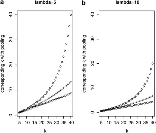
Sequencing effort k* of a pooling experiment to get allele frequency estimates with the same accuracy as in a standard experimental setup where k individuals are sequenced separately. (“o”, pool size n = 50; “+”, n = 100; “x”, n = 500.)

Open in new tab Download slide

In genome-wide association studies, the association between allele frequencies and traits (diseases) is investigated. A possible approach is to test whether alleles have different frequencies in two pools that differ with respect to the trait of interest (see Sham et al. 2002). Since the ratio of variances (10) does not depend on the allele frequencies in the subpopulations, the standard deviation entering the test statistic will differ by the square root of (10) between a pooling and a classical experimental setup. If the square root of (10) is

\(\frac{1}{2}\)

(say), the shift of the expected value of the test statistic under the alternative will be twice as large in a pooling experiment: Overall pooling will be the more powerful approach, whenever the variance ratio is smaller than one [see (10)]. It should be noted, however, that the variance of the pooling experiment will become larger if individuals contribute unequal amounts of probe material. This issue is addressed in the last paragraph of this section.

Estimating population genetic parameters:

We now compare the estimation of the scaled mutation parameter using Watterson's θ and Tajima's π under our two experimental setups. For this purpose, we simulated 100 samples each consisting of 500 sequences under neutrality with mutation parameter θ = 10, using the ms software (Hudson 2002). For separate sequencing, we took random subsamples of size k = 10 from each sample, thus simulating separate sequencing of 10 individuals each with an expected number λ of reads. With pooling, we took samples of size n of the 500 simulated sequences. From this pool, reads were taken independently for each locus l by making a random number of draws M_l with replacement. The quantities M_l were chosen according to a Poisson distribution with expected value kλ. Figure 4 illustrates that there can be considerable bias when Watterson's θ and Tajima's are used naively. For Tajima's π, we therefore used the bias correction (14) for individual loci and added the estimates across loci using (15). For Watterson's θ, the bias was corrected using Equation 18 for each locus.

Neglecting sequencing errors for the moment, it turns out that the pooling approach with bias correction leads to more accurate estimates of θ and π, provided that the size of the pool is large enough. For small pools, multiple reads of the same chromosome become more common, which affects the accuracy of the estimates negatively (Figure 4).

Figure 4.—

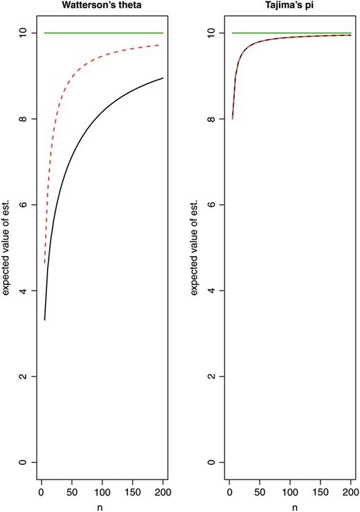
Expected value of the estimates obtained from pooled samples depending on the pool size n: Watterson's θ and Tajima's π. True value θ = 10 (green line). There is a considerable bias, if n is small compared to kλ, illustrating the need to use a bias correction with the estimates. Solid black line, λ = 30; red dashed line, λ = 5. (For Tajima's π, the bias does not depend on λ.)

Open in new tab Download slide

We now investigate the pooling approach when including a protection against sequencing errors by removing all segregating sites where the minor allele that has frequency x satisfies x = 1 or alternatively x ≤ 2. Again, the normalizing constants have been adapted to avoid bias. Let b denote the minimum required minor allele frequency.

Figure 5 shows the relative advantage of pooling conditional on different minimum minor allele frequencies. Pooling still leads to a decreased variance under neutrality as long as the pool size is large enough. Not unexpectedly, the reduction in variance is now somewhat smaller for Watterson's

\(\mathrm{{\hat{{\theta}}}}_{\mathrm{W}}^{(b){\ast}}\)

⁠. The increase in the variance of Tajima's

\(\mathrm{{\hat{{\theta}}}}_{\mathrm{{\pi}}}^{(b){\ast}}\)

is much smaller, since frequency 1 minor alleles receive a low weight in the calculation of π.

Figure 5.—

Variance ratio (Var_pooled/Var_standard) of the bias-corrected version of Watterson's θ and Tajima's π depending on the pool size n. We consider pooling both without [minor allele frequency (MAF) ≥ 1] and with a protection (MAF ≥ 2, MAF ≥ 3) against sequencing errors. (Only segregating sites with MAF above the stated threshold are included.) The horizontal green line denotes the break-even ratio of 1, where both the pooled and the classical experiment leads to estimates with equal variances. Pooling always performs better, as soon as the size of the pool exceeds the number of separately sequenced individuals. Solid black line, λ = 30; red dashed line, λ = 5. Standard setup is shown with k = 10 individuals sequenced separately.

Open in new tab Download slide

Unequal amounts of probe material:

One obvious source of error in the pooling approach is the heterogeneity in DNA amounts due to measurement errors. In experiments that rely on PCR amplification, the heterogeneity can be expected to be particularly strong.

Individuals for which a larger DNA amount has been included in the DNA pool will be overrepresented, which potentially causes a change in allele frequency estimates. This affects the bias and the variance also for our considered population genetic summary statistics.

To investigate the sensitivity of population genetic estimates based on pooling experiments, we simulated a scenario involving unequal amounts of probe material. We set the expected amount of probe material to one and allowed for log-normally distributed multiplicative deviations from this expected value. More specifically, the deviation factors were chosen independently for each individual contributing to the pool according to exp(X_i), where X_i (1 ≤ i ≤ n) are normal N(0, log(scale)) random variables. Thus the median amount of probe material is always equal to 1. If the deviation factor has a value of exp(X_i) = 1.5, this means that the respective individual will have a 50% higher chance of being sequenced than another with a factor of exp(X_i) = 1. Similarly, a value of 0.8 means a 20% decreased chance of being read.

As our first scenario (scale = 2), slightly more than 30% of all individuals differed at least twofold from the median. In other words, for a pool of size n = 100, the most abundant individual contributed ∼16 times the probe material of the least abundant individual. We also simulated a more extreme scenario (scale = 8), where ∼30% of the individuals differed at least eightfold from the median. As further parameters we chose λ = 30, k = 10, n ∈ [5, 200].

As the amount of heterogeneity in the sample will usually be unknown, we applied the same bias correction as for equal amounts of probe material. We measured the deviation from the true θ by the mean squared error, as this accounts for bias and variance.

Figure 6 displays the effect of heterogeneity in probe material on the bias and the variance of Tajima's π and Watterson's θ. Although both bias and variance change noticeably for higher levels of heterogeneity, these effects cancel out to a large extent. Thus the overall performance measured in terms of the mean squared error,

\[\mathrm{MSE}{=}\mathrm{Bias}^{2}{+}\mathrm{Var},\]

(20)

changes only marginally even for a large level of heterogeneity (scale = 8); see Figure 7. This effect can be explained by shrinkage that leads to improved estimates of the mutation parameter θ by permitting for some bias (Futschik and Gach 2008).

Figure 6.—

Bias (solid lines) and variance (dashed lines) of Watterson's θ and Tajima's π depending on the extent of heterogeneity in probe material. Black lines, moderate heterogeneity (scale = 2); red lines, high heterogeneity (scale = 8). In the top row bias and standard deviations are plotted for the population genetic estimates. The bottom row contains the squared bias and the variance that add up to the mean squared error. [Further parameters, λ = 30, k = 10; log-normal parameters, μ = 0, σ = log(scale).]

Open in new tab Download slide

Figure 7.—

Mean squared error ratio (MSE_pooled/MSE_standard) of Watterson's θ and Tajima's π depending on the pool size n and for λ = 30. Solid black line, the same amount of probe material is available for all individuals; red dashed line, the amount of probe material differs from individual to individual according to log-normal factors. For the top two panels, both curves are nearly identical. The median factor is always 1, and with a scale of 2, ∼32% of all probes deviate by a factor of more than the value given by scale. For a scale value of 2 (for instance), 16% of probes involve more than double the median probe amount, and another 16% contain less than one-half the median amount. [Log-normal parameters: μ = 0, σ = log(scale), scale ∈ {2, 8}.]

Open in new tab Download slide

Heterogeneity in probe material also affects the accuracy of the estimated allele frequencies, as the variance of the estimator based on a pooled sample becomes larger. However, this effect can be kept small, by choosing a pool of a large enough size. This is illustrated in Figure 8, where it can be seen that pooling leads for large enough pool sizes eventually to smaller variances even for a high level of heterogeneity in probe material (scale = 8).

Figure 8.—

Variance ratios (Var_pooled/Var_standard) when estimating allele frequencies in the case where the amount of probe material also differs from individual to individual according to log-normal factors. The median factor is always 1, and with a scale of s, ∼32% of all probes deviate by a factor of more than s. For the scale value s = 2 (for instance) 16% of probes involve more than double the median probe amount, and another 16% contain less than one-half the median amount. Ratios <1 indicate that pooling leads to estimates with a smaller variance. Individual sequencing is carried out for 10 individuals with an expected coverage of λ = 10. Scales: s = 2 (red dashed line), s = 4 (green dotted line), s = 8 (blue dashed-dotted line). [Log-normal parameters: μ = 0, σ = log(scale), scale ∈ {2, 4, 8}.]

Open in new tab Download slide

DISCUSSION

Over the past decades we have been witnessing a continuous turnover of molecular markers used in genetic research. To a large extent this turnover has been driven by the advances in molecular biology and technology. With the arrival of the second-generation sequencing technologies, this race is about to come to an end—rather than relying on a more or less representative fraction of the genome, it has come into reach to have full genomic sequences available for multiple individuals.

With further technological advances, it is anticipated that it will become possible to sequence individual genomes at a cost that allows even small laboratories to perform population analyses on a genome scale. Currently, this is not possible as the costs are still too high. In this study, we showed that sequencing pools of individuals provides an excellent alternative that permits genome-wide polymorphism surveys at very moderate costs.

This is the first report systematically exploring the parameter range for which DNA pooling provides an advantage compared to individual genome sequencing.

Our result that NGS of DNA pools often provides a reliable and cost-effective means for genome-wide allele frequency estimates is supported by some recent studies using NGS to analyze DNA pools of selected genomic regions. Van Tassell et al. (2008) sequenced a complexity-reduced DNA pool using the Illumina Genome Analyzer. For a subset of the identified SNPs, they compared the allele frequency estimates from the Illumina sequencing to those obtained by genotyping the same individuals. Despite that SNP frequency estimates were undoubtedly affected by a substantial assignment error (Palmieri and Schlötterer 2009) due to the short reads and the complexity-reducing procedure, Van Tassell et al. (2008) observed a correlation of 0.67 between the two methods. Hence, there is very little doubt that NGS is an effective tool to provide accurate genome-wide allele frequency estimates from DNA pools.

We anticipate that the analysis of DNA pools will provide a wide range of applications. In population genetics, it will be possible to compare patterns of differentiation on a genomic scale. Thus, patterns of local adaptation and heterogeneity in gene flow among different genomic regions can be identified. Also, for association mapping DNA pools are very powerful (Sham et al. 2002). In contrast to SNP arrays, however, resequencing of DNA pools will always include the causative SNP and thus provide a higher statistical power. Our study provides the basis for an adequate experimental design of future pooling experiments.

Footnotes

Communicating editor: D. Begun

Acknowledgements

We especially thank C. Kosiol, N. de Maio, and R. Kofler for helpful comments on earlier versions of the manuscript. We are grateful to A. Vasemägi and J. Wolf for general discussions about pooling for NGS, and we also thank the reviewers for helpful comments. This work was supported by a Wiener Wissenschafts-, Forschungs- und Technologiefonds grant to A.F. and C.S. as well as by Fonds zur Förderung der wissenschaftlichen Forschung grants (P 19832-B11 and L403-B11) awarded to C.S.

References

Achaz, G.,

2008

Testing for neutrality in samples with sequencing errors.

Genetics

179

:

1409

–1424.

Crossref

PubMed

Durrett, R.,

2008

Probabiliy Models for DNA Sequence Evolution. Springer, New York.

Eberle, M., and L. Kruglyak,

2000

An analysis of strategies for discovery of single-nucleotide polymorphisms.

Genet. Epidemiol.

19

:

S29

–S35.

Crossref

PubMed

Erlich, Y., K. Chang, A. Gordon, R. Ronen, O. Navon et al.,

2009

DNA sudoku—harnessing high-throughput sequencing for multiplexed specimen analysis.

Genome Res.

19

:

1243

–1253.

Crossref

PubMed

Futschik, A., and F. Gach,

2008

On the inadmissibility of Watterson's estimate.

Theor. Popul. Biol.

73

:

212

–221.

Crossref

PubMed

Holt, K., Y. Teo, H. Li, S. Nair, G. Dougan et al.,

2009

Detecting SNPs and estimating allele frequencies in clonal bacterial populations by sequencing pooled DNA.

Bioinformatics

25

:

2074

–2075.

Crossref

PubMed

Hudson, R. R.,

2002

Generating samples under a Wright-Fisher neutral model of genetic variation.

Bioinformatics

18

:

337

–338.

Crossref

PubMed

Jiang, R., S. Tavaré and P. Marjoram,

2009

Population genetic inference from resequencing data.

Genetics

181

:

187

–197.

Crossref

PubMed

Knudsen, B., and M. M. Miyamoto,

2009

Accurate and fast methods to estimate the population mutation rate from error prone sequences.

BMC Bioinformatics

10

:

247

.

Crossref

PubMed

Lynch, M.,

2008

Estimation of nucleotide diversity, disequilibrium coefficients, and mutation rates from high-coverage genome-sequencing projects.

Mol. Biol. Evol.

25

:

2421

–2431.

Crossref

PubMed

Lynch, M.,

2009

Estimation of allele frequencies from high-coverage genome-sequencing projects.

Genetics

182

:

295

–301.

Crossref

PubMed

Palmieri, N., and C. Schlötterer,

2009

Mapping accuracy of short reads from massively parallel sequencing and the implications for quantitative expression profiling.

PloS One

4

:

e6323

.

Crossref

PubMed

Sham, P., J. S. Bader, I. Craig, M. O'Donovan and M. Owen,

2002

DNA pooling: a tool for large-scale association studies.

Nat. Rev. Genet.

3

:

862

–871.

Crossref

PubMed

Van Tassell, C. P., T. P. Smith, L. K. Matukumalli, J. F. Taylor, R. D. Schnabel et al.,

2008

SNP discovery and allele frequency estimation by deep sequencing of reduced representation libraries. Nat.

Methods

5

:

247

–252.

This article is published and distributed under the terms of the Oxford University Press, Standard Journals Publication Model (https://dbpia.nl.go.kr/journals/pages/open_access/funder_policies/chorus/standard_publication_model)

Download all slides

Month:	Total Views:
January 2021	5
February 2021	19
March 2021	39
April 2021	50
May 2021	36
June 2021	19
July 2021	33
August 2021	30
September 2021	29
October 2021	34
November 2021	38
December 2021	21
January 2022	31
February 2022	42
March 2022	34
April 2022	45
May 2022	55
June 2022	19
July 2022	49
August 2022	48
September 2022	48
October 2022	36
November 2022	38
December 2022	23
January 2023	45
February 2023	29
March 2023	71
April 2023	50
May 2023	25
June 2023	49
July 2023	39
August 2023	28
September 2023	17
October 2023	70
November 2023	40
December 2023	43
January 2024	40
February 2024	47
March 2024	69
April 2024	31
May 2024	36
June 2024	43
July 2024	48
August 2024	38
September 2024	32
October 2024	54
November 2024	74
December 2024	29
January 2025	26
February 2025	34
March 2025	42
April 2025	35
May 2025	14

Article Contents

The Next Generation of Molecular Markers From Massively Parallel Sequencing of Pooled DNA Samples

Abstract

METHODS

SNP detection:

Separate sequencing of individuals:

Pooling experiment:

Allele frequency inference:

Estimating population genetic parameters:

RESULTS

SNP detection:

Allele frequency inference:

Estimating population genetic parameters:

Unequal amounts of probe material:

DISCUSSION

Footnotes

Acknowledgements

References

Citations

Views

Altmetric

Email alerts

See also

Companion Article

Citing articles via

Latest

Most Read

Most Cited

Article Contents

The Next Generation of Molecular Markers From Massively Parallel Sequencing of Pooled DNA Samples Free

Abstract

METHODS

SNP detection:

Separate sequencing of individuals:

Pooling experiment:

Allele frequency inference:

Estimating population genetic parameters:

RESULTS

SNP detection:

Allele frequency inference:

Estimating population genetic parameters:

Unequal amounts of probe material:

DISCUSSION

Footnotes

Acknowledgements

References

Citations

Views

Altmetric

Email alerts

See also

Companion Article

Citing articles via

Latest

Most Read

Most Cited

This Feature Is Available To Subscribers Only

The Next Generation of Molecular Markers From Massively Parallel Sequencing of Pooled DNA Samples