


Abstract
Loci involved in local adaptation can potentially be identified by an unusual correlation between allele frequencies and important ecological variables or by extreme allele frequency differences between geographic regions. However, such comparisons are complicated by differences in sample sizes and the neutral correlation of allele frequencies across populations due to shared history and gene flow. To overcome these difficulties, we have developed a Bayesian method that estimates the empirical pattern of covariance in allele frequencies between populations from a set of markers and then uses this as a null model for a test at individual SNPs. In our model the sample frequencies of an allele across populations are drawn from a set of underlying population frequencies; a transform of these population frequencies is assumed to follow a multivariate normal distribution. We first estimate the covariance matrix of this multivariate normal across loci using a Monte Carlo Markov chain. At each SNP, we then provide a measure of the support, a Bayes factor, for a model where an environmental variable has a linear effect on the transformed allele frequencies compared to a model given by the covariance matrix alone. This test is shown through power simulations to outperform existing correlation tests. We also demonstrate that our method can be used to identify SNPs with unusually large allele frequency differentiation and offers a powerful alternative to tests based on pairwise or global FST. Software is available at http://www.eve.ucdavis.edu/gmcoop/.
LOCAL adaptation to divergent environments can lead to dramatic differences in average phenotype between populations of the same species. Such variation offers particularly compelling evidence of natural selection when it is correlated with variation in environmental factors over multiple independent geographic regions and/or species. For example, in warm-blooded species, individuals at higher latitudes tend to be smaller than those found at the equator (Bergmann 1847; Allen 1877) and birds in humid climates tend to be darker in pigmentation than those in drier habitats (Gloger 1833). There are many other examples of phenotypic adaptations to local environments, including cyptic pigmentation in deer mice (Sumner 1929; Mullen and Hoekstra 2008), body size and pigmentation gradients in Drosophila (e.g., Coyne and Beecham 1987; Hueyet al. 2000; Pool and Aquadro 2007), skin pigmentation clines in humans (Relethford 1997), and toxic soil resistance in plants (Jain and Bradshaw 1966). Such patterns were among the earliest types of evidence used to demonstrate the action of local adaptation as a force driving phenotypic differences between populations within a species (e.g., Huxley 1939; Mayr 1942).
Correlations between phenotype and environment may be mirrored at the level of individual genetic polymorphisms, where at some loci, allele frequencies strongly differentiate populations that live in different environments. Such correlations can arise when selection pressures exerted by the environmental variable are sufficiently divergent between geographic locations, such that differences in allele frequency can be maintained in the face of gene flow (e.g., Haldane 1948; Slatkin 1973; Nagylaki 1975; Lenormand 2002). The study of geographic patterns of genetic variation has a long history, with some of the earliest work on genetic polymorphism being the study of clines in the frequency of cytologically visible inversion polymorphisms (Dobzhansky 1948). Other examples include loci involved in adaptations to high altitude (Storzet al. 2007; McCrackenet al. 2009), pigmentation (Hoekstraet al. 2004), and life-history changes (Schmidtet al. 2008). One particularly impressive example of adaptive response to selection is provided by the ADH locus in Drosophila melanogaster, alleles of which show a strong gradient with latitude (Berry and Kreitman 1993). It has been observed that the ADH cline is quickly reestablished after the introduction of the species onto different continents and that it responds quickly to climate change (Uminaet al. 2005).
The advent of genome-wide data sets with individuals from many populations, across a wide geographic range (e.g., Nordborget al. 2005; Jakobssonet al. 2008; Liet al. 2008; Autonet al. 2009), allows investigators to obtain a systematic view of the processes shaping local adaptation and to gain valuable insights into the genetic and ecological basis of adaptation and speciation. It can also provide support for adaptive explanations for phenotypic variation, for example, suggesting an impact of selection on variation that is linked to human metabolic diseases (Thompsonet al. 2004; Younget al. 2005; Hancocket al. 2008, 2010; Pickrellet al. 2009).
Some of the earliest tests of selection on genetic markers were based on identifying loci that showed extreme allele frequency differences among populations (Cavalli-Sforza 1966; Lewontin and Krakauer 1973), using statistics such as FST, and there are now a range of methods predicated on this idea (e.g., Beaumont and Balding 2004; Foll and Gaggiotti 2008). Our goal here differs, as we seek to identify loci where the allele frequencies show unusually strong correlations with one or more environmental variables. Such loci may be under selection driven by those environmental factors or correlated selection pressures. However, this goal is complicated by the fact that allele frequencies are typically correlated among closely related populations; since such populations tend to be geographically proximate they often share environmental variables (see Novembre and DiRienzo 2009 for a recent discussion). This means that neighboring populations can rarely be treated as independent observations. Thus, a naive test of correlation between population frequency and an environmental variable will often have a high false positive rate. This situation is somewhat analogous to the reduced number of independent contrasts when comparing traits across species due to the shared phylogeny (Felsenstein 1985). The nonindependence of populations is also known to be an issue when using FST as a summary statistic to identify selected loci (Robertson 1975; Excoffieret al. 2009).
To illustrate the problem, Figure 1 shows the allele frequencies of a SNP in a series of 52 human populations, as a function of the distance of each population from the equator (Figure 1 is redrawn from a similar plot in Thompsonet al. 2004). The SNP is AGT M235T and the allele that increases in frequency with latitude is known to reduce sodium retention (Liftonet al. 1993), which may have been selectively favored in cooler northern climes. However, as is apparent in Figure 1, populations cluster by broad geographic region for both allele frequency and distance from the equator. Thus, the correlation between allele frequency and environmental variable is clearly supported by far fewer independent observations than the 52 points plotted in Figure 1. Moreover, it is not clear how much of the variation in allele frequency in Figure 1 is due to sampling error in some of the smaller samples or genetic drift. For example, are the low allele frequencies in Oceania—which support an environmental correlation—simply due to sampling error or genetic drift?
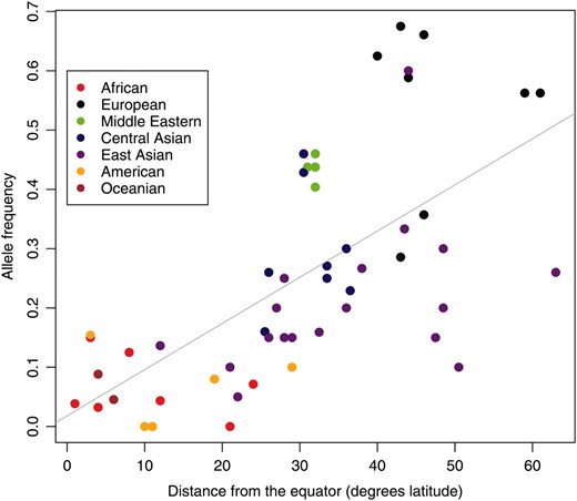
The distance from the equator for each of 52 human populations, plotted against sample allele frequencies for the SNP AGT M235T in each population. The points are colored according to the geographic region each population belongs to, following region definitions of Rosenberget al. (2002). The data were generated using HGDP samples by Thompsonet al. (2004) and are replotted on the basis of a figure in that article.
In this article, we develop a model to overcome these difficulties by accounting for differences in sample sizes and for the null correlation of allele frequencies across populations when testing for correlation between an environmental variable and allele frequencies. To do this, we use a set of control loci to estimate a null model of how allele frequencies covary across populations. We can then test whether the correlation seen between the allele frequencies at a marker of interest and an environmental variable is greater than expected given this null model. We concentrate on markers such as SNPs that are codominant and usually biallelic, but we note in the discussion how the model can be extended to other types of markers. The method developed here can be applied to continuous or discrete environmental variables. We demonstrate the method by applying it to genome-wide SNP data from humans. Elsewhere we have applied this method to human genome-wide SNP data, for a range of environmental and ecological variables (Hancocket al. 2008, 2010).
METHODS
We develop a model for the joint allele frequencies across populations. One way to do so would be to use a fully explicit model of demographic history, but such models are very difficult to parameterize and to fit for so many populations. Instead, we intentionally avoid using an explicit model of the historical relationships between populations and opt for a flexible, less model-based parameterization. Under our null model, the population allele frequency in each population may deviate away from an ancestral (or global) allele frequency due to genetic drift. Populations covary in the deviation that they take, allowing some populations to be more closely related genetically to each other due to the effects of shared population history or gene flow. Thus, our null model is specified by the covariance structure of allele frequencies across populations. To estimate this covariance structure, we assume that a transform of the population frequency of an allele across populations has a multivariate normal distribution. We estimate the covariance matrix of this normal distribution using our control SNPs. This provides the null model that we use to assess the correlation between the environmental variable and allele frequencies at a SNP of interest.
Null model:
Suppose that L unlinked SNPs have been typed in K populations. First we estimate the null model using all L of these markers; if the number of markers is very large, then to improve computational speed we may estimate the null model using a large random subset L of all the markers typed. (As discussed below, we find that the null model parameters estimated from different subsets of the data are highly consistent, provided that L is large enough.) In some applications, the markers that we are interested in testing for environmental correlations may be among the L (since we expect that a small fraction of selected loci will have little impact on the parameter estimates for the null model). Alternatively, the L may represent a set of well-matched control markers (see Hancocket al. 2008, 2010, for discussion).
The data at locus l consist of the number of times we see alleles 1 and 2, respectively, in each of the k populations. (The two alleles are labeled arbitrarily.) Then let nl = {n1l, … ,nKl} be the observed counts of allele 1 and ml = {m1l, · · · , mKl} be the counts of allele 2, in populations
We aim to construct a model for the joint distribution of allele frequencies across the k populations. If these frequencies were not constrained to be between zero and one, it would be natural to model the population allele frequencies of a SNP across populations as being multivariate normal. To overcome the constrained nature of allele frequencies, we follow Nicholsonet al. (2002) by assuming that the population allele frequency in a subpopulation, xkl, is normally distributed around an ancestral allele frequency εl (0 < εl < 1), but that the densities of xkl above 1 and below 0 are replaced with point masses on 1 and 0, respectively. Further, we adopt the assumption of Nicholsonet al. (2002) that, for a particular subpopulation, the variance of this normal distribution is a product of a factor that is constant across loci multiplied by a locus-specific term: i.e., εl(1 − εl). This model was introduced to describe a pure drift model where the allele frequency within each population independently drifts from the ancestral allele frequency. The normal distribution was chosen because, when the frequency of an allele in the current generation is ε, the binomial sampling of the next generation can be approximated as the frequency in the next generation being ∼N(εl, εl(1 − εl)/(2Ne)) (in a population of effective size Ne). Thus, after τ generations of genetic drift, the distribution of allele frequency can be approximated as ∼N(y, Ckεl(1 − εl)), where Ck = τ/(2Ne) is shared across loci, for τ ≪ Ne (Nicholsonet al. 2002). The estimate Ck can also be viewed as a model-based population-specific estimate of FST, a relationship that holds for low values of Ck (Nicholsonet al. 2002), a point that we return to briefly in the discussion.
Our prior on the variance–covariance matrix Ω, P(Ω), is somewhat more complicated, as it must have weight only on the set of positive definite matrices (a requirement of the multivariate normal distribution). We use the inverse Wishart prior, which is often used as a prior on variance–covariance matrices because it is the conjugate prior for the variance–covariance matrix of a multivariate normal. The inverse Wishart is parameterized by W(ρR−1,ρ), where R is the prior K × K shape matrix and ρ (where ρ ≥ K) is a parameter controlling the strength of the prior (i.e., how much the posterior draws of the covariance matrix resemble the shape matrix). To make the prior as weak as possible we set ρ = K. We set R to be the identity matrix (i.e., Rij = 1 if i = j, and 0 otherwise), but investigate the effect of this choice of prior later.
Alternative model:
We note that while this model predicts a linear relationship between θl and Y, this does not necessarily imply a linear relationship between the population allele frequencies xl and Y due to the boundaries for the population allele frequency at 0 and 1. Note that β and Y could also be multivariate, allowing combinations of climate variables to be investigated. However, the allele frequencies at any one locus are intrinsic noisy; thus there is limited information about even a single climate variable correlation and so we refrain from implementing this multivariate option.
Assessing significance:
Various aspects of population history are likely to violate the simple assumptions of our model; therefore the addition of the linear dependence on an environmental variable might improve the fit to the frequencies of even neutral alleles. Indeed, when investigating the performance of the method, on control sets of SNPs chosen to be neutral (e.g., Conradet al. 2006; Hancocket al. 2008), we found that the distribution of Bayes factors differed dramatically between environmental variables. This variation in the distribution of Bayes factors, across environmental variables, was not seen in data sets simulated using the matrix estimated from the Human Genome Diversity Project (HGDP) data, suggesting that it represents a feature of the data (results not shown). Thus, a large Bayes factor supporting the alternative model may not be strong evidence that the SNP has been the target of selection. A robust way to overcome this problem is to apply the method to all of the control SNPs and build an “empirical distribution” of Bayes factors from the control SNPs. The Bayes factor for the SNP of interest (for a given environmental variable) can then be compared to this distribution to judge its significance (Hancocket al. 2008, 2010). For applications of the method we recommend that these empirical distributions are constructed separately for bins of mean global allele frequency and ascertainment scheme; this will control for features of the data not well captured by the model. We direct interested readers to Hancocket al. (2010), where these recommendations have been implemented in a genome-wide scan for adaptive alleles.
RESULTS
To explore our method, we initially applied our method to the genotype data gathered by Conradet al. (2006) for 927 individuals from the 52 human populations of the HGDP panel. These populations represent a reasonable sampling from around the world, although there are some notable gaps in the sampling. Conradet al. (2006) typed 2333 SNPs in 32 autosomal regions to study patterns of linkage disequilibrium. Although the SNPs within each region are in partial linkage disequilibrium, and thus violate our assumption of independence between SNPs, parameter estimates of the model should not be biased as a result (although this violation may lead to overconfident parameter estimates). Consistent with this, we get very similar results if we run the analysis on subsets of the genomic regions (results not shown). We first estimated the 52 × 52 variance–covariance matrix of the HGDP populations. We show a single draw from the posterior of the covariance matrix in Figure 2A and the correlation matrix computed from this matrix in Figure 2B. These matrices reveal the close genetic relationship of populations from the same geographic region, which is qualitatively similar to the groups identified by STRUCTURE for these data (Conradet al. 2006) and samples (Rosenberget al. 2002; Liet al. 2008). Also, the Uygur and Hazara populations are clearly picked out as showing higher covariance between the East Asian and Western Eurasia blocks than other populations within the blocks, consistent with the hypothesis that these populations result from recent admixture events between these broad geographic regions (Rosenberget al. 2002).
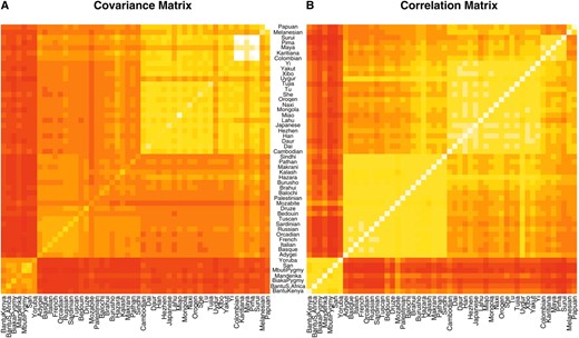
(A) A single draw from the posterior of the covariance matrix estimated for the HGDP SNPs of Conradet al. (2006). (B) The correlation matrix calculated from the covariance matrix shown in A. The matrices are displayed as heat maps with lighter colors corresponding to higher values. The rows and columns of these matrices have been arranged by broad geographic label.
The convergence of the MCMC to the posterior is relatively quick and dropping the first 5000 iterations was more than sufficient as a burn-in. Multiple independent runs with different starting positions quickly converged to similar matrices. Draws from the posterior showed relatively small fluctuations around the matrix displayed in Figure 2A, suggesting that the matrix is reliably estimated from this data set.
The posterior of the matrix estimated from these data is reasonably unaffected by the choice of prior of the covariance matrix. If instead of setting the shape matrix of the prior on the covariance matrix (R) to the identity matrix, we set it to specify a strong prior correlation (i.e., Rij = 1 if i = j and 0.99 for i ≠ j), there is no notable difference in the posterior estimate of the covariance matrix. For example, the Mantel matrix correlations between draws of the posterior matrix within a run are very similar to those observed between runs with different priors (results not shown). For applications to small numbers of markers and/or sample sizes, it may be advisable to use this prior shape matrix that reflects a strong correlation of allele frequencies between populations. This will encourage the method to combine information over small samples and will reduce the chance that populations with small samples will add noise to the test.
Power simulation:
Next we explored the power of our method to detect correlations between allele frequencies and environmental variables in the HGDP data. Simulating selection in a large number of populations under nonequilibrium models of history is challenging and unappealing, as it requires the arbitrary choice of many parameters. Instead we took an empirical approach and altered the sample frequency of the SNPs in the Conradet al. (2006) HGDP panel by adding a linear effect of the environment variable. If the current sample frequency of an allele in population k is Xk = nk/(nk + mk), then our new frequency is
We then calculated the Bayes factor to assess support for a correlation between Y and the modified SNP frequencies. For comparison, we also calculated the power of a number of other test statistics aimed at detecting the correlation between the environmental variable and the sample allele frequencies: Spearman's rank correlation ρ, the P-value from a linear regression model, and the P-value in a linear model obtained after first regressing out the first three principal components of the genetic data. We note that none of these three alternative methods offers a well-calibrated statistic; i.e., the P-values were not uniform under the null model (i.e., β = 0). Therefore, for these alternative methods and our Bayes factors we used the empirical distribution of a test statistic to correctly set the cutoff threshold for significance. To do this, we calculate the test statistic for all SNPs, applying no linear effect of the environmental variable (i.e., β = 0), and create an empirical distribution for each of these test statistics. We then find the 5% cutoff for this empirical distribution and any test statistic lower than this is declared significant at the 5% level. To explore the power of the various methods to detect an environmental correlation, we chose a geographic variable, i.e., latitude, and a climate variable, i.e., summer precipitation. Latitude was chosen because it has been used in a number of previous studies (e.g., Beckmanet al. 1994; Thompsonet al. 2004; Younget al. 2005; Hancocket al. 2008) and summer precipitation was chosen as an example where all methods should have good power because summer precipitation is relatively uncorrelated with genetic patterns (it has only mildly significant correlations with the first four principal components of the genetic data). In Figure 3, we show our power to detect a latitudinal effect on population allele frequency. As can be seen, the methods that account for the genetic structure of the populations outperform those that do not, and our method is the most powerful.
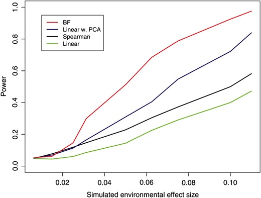
The power of various methods to detect a correlation between latitude and allele frequency.
When the environmental variable is reasonably uncorrelated with the major axes of variation in genetic data, the power of all of the methods improves, compared to the latitudinal results, as the “noise” caused by genetic relatedness between populations is less confounded with the signal that we are trying to detect. This can be seen clearly by comparing the power to detect an effect with summer precipitation (see Figure 4) to the latitudinal case, where all methods have lower power (note that both environmental variables have been standardized and so the average change in frequency is approximately the same in both cases). Also, the improvement in power of methods that account for genetic structure over those that do not is greatly reduced if the environmental variable is not strongly correlated with the principal axes of variation in the genetic data. For example, the power of Spearman's rank test to detect an effect of summer precipitation is comparable to that of the principal component method.
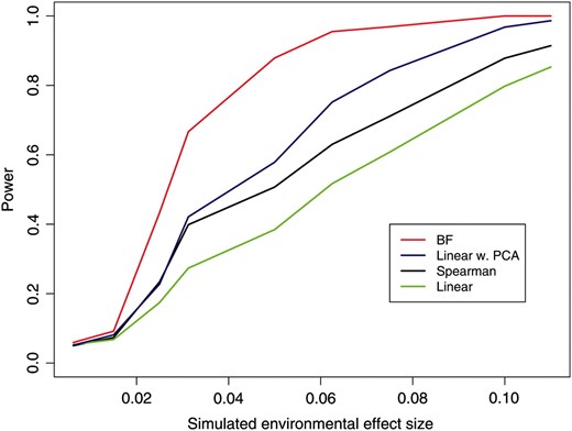
The power of various methods to detect a correlation between summer precipitation and allele frequency.
We also explored our power to detect a “continental” effect. To this end, we created an environmental variable Y, where Y = 1 for all European populations and Y = −1 for all non-European populations. We again calculated our power to detect such an effect using our estimated Bayes factor as a test statistic. For comparison, we also calculated the power to detect the effect using various FST-based measures between broad geographic areas: pairwise FST between the Middle East and Europe, pairwise FST between Central Asia and Europe, and a European population-specific measure of FST (these were all calculated according to Cockerham and Weir 1986 and Weir and Hill 2002). We also calculated a global FST using “continent”-level labels, but it performed very poorly, presumably because the changes in allele frequency were restricted to a subset of populations, and so was not included. The results of the power simulations are shown in Figure 5. Our method has higher power than the standard FST-based methods, perhaps because it effectively combines information from all of the pairwise comparisons in the data while accounting for the noise and covariance in each comparison (see also Excoffieret al. 2009 for discussion).
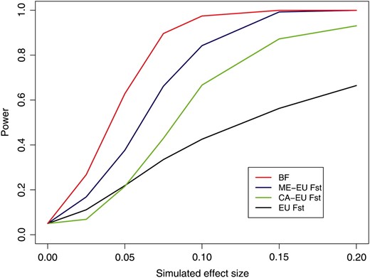
The power of various methods to detect a “European effect” on allele frequency.
Data application:
To demonstrate the utility of the method for genome-wide data, we applied the method to the 640,698 autosomal SNPs typed by Liet al. (2008) in the HGDP–CEPH. An expanded exploration of these data for a range of environmental variables is given in Hancocket al. (2010). Since the genotyped SNPs come from three different ascertainment panels (Eberleet al. 2007), we estimated three different covariance matrices, by sampling three different sets of 10,000 SNPs at random from the three different SNP sets. Draws from the posterior of the three covariance matrices estimated were qualitatively very similar to the example shown in Figure 2 and to each other and showed little variation within runs of the MCMC (results not shown).
We calculated the Bayes factors for all autosomal SNPs for a number of different continental effects, using the covariance matrix for each SNP that matched its ascertainment set. All of the calculated Bayes factors, along with the matrices used, are available for download at http://www.eve.ucdavis.edu/gmcoop/. In Figure 6, we show the Bayes factors for all autosomal SNPs for two of the effects tested: a European effect and a Western Eurasian effect (Europe, Middle East, and Central Asia). For example, for the European effect we set Y = 1 for all European populations and Y = −1 for all other populations and then standardize Y.
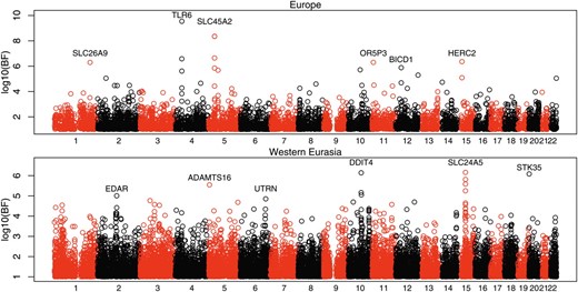
A plot of the log10 Bayes factor for each SNP along the human genome for (A) a European effect and (B) a western Eurasian effect. Bayes factors <1 are not plotted. The numbers on the x-axis indicate chromosome number, with SNPs on different chromosomes colored alternately in red and black. We list the name of the gene that is nearest to each of the six highest-ranking SNPs in each plot (considering only the peak SNP in each cluster of high Bayes factors).
Among our top hits for a European effect are previously identified hits at TLR6 (Toddet al. 2007; Pickrellet al. 2009), SLC45A2 (Nortonet al. 2007), and HERC2 (Sulemet al. 2007). Variants at these genes are known to be involved in immune response, skin pigmentation, and eye color, respectively. All of these alleles strongly differentiate the European populations from the closely related Middle Eastern and Central Asian populations. Instructively, SNPs in the Lactase gene are not among our top European effects, despite the selected allele being at high frequency within Europe and almost absent in the Middle East. This is likely due to the fact that the selected allele is also at high frequency in Central Asia (Bersaglieriet al. 2004) and in fact SNPs near the lactase gene have some of the largest Bayes factors for a joint Europe–Central Asian effect genome-wide.
Our top hit for a Western Eurasian effect (Figure 6) is the previously identified signal at SLC24A5 (Lamasonet al. 2005). Interestingly, EDAR is among our top hits for a Western Eurasian effect; this gene was previously identified by Sabetiet al. (2007) as the putative target of the strong selective sweep in East Asians (and is among the top Bayes factor signals for an East Asian–America effect). The Bayes factor signal in Western Eurasia hints that this genomic region might have undergone separate sweeps in Western Eurasia and East Asia. To explore the signal for a second sweep using haplotype patterns in this region, we calculated the empirical P-value for the XPEHH statistic (Sabetiet al. 2007), which compared haplotype homozygosity between two populations, for a window containing this gene (see Pickrellet al. 2009 for details). The empirical P-value was 0.029 in Europe, 0.046 in the Middle East, and 0.026 in Central Asia, suggesting evidence of a second sweep, although less strongly than the XP-EHH signal in East Asians for this region (empirical P-value of 0.0015).
DISCUSSION
In this article, we develop a flexible model for examining the correlation in allele frequencies across populations, parameterized by the covariance matrix. Our main goal was to use this estimated covariance matrix to perform a parametric test of the effect of an environmental or continental variable on the frequency of an allele at a SNP, while controlling for the correlation of allele frequencies across populations. Therefore, this model has strong similarities to generalized linear mixed models, where the environmental variable is a fixed effect and the covariance matrix governs the random effects. Thus, the approach is conceptually similar to the approaches introduced to map phenotypes across individuals in strongly structured populations; in these approaches a kinship matrix is used to account for differences in the background genetic relatedness (Yuet al. 2006; Kanget al. 2008). The proposed test results in a considerable improvement in power to estimate effects over methods widely used in the literature. This gain of power comes from the fact that the estimated covariance matrix informs the model as to how to weight the different populations.
For a single locus, the covariance matrix is proportional to the variance and covariance of allele frequencies around a common mean, where the constant of proportionality is the binomial variance εl(1 – εl). This means that the elements of the estimated matrix have a direct intepretation as a parametric estimate of the pairwise and population-specific FST. This interpretation holds only for relatively low levels of drift, as the boundaries at zero and one distort the relationship between the variance of the multivariate normal and FST for large levels of drift. Nicholsonet al. (2002) have an extensive discussion of this interpretation of the variance in the case where each population drifts independently from some shared ancestral population, and Weir and Hill (2002) and Samantaet al. (2009) discuss this connection for the maximum-likelihood estimator of the sample covariance matrix when levels of drift are low and sample sizes are large. The framework presented here thus provides a Bayesian model-based estimate of FST matrices discussed in Weir and Hill (2002). An alternative model-based formulation of population-specific FST is offered by the beta-binomial island-model framework (Balding and Nichols 1995; see also Balding 2003). This island-model framework considers populations at an equilibrium of mutation–migration–drift balance, as opposed to the nonequilibrium pure drift model of Nicholsonet al. (2002); the merits of these two approaches are discussed in Nicholsonet al. (2002), Baldinget al. (2002), and Balding (2003). The island-model framework has been extended to identify loci that have outlying allele frequencies with respect to particular populations (Beaumont and Balding, 2004; Bazinet al. 2010). Our aim here has been to develop a test of environmental selective gradients; thus while we have implemented this in the spirit of the pure-drift model of Nicholsonet al. (2002) our framework could be implemented into the island-model framework and would likely perform comparably [see also the discussion of choice of g() below].
The study of the pattern of the covariance of allele frequencies across populations has a long history as the covariance contains information about the history and levels of gene flow between populations (Cavalli-Sforzaet al. 1964; see also the review by Felsenstein 1982). It may be fruitful to adapt the Bayesian framework presented here to infer the historical relationships between the sampled populations. For example, the drift on different branches of a tree of populations could be approximated by normal deviations, which would allow rapid calculation of the branch lengths (see RoyChoudhuryet al. 2008 for a recent presentation of the problem). However, the pairwise covariance of allele frequencies across populations can be used only to learn about the average coalescent times within and between pairs of populations (Slatkin 1991) and so this approach could not be directly used to distinguish between isolation models and migration models (see McVean 2009, for discussion).
Here, we take a Bayesian approach that fully models the uncertainty in allele frequencies due to sampling. Thus, while we have discussed the model in terms of allele frequencies across population samples, it could be applied as an individual-based analysis where the genotype of each individual represents two draws from a unique “population.” This formulation may be useful when population labels are not known a priori. The current interest in principal component analysis (PCA), now almost exclusively based upon individual-level rather than population-level analyses, suggests that such applications would be useful, given that PCA is a decomposition of the covariance matrix (see McVean 2009, for discussion). Our method can also be extended to other marker types, e.g., for biallelic dominant markers, by using a different form from P(nl, ml | xl) (e.g., Falushet al. 2007). Likewise, the method could also be applied to data for pooled sample data or next-generation short-read sequencing data—once again by modifiying P(nl, ml | xl). We have also experimented with different transforms of the population frequencies [i.e., g()], e.g., a logit transform, and found that they gave very similar results, particularly in terms of the test of environmental variables (results not shown). Such transforms may be useful for applying the method to multiallelic systems such as microsatellites (e.g., Wasseret al. 2004).
We summarize the support for the model with an effect on an environmental variable compared to a model without a linear effect using a Bayes factor. In the application to the HGDP data, we ranked the SNPs by Bayes factor. A posterior predictive P-value (Rubin 1984) could be obtained by simulation from the posterior distribution of the null model, which would likely lead to a similar ranking. However, we have deliberately refrained from utilizing the method to make statements about the absolute “significance” of the correlation seen at specific SNPs, as we are somewhat skeptical about the fit of the null model even to data with no environmental dependence. Rather we suggest that careful comparison of the empirical distribution of test statistics (in our case Bayes factors) between a set of putatively selectively neutral control markers and candidate SNPs of interest is the most convincing way forward (Hancocket al. 2008). This can be accomplished in a genome-wide setting by genic to nongenic SNPs (assuming that nongenic sites are less likely to be functional) to judge the evidence for an enrichment of selection signals in the tails of a test statistic (Barreiroet al. 2008; Coopet al. 2009; Hancocket al. 2010). The empirical approach in turn has some serious drawbacks, the most obvious of which is deciding what statistical cutoff to use, as the choice of cutoff reflects one's prior beliefs of the prelevance of selection (Teshimaet al. 2006).
It is hard to predict in advance how often strong correlations between allele frequencies and environmental variables will form across a species range. However, it is likely that strong gene flow and the parallel mutation will both act to reduce the likelihood of strong correlations. If selection is not strongly divergent across a species range, i.e., the locally adaptated alleles are not selected against in other regions, then the selected allele will be spread across the species range by migration. Under these circumstances correlations may temporarily form but they may not persist for long, and these occurrences will also depend critically upon where the mutation arose and patterns of migration. [Even standard allele frequency differentiation-based methods may not identify a rapidly spreading sweep, and haplotype-based methods may be more informative (e.g., Voightet al. 2005).] In addition, the method will tend to detect only those loci where the environmental variable had a consistent effect on the frequency of a particular allele (due to either hitchhiking or the direct action of selection) and so may not detect regions of the genome where in different populations the same selection pressure has caused different haplotypes to go to fixation. Thus, if rates of gene flow are low across a species range compared to mutation rates toward the adaptive phenotype, then repeated evolution of a phenotype may occur by different genetic routes in different parts of the species range. For example, the genetic basis of pigmentation differs between geographic regions within a number of species (e.g., Hoekstra and Nachman 2003; Nortonet al. 2007; Edwardset al. 2010). Under these circumstances, the frequency of an allele will be correlated with an environmental variable only in parts of the species range. This suggests that it may be profitable to perform the analysis, including the estimation of the covariance matrix, separately in different geographic regions.
In closing, we note that while the method presented here is potentially very useful in identifying selected loci via their correlation with environmental variables, we caution against overintepreting the correlations (or lack of correlations) found. It is unlikely that causal selection pressures can be identified by such correlations as many environmental and ecological variables covary. Further, as outlined above, correlations may exist as a transient stage during the spread of a selected allele (even in the absence of a causal relationship). Thus we view this method as a powerful way of highlighting interesting loci and correlations that can be further explored by follow-up studies.
APPENDIX A: SAMPLING FROM THE POSTERIOR
We first describe how we calculate the posterior under the null model, and then we discuss the calculation of the Bayes factor in the next section. We wish to estimate the posterior of Ω integrating over our uncertainty in θ and ε. To do this, we use MCMC, where in each iteration of the MCMC algorithm we sequentially update the different parameters. Conditional on Ω and θl, we update εl at each locus using a standard Metropolis update, i.e., add a small normally distributed deviation to εl and accept the new εl if it falls within the range (0, 1), with a probability given by the ratio of the posteriors under the current and new value of ε.
We could use a similar proposal to update each θkl but since the θl are highly correlated over populations, we found that updating them individually results in a high rejection rate. Thus, we update the entire vector of transformed population frequencies (θl) simultaneously for a locus in a way that attempts to account for that correlation. Our proposal for the new transformed frequencies at a locus l,
APPENDIX B: EVALUATING THE BAYES FACTOR
Footnotes
Communicating editor: M. K. Uyenoyama
Acknowledgements
The authors thank Molly Przeworski, John Novembre, and members of the Di Rienzo, Pritchard, Przeworski, Stephens groups and the University of California at Davis Evolutionary Discussion Group for helpful discussions. We thank John Novembre, Molly Przeworski, Peter Ralph, and the reviewers for helpful comments on the manuscript. This work was supported by a Packard Foundation and Howard Hughes Medical Institute grant to J.K.P., by National Institutes of Health grants (DK56670 and GM79558) to A.D., and by a Sloan Foundation Fellowship to G.C.
References
Allen, J.,
Balding, D. J., A. D. Carothers, J. L. Marchini, L. R. Cardon, A. Vetta et al.,
Bergmann, C.,
Cavalli-Sforza, L.,
Cavalli-Sforza, L. L., I. Barrai and A. W. Edwards,
Cockerham, C., and B. Weir,
Coop, G., J. K. Pickrell, J. Novembre, S. Kudaravalli, J. Z. Li et al.,
Eberle, M., P. Ng, K. Kuhn, L. Zhou, D. Peiffer et al.,
Gloger, C. L.,
Hancock, A., D. B. Witonsky, E. Ehler, G. Alkorta-Aranburu, C. Beall, et al.,
Jain, S., and A. Bradshaw,
Lenormand, T.,
Lifton, R. I., D. Wamock, R. Acton, L. Harman and J-M. Lalouel,
Liu, J.,
Mayr, E.,
Nicholson, G., A. Smith, F. Jónsson, O. Gústafsson, K. Stefánsson et al.,
Norton, H., R. Kittles, E. Parra, P. McKeigue, X. Mao et al.,
Odell, P., and A. Feiveson,
Rubin, D. B.,
Schmidt, P. S., C. T. Zhu, J. Das, M. Batavia, L. Yang et al.,
Sumner, F.,
Voight, B., A. Adams, L. Frisse, Y. Qian, R. Hudson et al.,
Wasser, S. K., A. M. Shedlock, K. Comstock, E. A. Ostrander, B. Mutayoba et al.,
