Molecular Evolution in Small Steps under Prevailing Negative Selection: A Nearly Universal Rule of Codon Substitution Open Access

Abstract

Introduction

Since the time of Darwin, biologists have accepted that evolution proceeds in small steps. An obvious explanation is mutational input: Large changes require many mutations and each only makes an incremental contribution. Approaching the issue from the angle of natural selection, R.A. Fisher formalized the selectionists’ view of small-step evolution, known as Fisher’s Geometric Model (FGM) (Fisher 1930). FGM uses the metaphor of climbing the adaptive peak in a multidimensional landscape and suggests that small changes are more likely to be advantageous than large ones. At the molecular level, the neutral theory also posits small-step evolution, which can be summarized by two rules (Kimura 1983). 1) Functionally less important molecules evolve faster than functionally important ones. 2) Variants that are functionally similar to the wildtype are more likely to be substituted than dissimilar ones. The two rules are mainly about escaping negative selection but, when applied to positive selection, would converge with the FGM view. In this study, we focus on the second rule—coding-sequence evolution in small steps.

It is noteworthy that selectionists and neutralists appear to agree on small-step evolution, albeit with different emphases. In the neutralists’ view, negative selection tolerates small-step changes while FGM postulates that positive selection favors small-step improvements. Because negative and positive selections are distinct forces driving different processes, small-step evolution can be considered two models in one.

In this study, the step size of evolution is represented by amino acid (AA) differences (or distances) (Grantham 1974; Dayhoff et al. 1978; Miyata et al. 1979; Henikoff and Henikoff 1992; Kumar et al. 2009; Adzhubei et al. 2013). One approach to AA distances attempts to identify physicochemical properties of AAs that can best explain long-term substitution patterns. Earlier methods by Grantham (Grantham 1974) and Miyata (Miyata et al. 1979) and the more recent ones including SIFT (Kumar et al. 2009) and PolyPhen (Adzhubei et al. 2013) take this approach. The second approach attempts to identify substitution patterns directly from protein or DNA sequences and uses these evolutionary patterns as the proxy for AA distances. This second approach can be either AA based or codon based. For example, PAM (Dayhoff et al. 1978), LG (Le and Gascuel 2008), and BLOSUM (Henikoff and Henikoff 1992) are AA based, searching for long-term evolutionary patterns among the 190 (=20 × 19/2) pairwise comparisons. In contrast, the codon-based approach (Yang et al. 1998; Tang et al. 2004; Tang and Wu 2006) compares closely related species whose triplet codons differ by at most 1 bp. Among the 190 pairs, only 75 pairs can be exchanged by a 1-bp mutation. We shall take the codon-based approach to AA distances (Tang et al. 2004; Yang 2007).

The study, extending and revising the results of Tang et al. (2004) and Tang and Wu (2006), uses the tools developed therein (Tang et al. 2004; Tang and Wu 2006). The extensions are in three directions. First, in earlier studies, partial genomes are used. Given the partitions of AA changes into 75 kinds, the statistical resolution was barely adequate. These early releases of genomic data are also biased toward functionally important genes that bear distinct signatures of selection. Hence, whole-genome sequences obtained in the intervening years should be most useful. Second, it is important to densely sample within the same taxonomic rank (such as vertebrates, mammals, and primates) to test the consistency within the same phylum, class, or order. Third, and most important of all, previous studies did not separate the effects of positive and negative selection. For that reason, deviations from the general rule, potentially most informative about the working of the two opposing forces, have been ignored in previous studies.

With the AA distance as the step size of molecular evolution, the effects of negative and positive selection are separately analyzed in this and the companion report (Chen, He, et al. 2019). Here, we ask whether negative selection drives small-step evolution and whether there exist common rules at the codon level across a wide range of taxa.

Materials and Methods

Multiple Alignment Data

A multiple alignment file of 99 vertebrates with human for CDS regions was downloaded from the UCSC Genome Brower (http://hgdownload.cse.ucsc.edu/goldenPath/hg38/multiz100way/alignments/knownCanonical.exonNuc.fa.gz). We then selected seven representative pairs of species across vertebrates (supplementary table S1, Supplementary Material online). There were two pairs of species from the Primates order, one was from the family Hominidae (Homo sapiens and Pan troglodytes) and the other from the family Cercopithecidae (Macaca fascicularis and Callithrix jacchus). The other five pairs of species were from the order Rodentia (Mus musculus and Rattus norvegicus), the order Carnivora (Felis catus and Canis lupus familiaris), the order Artiodactyla (Bos taurus and Ovis aries), the class Aves (Geospiza fortis and Taeniopygia guttata), and the class Reptilia (Chelonia mydas and Chrysemys picta bellii). Additional technical details used here can also be found in Lin et al. (2018).

A multiple alignment file of 26 insects with Drosophilamelanogaster was also downloaded from the UCSC Genome Brower (http://hgdownload.cse.ucsc.edu/goldenPath/dm6/multiz27way/alignments/refGene.exonNuc.fa.gz). The genome sequences of D.melanogaster and Drosophilasimulans were then extracted from this file.

To correct for multiple hits for Ki/Ks, two closely related species of each pair were chosen from the same family. The alignment files were filtered using the following criteria: 1) Filter out genes in uncanonical scaffolds. 2) Use the corresponding AA multiple alignment file to remove noncoding genes. 3) Filter redundant transcripts generated by alternative splicing, based on a gene-transcript id conversion table downloaded from Ensembl biomart. 4) Genes aligned with too many gaps (more than 5%) were removed. 5) Genes shorter than 90 bp were removed. 6) Substitutions related to CpG sites in the Homo–Pan pair were masked because CpG-related substitutions account for more than 30% of total substitutions in this pair. Hence, we masked CpG-related substitutions (CG => TG, CG => CA were replaced with NG => NG and CN => CN, respectively) using gorilla as an outgroup (supplementary fig. S3 and supplementary text III, Supplementary Material online).

We first obtained protein and DNA sequences of Arabidopsis thaliana and Arabidopsis lyrata from the Phytozome database (Goodstein et al. 2012). We then extracted gene alignments using the PAL2NAL program (Suyama et al. 2006) with the mRNA sequences and the corresponding protein sequences for 1:1 orthologous pairs aligned by MUSCLE (Edgar 2004) using default parameters.

Ki/Ks Calculation

Here, $quv$ is the instantaneous rate from codon u to codon v. $κ$ is the transition/transversion rate ratio, $πv$ is the equilibrium frequency of codon v. $ωij$ is the nonsynonymous/synonymous rate ratio, where i (=aa_u) and j (=aa_v) are the two AAs involved. There are 75 $ωij$⁠, analogous to Ki/Ks (i = 1:75), of AA pairs whose codons differed by 1 bp. The method considering unequal substitution rate between different AAs has been summarized in Yang et al. (1998).

The controls in codeml are as follows:

1. codenFreq=0. Assuming individual codon frequencies are equal. There are four codon frequencies models in common use, including F-equal, F1×4, F3×4, and F61 (see p. 48 of Yang [2006]). We opt for the simplest F-equal and discuss the influence of codon frequency models to the estimated Ki/Ks (see supplementary figs. S5 and S6 and supplementary text VI and VII, Supplementary Material online).

2. Model=0. Assuming the $ωij$ is constant in different braches.

3. NSsites=0. Use the M0 (one ratio) model to estimate $ω$ for site models. Disregard the variation in $ω$ among sites.

4. aaDist=7. Divide AA substitutions into several groups and estimate their $ωij$ separately. The AA groups are summarized in a file called OmegaAA.dat. The setting in OmegaAA.dat is as following:

“−1

//end of file.

”

Here, putting −1 at the start of file, then the program will fit the “general model,” assigning an independent $ω$ for each one-step AA pairs, which corresponding 75 Ki/Ks. In the same time, the overall $ω$ (Ka/Ks) is also given in the output. See the supplementary table S4, Supplementary Material online, for the control file in codeml.

In the end, expected Ki/Ks values were calculated as E(Ki/Ks) = Ui × Ka/Ks in each pair of species.

Analysis of AA Distances

AA properties were extracted from table 2 of Gromiha et al. (1999). In total, 48 selected physicochemical, energetic, and conformational properties are given. The distances between AA pairs were defined by the differences in the raw values shown in their table 2. Various distance measures yielded similar results. The 48 distances of each AA pair were then scaled by the z-score method for the principal component analysis (PCA) and partial least square regression (PLSR) analysis. PCA and PLSR were performed using the R packages “factoextra” (Kassambara and Mundt 2017) and “pls” (Mevik et al. 2019), respectively. Exponential fitting was accomplished by using the function “nls” in R.

The Relationship between Ui and Ka/Ks

Orthologous genes for each paired species were divided into five categories with approximately equal number of nonsynonymous changes according to their Ka/Ks ranking. The Ka/Ks of each gene is calculated by codeml in PAML. Number of nonsynonymous changes of each gene is obtained by comparing the divergent sites between two species using our own codes. Genes with fewer than two substitutions were removed for further analysis. It is expected that Ka values increase when Ka/Ks values ascend and Ks values are stable in the five categories. This is true in most of cases. However, the top 20% group in Homo–Pan is an outlier, exhibiting a sharp decrease in Ks. This may due to the short divergence time between Homo and Pan. The Ks values of the five categories in the Homo–Pan comparison were replaced by genome-wide Ks. The Mus–Rattus comparison was removed in figure 5 because Ui values were deduced from the comparison between Mus–Rattus and a pair of yeast (Tang et al. 2004). The 95% confidence intervals for R² are obtained by bootstrapping.

Results

There have been a long series of studies that aim to group AA changes into classes, starting with Zuckerkandl and Pauling (1965), followed by Grantham (1974) and Miyata et al. (1979) (see supplementary text I, Supplementary Material online). In later studies, the classification is often along the line of radical versus conservative changes (Kr vs. Kc) (Smith 2003; Nabholz et al. 2013; Weber et al. 2014; Figuet et al. 2016). Because these classifications involve assigning AA changes into classes, the outcome has been reported to depend on the classification (Dagan et al. 2002; Hanada et al. 2007) (see supplementary text II, Supplementary Material online, for details). The 75 Ki/Ks classes, in contrast, involve no grouping as each pair of AA_i and AA_j is an elementary class. In the main text, we will show that 1) Ki/Ks’s are nearly universally correlated across taxa and 2) this high correlation reflects the physicochemical properties of AAs.

The Correlation among Ki/Ks’s across Taxa

We first calculate Ki/Ks between nine pairs of species using their whole-genome sequences (fig. 1A). Among them are one pair from plants (Arabidopsis), one pair of insects (Drosophila), and seven pairs of vertebrates with rodents (Mus–Rattus) representing the vertebrates. Each pair consists of two closely related species. Genome-wide Ka/Ks ratios of these nine pairs ranges from 0.12 to 0.27 (supplementary table S1, Supplementary Material online).

Fig. 1.

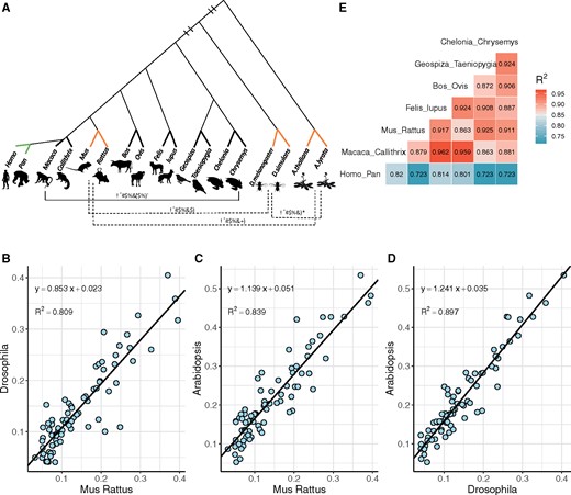
—Correlation of Ki/Ks values between different taxa. (A) Phylogenetic Tree of 9 representative species pairs (full names are shown in supplementary table S1, Supplementary Material online). R² values (pairwise correlation of Ki/Ks’s) range from 0.86 to 0.96 in 6 vertebrates (horizontal solid line), except for Homo–Pan pairs. Three species pairs, Rodent, Drosophila, and Arabidopsis (bold orange lines), are selected to show species pairs with long evolutionary distance. (B–D) Scatter plots of Ki/Ks between Rodent, Drosophila, and Arabidopsis. The solid black lines are linear regression lines and the legends on the top left are the regression formulas and their R². (E) Pairwise R² values of Ki/Ks among seven species pairs in vertebrates.

Open in new tabDownload slide

We then calculate the correlation in Ki/Ks between two pairs of distantly related taxa (fig. 1A). Pairwise correlations between Arabidopsis (A. thaliana vs. A. lyrata), Drosophila (D. melanogaster vs. D. simulans), and vertebrates (Mus vs. Rattus) are shown in figure 1B–D. The R² values are 0.81 (vertebrates vs. insects), 0.84 (vertebrates vs. plants), and 0.90 (insects vs. plants). Such strong correlations over a large phylogenetic span suggest that AA substitutions follow a nearly universal rule. Although Ki/Ks within each taxon may be very different, their relative magnitudes remain the same across all taxa. The correlations of figure 1B–D are close to the results obtained by Tang et al. (2004), thus permitting further analyses based on the earlier results.

We now examine the correlation in a dense phylogenetic framework by comparing species pairs of vertebrate classes or mammalian orders (fig. 1E). Although one might have expected the correlation to be even greater in the lower taxonomic rank, the observations of figure 1E suggest otherwise. In fact, the R² values are not strongly dependent on the phylogenetic distance. For example, R² in the Drosophila–Arabidopsis comparison is higher than many of the 21 comparisons between vertebrates. In particular, the AA substitutions between hominoids and other vertebrates often yield R² < 0.8. It seems plausible that similar forces work reiteratively from taxa to taxa, yielding a degree of consistency across the phylogeny.

The high correlation among Ki/Ks values permits a generalized (or universal) Ki/Ks measure as proposed before (Tang et al. 2004). Here, we shall briefly introduce the measure, referred to as Ui (Tang et al. 2004). It ranges between 0.25 and 2.5 for i = 1–75 and is the relative AA substitutions rate between 75 AAs. Ui is scaled such that the weighted mean is 1 across the 75 classes. For example, Ui = 2.5 represents substitutions rate for this AA is 2.5 times higher than average substitutions rate.

Ki/Ks in Relation to AA Distances

The high correlation across a large phylogenetic distance (fig. 1) suggests something as basic as physicochemical properties of AAs to be a major cause. It has been tantalizing to ask whether a small number of differences in these properties (AA distances, for short) might account for the evolution of protein sequences, thus reducing evolution to the simplest physical dimensions (Grantham 1974; Miyata et al. 1979).

We analyze 48 physicochemical, energetic, and conformational distances among AAs (fig. 2). As shown in supplementary table S2, Supplementary Material online, these properties are not all about each AA in isolation; many measurements (e.g., number of surrounding residues) depend on the context of protein sequences. These measurements are broadly depicted as “physicochemical,” as opposed to “functional.” We use Ui (i = 1, 75 [Tang et al. 2004]) to represent Ki/Ks across species primarily given that Ui is highly correlated with each species’ Ki/Ks (see fig. 4 below).

Fig. 2.

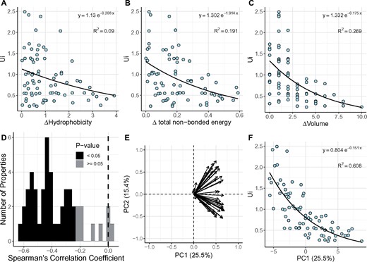
—The relationship between AA distances and Ui. Forty-eight physicochemical, energy, and conformational properties are used in the analysis. (A–C) Scatter plot of three selected AA distances against Ui, including hydrophobicity (A), total nonbounded energy (B), and volume (C). (D) Spearman’s correlation coefficients between 48 AA distances and Ui. Among those distances, 47 distances are negatively correlated with Ui, where 39 of them are significantly (black, P value < 0.05). (E) Contribution of 48 AA distances to the first 2 principal components. Properties cluster into two categories in the second principal component but are indistinguishable in the first principal component. (F) Scatter plot of the first principal component (PC1) against Ui.

Open in new tabDownload slide

Ui is fitted to each of the 48 AA distances via an exponential function (see Kimura 1983). Figure 2A–C shows regressions of Ui on AA distances of hydrophobicity, total nonbounded energy, and volume. Although hydrophobicity is generally thought to be an important attribute, the correlation is weak (R² = 0.09). Instead, the volume difference of AA explains more of the Ui variation with R² = 0.27, consistent with the prior conclusion on the relative importance of AA’s volume (Yang et al. 1998; Braun 2018). The spearman’s correlation coefficient for each AA distance is given in figure 2D, which shows that 47 of the 48 measures are negatively correlated with Ui and P < 0.05 is found for 39 of them (supplementary table S2, Supplementary Material online). Given the correlation with the evolutionary rate is nearly entirely negative for AA distances, the fitness effect is not likely to be narrowly distributed among a few AA distances.

Measures of these 48 AA properties are not randomly associated with the 75 AA pairs. Each pairwise comparison between the 48 measures is plotted for the 75 AA pairs to extract the correlation between these distances, designated Rd. The heatmap of all pairwise Rd’s is given in figure 3 where the inset shows one of the largest Rd’s between volume (property 4 of supplementary table S2, Supplementary Material online) and helical contact area (property 9). Rd = 0.94 for this pair indicates that these two distances probably reflect two very similar AA characters. Along the diagonal, some clustering can be discerned but the correlation is generally weak. There are nevertheless a few high-Rd pairs, shown as red squares along the diagonal. A subset of such red squares involving the top 13 AA distances of supplementary table S2, Supplementary Material online (P1–P13, with R > 0.5) are most relevant. They form six clusters which are identifiable based on their Rd’s—[P1, P11, P13], [P2, P8], P3, [P4, P7, P9, P10], [P5, P6], P12, where properties in brackets belong in the same cluster (see fig. 3 and supplementary table S2, Supplementary Material online). Thus, the 48 properties may behave like half the number of uncorrelated measures. It would then be more rigorous to do the PCA and PLSR analyses as done below.

Fig. 3.

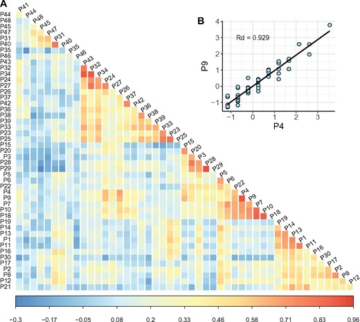
—The pairwise correlation between 48 amino acid distances. (A) The heatmap of pairwise correlation between different amino acid measurements. P1–P48 are the AA measurements listed in supplementary table S2, Supplementary Material online. The color bar represents the spearman’s correlation coefficients (Rd) between AA distances. (B) The inset figure above the diagonal shows the scatter plot (each dot being an AA pair) between the volume measurement (P4) and the helical contact area (P9) of each AA pair. This particular Rd is the second largest among all.

Open in new tabDownload slide

By the PCA, we show that PC1 explains about 61% of the Ui variation (fig. 2F). Figure 2E further shows that the contributions to PC1 are distributed broadly among the 48 measures with “helical contact area” in the lead, contributing about 4%. As PC1 accounts for only 25.5% of the variance of AA distances, the remaining variance should also be informative. This can be seen when the PLSR is used. In PLSR, the first component accounts for 60.1% of the Ui variation using 25.3% of the AA distance variance. The cumulative effect of the first five components accounts for 80% of the Ui variation, using <60% of the AA distance variance (supplementary fig. S1, Supplementary Material online). The results from PCA and PLSR are highly compatible.

The overall results of figures 2 and 3 suggest that the physicochemical properties of AAs, or any combinations of such properties, are not likely to be fully predictive of the evolutionary rates of protein sequences. In the early days, a small number of such properties were found to capture a moderate amount of evolutionary rate variation (Miyata [Miyata et al. 1979] and Grantham [Grantham 1974]). It is natural to be hopeful that additional AA properties coupled with extensive DNA sequencing might be fully predictive of the evolutionary rate of protein sequences. The study shows that the optimism cannot be realized. Nevertheless, it is still possible to predict the evolutionary rate of most taxa because the AA substitution patterns are generalizable across diverse taxonomic ranks. Figures 2 and 3 show that such general rules exist but they cannot be expressed in simple physicochemical terms. The evolutionary Ui measure remains the best predictor of the rate of AA substitutions when compared with Miyata and Grantham distances (see supplementary table S3 and supplementary text V, Supplementary Material online).

The General Rule for Small-Step Evolution Expressed as ΔU(i)

Given Ui, the AA distance of the ith pair can be more conveniently rescaled as Δ_U(i) =(U₁ − Ui)/(U₁ − U₇₅), which falls in the range of [0, 1] with Δ_U(1) = 0 for the closest pair, [Ser-Thr], and Δ_U(75) = 1 for the most distant pair, [Asp-Tyr].

The observed versus expected Ki/Ks for the nine pairs of species are shown in figure 4. The x axis is E(Ki/Ks), which can be written as [2.5 − 2.25 Δ_U(i)] × Ka/Ks (see the legend of figure 4 and supplementary table S1, Supplementary Material online, for details). There are three groups in this figure. The first group consists of three pairs of well-assembled genomes—Arabidopsis, Drosophila, and Rodents (fig. 4A, B, and G). All three taxa show R² > 0.9 between Obs(Ki/Ks) and E(Ki/Ks). It is notable that the R² improves significantly in Drosophila, rising from 0.706 to 0.904 in comparison with Tang et al. (2004), as the number of genes increases from 309 to 9,710. In the second group of five pairs of genomes of moderate quality (Fig. 4C-F, H), R² ranges between 0.77 and 0.85. Taking into account the room for improving their quality, we conclude that these species follow the nearly universal pattern of codon substitutions.

Fig. 4.

—Correlations of expected and observed Ki/Ks for nine species pairs. (A-I) Scatter plots between expected and observed Ki/Ks. Because Ui = U₁ − (U₁ − U₇₅) Δ_U(i), the x axis label can be written as E(Ki/Ks) = Ui × Ka/Ks = [2.5 − 2.25 Δ_U(i)] × Ka/Ks, which is a linear function of Δ_U(i). The boldface Ka/Ks, the genome-wide Ka/Ks, is the characteristic of each pair of species.

Open in new tabDownload slide

The third group consists of the one exceptional case of human–chimpanzee comparison (Fig. 4I), which yields an R² of 0.627, far lower than the rest. There may be several explanations for this unusually low R². Because codon substitutions involving CpG sites have been removed from consideration (see Materials and Methods), this obvious explanation is ruled out (see supplementary fig. S3 and supplementary text III, Supplementary Material online). The second explanation is the unusual selective pressure in the human lineage (Bustamante et al. 2005; Williamson et al. 2005; Subramanian 2011). However, because R² along the human, chimpanzee, and gorilla lineages is, respectively, 0.572, 0.638, and 0.646 (supplementary fig. S4 and supplementary text IV, Supplementary Material online), the human lineage does not stand out in this respect. Instead, we will show that hominoids as a group are unusual and many genes in their genomes have a high Ka/Ks ratio > 0.6.

The Rule of Small-Step Evolution Is Governed by Strong Negative Selection

Between each pair of species, we divide the genomes into five bins in the ascending order of Ka/Ks (see Materials and Methods). It seems intuitively true that R² would decrease as Ka/Ks increases. Imagine that, when Ka/Ks = 1 and under no negative selection, all observed Ki/Ks ratios would fluctuate around 1 and the correlation between the observed and expected Ki/Ks would be 0. Chen, He, et al. (2019) extend this intuition by an analytical model that incorporates negative selection of variable strength. A decrease in R² when Ka/Ks increases is confirmed by the model (see their fig. 1C).

The R² value (i.e., between Obs(Ki/Ks) versus E(Ki/Ks)) of each bin is plotted against the Ka/Ks value of that bin (fig. 5). There are two decreasing trends. First, R² is generally >0.6 for gene groups with Ka/Ks < 0.4. The drop in R² become steeper as Ka/Ks gets larger than 0.4. This important trend appears to escape notice in Tang et al. (2004). Second, the human–chimpanzee comparison follows the same pattern but generally at a lower level. Two opposing forces drive the trend of figure 5 with increasing Ka/Ks: weaker negative selection and/or stronger positive selection. Separating the two effects is the subject of Chen, He, et al. (2019). Nevertheless, when Ka/Ks < 0.4 and negative selection dominates, we can draw the following conclusion: The evolution of genes under strong negative selection takes small steps and follows a nearly universal rule. This rule is governed by the (broad sense) physicochemical properties of AAs.

Fig. 5.

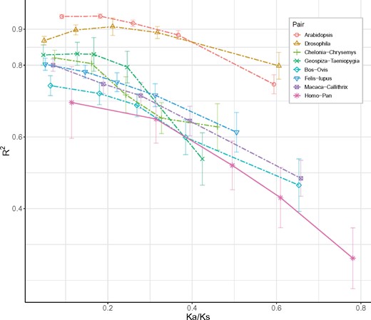
—Relationship between R² values (Obs(Ki/Ks) vs. E(Ki/Ks)) and selection strength (Ka/Ks). Orthologous genes in each pair of species are divided into five categories with equal nonsynonymous changes, according to their Ka/Ks ratio. The x axis is the average Ka/Ks ratio of each category in each species pair and the y axis is the R² value (squared correlation coefficient) of their expected against observed Ki/Ks. The error bars represent the 95% confidence intervals for R².

Open in new tabDownload slide

Discussion

The average pattern of molecular evolution is driven predominantly by negative selection. In most genes of most taxa, Ka/Ks < 0.3, which means the elimination of more than 70% of nonsynonymous mutations. The prevailing negative selection has led to a strikingly simple pattern: Codon evolution takes small steps and follows a nearly universal rule. By this rule, when an exchange between AA1 and AA2 is five times more likely than that between AA3 and AA4 in mammals, the same ratio would be preserved in nonmammalian vertebrates, invertebrates, and plants. The relative magnitude remains nearly constant.

Given the general pattern in such diverse taxa, negative selection at the codon level must be operating at a basic level of biochemistry (Weber and Whelan 2019). We show that the working of negative selection depends on the AA distances, almost all of which contribute to the fitness differences. Even the most obvious properties like hydrophobicity and nonbonded energy contribute only a small fraction to the overall evolutionary rate. Hence, the previous optimism that a small subset of AA distances may explain much of the variation in AA substitutions (Grantham 1974; Miyata et al. 1979) may be untenable.

The simple evolutionary pattern associated with the complex biochemistry provides an important lesson on the physicochemical basis of traits and diseases. There have been many proposals for measuring AA distance as an index of fitness difference (Grantham 1974; Dayhoff et al. 1978; Miyata et al. 1979; Henikoff and Henikoff 1992). Because matrices relying on a few biochemical properties are not likely to capture much of the evolutionary pattern (see fig. 2), it may be more informative to assess the evolutionary rate directly from DNA sequence evolution. In this perspective, the Δ_U measure of codon substitution should be particularly suited to that task (supplementary table S3 and supplementary text V, Supplementary Material online).

In comparison with previous studies that link AA properties with molecular evolution at the codon level (Zuckerkandl and Pauling 1965; Epstein 1967; Clarke 1970; Grantham 1974; Miyata et al. 1979; Kimura 1983; Tang et al. 2004), this study shows clearly the need to separate the effects of negative and positive selection. Indeed, some previous studies have reported unusual AA substitution patterns in extreme environments or under domestication, where positive selection could be prevalent (Lu et al. 2006; Luo et al. 2017; Xu et al. 2017; Chen, Shi, et al. 2019; He et al. 2019; Wang et al. 2017; Wen et al. 2018). Although the working of negative selection is, to some extent, predictable, positive selection may show very different patterns, which is addressed in the accompanying study (Chen, He, et al. 2019).

Supplementary Material

Supplementary data are available at Genome Biology and Evolution online.

Acknowledgments

We would like to thank Ziwen He, Haijun Wen, Hao Yang, Qipian Chen, and members of Wu Lab for discussions and advices. This work was supported by the National Natural Science Foundation of China (31730046 and 91731301) and the 985 Project (33000-18841204).

Literature Cited

Author notes