


Abstract
Following the publication of the Task Force document on heart rate variability (HRV) in 1996, a number of articles have been published to describe new HRV methodologies and their application in different physiological and clinical studies. This document presents a critical review of the new methods. A particular attention has been paid to methodologies that have not been reported in the 1996 standardization document but have been more recently tested in sufficiently sized populations. The following methods were considered: Long-range correlation and fractal analysis; Short-term complexity; Entropy and regularity; and Nonlinear dynamical systems and chaotic behaviour. For each of these methods, technical aspects, clinical achievements, and suggestions for clinical application were reviewed. While the novel approaches have contributed in the technical understanding of the signal character of HRV, their success in developing new clinical tools, such as those for the identification of high-risk patients, has been rather limited. Available results obtained in selected populations of patients by specialized laboratories are nevertheless of interest but new prospective studies are needed. The investigation of new parameters, descriptive of the complex regulation mechanisms of heart rate, has to be encouraged because not all information in the HRV signal is captured by traditional methods. The new technologies thus could provide after proper validation, additional physiological, and clinical meaning. Multidisciplinary dialogue and specialized courses in the combination of clinical cardiology and complex signal processing methods seem warranted for further advances in studies of cardiac oscillations and in the understanding normal and abnormal cardiac control processes.
Introduction
Heart rate variability (HRV) analysis is widely used to characterize the functions of the autonomic nervous system (ANS). Both physiological cardiovascular models and the development of new clinical characteristics benefit from HRV analyses.
In 1996, the Task Force set-up by the European Society of Cardiology and the North American Society of Pacing and Electrophysiology suggested HRV standards. This standardization document1 became widely referenced with more than 5000 citations (Scopus). The 1996 ‘standards of measurement, physiological interpretation, and clinical use’ were related to time- and frequency-domain HRV analysis for short- and long-term recordings (Table 1). Since the publication of the Task Force standards, thousands HRV-related articles appeared. Broadly speaking, they belong to two different categories. Technically oriented articles report new HRV analysis technologies, while medically oriented publications deal with HRV assessment in different physiological and clinical conditions. Unfortunately, there is presently noticeable disconnect between these two categories. Biomedical engineering literature includes many methods that have never been prospectively applied to clinical data. Practical value of advanced novel HRV technologies might thus be difficult to judge.
Standard time- and frequency-domain parameters, as defined by the 1996 Task Force document on heart rate variability. Adapted from Ref. 1
| Variable | Units | Description |
|---|---|---|
| Time domain, statistical measures | ||
| SDNN | ms | Standard deviation of all NN intervals |
| SDANN | ms | Standard deviation of the averages of NN intervals in all 5-min segments of the entire recording |
| RMSSD | ms | The square root of the mean of the sum of the squares of differences between adjacent NN intervals |
| SDNN index | ms | Mean of the standard deviations of all NN intervals for all 5-min segments of the entire recording |
| SDSD | ms | Standard deviation of differences between adjacent NN intervals |
| NN50 count | Number of pairs of adjacent NN intervals differing by more than 50 ms in the entire recording | |
| pNN50 | % | NN50 count divided by the total number of all NN intervals |
| Time domain, geometric measures | ||
| HRV triangular index | Total number of all NN intervals divided by the height of the histogram of all NN intervals measured on a discrete scale with bins of 1/128 s | |
| TINN | ms | Baseline width of the minimum square difference triangular interpolation of the highest peak of the histogram of all NN intervals |
| Differential index | ms | Difference between the widths of the histogram of differences between adjacent NN intervals measured at selected heights |
| Logarithmic index | ms–1 | Coefficient of the exponential curve , which is the best approximation of the histogram of absolute differences between adjacent NN intervals |
| Frequency domain, short-term recordings (5 min) | ||
| Total power | ms2 | Variance of all NN intervals (≈≤0.4 Hz) |
| VLF | ms2 | Power in VLF range () |
| LF | ms2 | Power in LF range () |
| LF norm | LF power in normalized units: LF/(Total power − VLF) × 100 | |
| HF | ms2 | Power in HF range () |
| HF norm | HF power in normalized units: HF/(Total power − VLF) × 100 | |
| LF/HF | Ratio LF/HF | |
| Frequency domain, long-term recordings (24 h) | ||
| Total power | ms2 | Variance of all NN intervals (≈≤0.4 Hz) |
| ULF | ms2 | Power in the ULF range () |
| VLF | ms2 | Power in the VLF range () |
| LF | ms2 | Power in the LF range () |
| HF | ms2 | Power in the HF range () |
| Slope of the linear interpolation of the spectrum in a log–log scale () | ||
For this reason, the e-Cardiology Working Group of the European Society of Cardiology and the European Heart Rhythm Association have jointly charged the authors of this text with researching and summarizing the value of those HRV methods that have not been addressed in the original standards1 while leading to medically relevant results in recent literature. This document has also been co-endorsed by the Asia Pacific Heart Rhythm Society.
Methodology of the study
Increasing numbers of HRV-related publications (Figure 1) are likely facilitated by the ease of collecting RR intervals series and by the availability of different methodologies. This document is based on the position that every new HRV analysis parameter should address some unmet clinical or research need which is not solved by more traditional approaches, and preferably also validated on a solid database of annotated cardiovascular signals. Based on this premise, we identified a number of new methodologies reported in more than 800 publications during the last two decades, and selected those dealing with clinical studies fulfilling all of the following criteria: (i) published in a selected group of clinically relevant high-ranking journals after the 1996 Task Force document; (ii) enrolled at least 200 subjects; and (iii) contained the words ‘heart rate’ and ‘variability’ in the title or abstract. (The journals considered were, in alphabetical order: American Heart Journal, American Journal of Cardiology, American Journal of Physiology: Heart and Circulatory Physiology, Cardiovascular Research, Circulation, Circulation: Arrhythmia and Electrophysiology, Circulation Research, Europace, European Heart Journal, Heart, Heart Rhythm, International Journal of Cardiology, Journal of the American College of Cardiology, Nature, Science, The Lancet, and The New England Journal of Medicine.)

Number of citations returned by PubMed when searching for ‘heart rate variability’ in the title or abstract, for each year between 1980 and 2013. The total of the citations exceeds 10 000.
As of December 2013, some 130 articles fulfilled these criteria. Most of them employed solely the ‘standard methods’ as previously summarized by the Task Force.1 Only 21 studies used ‘non-standard methods’, commonly referred to as ‘nonlinear’. Some of these publications described similar HRV characteristics (Table 2). Heart rate turbulence (HRT), included in 7 of the 21 studies,2–10 was not considered because of the recent independent consensus document.11
Overview of the non-standard metrics in publications fulfilling the selection criteria
| References | Patients | α | DFA α2 | DFA α1 | Poincaré plot | ApEn | DC/AC | HRT | Others |
|---|---|---|---|---|---|---|---|---|---|
| Perkiömäki et al. 20113 Europace | 292 AMI | ✓ | ✓ | ||||||
| CARISMA | <0.77 | ||||||||
| Gang et al. 20114 Europace | 292 AMI | ✓* | ✓ | ✓ | |||||
| CARISMA | >1.5 | <0.9 | |||||||
| Cygankiewicz et al. 200910 Am J Cardiol | 294 CHF | ✓ | |||||||
| MUSIC | |||||||||
| Rashba et al. 200912 Circulation | 300 AMI | ✓ | |||||||
| AET-EP | |||||||||
| Mozaffarian et al. 200813 Circulation | 1152 H ≥ 65 years | ✓ | ✓ | ||||||
| Cygankiewicz et al. 20069 Am J Cardiol | 487 CHF | ✓ | |||||||
| MUSIC | |||||||||
| Beckers et al. 200614 Am J Physiol Heart Circ Physiol | 276 H | ✓ | ✓ | ✓ | ✓ | ✓ (1) | |||
| Bauer et al. 200615 Lancet | 2711 AMI | ✓ | |||||||
| Bauer et al. 20068 Int J Cardiol | 608 AMI | ✓ | |||||||
| EMIAT | |||||||||
| Guzzetti et al. 200516 Eur Heart J | 330 CHF | ✓ | |||||||
| >1.33 | |||||||||
| Hallstrom et al. 20057 Int J Cardiol | 744 AMI | ✓ | |||||||
| CAST | |||||||||
| Wichterle et al. 20042 Circulation | 2027 AMI | ✓ | ✓ (2) | ||||||
| EMIAT + ATRAMI | ≥0.1 | ||||||||
| Osman et al. 20046 Am J Cardiol | 799 BHyT | ✓ | |||||||
| Jokinen et al. 20035 Am J Cardiol | 600 AMI | ✓* | ✓ | ✓ | |||||
| MRFAT | >1.55 | <0.65 | |||||||
| Sosnowski et al. 200317 Int J Cardiol | 594 AMI | ✓ (3) | |||||||
| <35% | |||||||||
| Tapanainen et al. 200218 Am J Cardiol | 697 AMI | ✓ | ✓ | ✓* | |||||
| >1.55 | <1.05 | <0.65 | |||||||
| Mäkikallio et al. 200119 J Am Coll Cardiol | 325 H ≥ 65 ys | ✓ | ✓* | ||||||
| Turku, Finland | >1.5 | <1.0 | |||||||
| Mäkikallio et al. 200120 Am J Cardiol | 499 CHF | ✓ | |||||||
| DIAMOND CHF | <0.9 | ||||||||
| Pikkujämsä et al. 200121 Am J Physiol Heart Circ Physiol | 389 H | ✓ | ✓ | ||||||
| ≈1 | ≈1 | ||||||||
| Huikuri et al. 200022 Circulation | 446 AMI | ✓ | ✓ | ✓* | ✓ | ||||
| DIAMOND MI | >1.5 | <0.85 | <0.75 | SD2<55 | |||||
| Huikuri et al. 199823 Circulation | 325 H ≥ 65 ys | ✓ | |||||||
| Turku, Finland | >1.5 |
Dichotomization thresholds are reported when applicable. An asterisk marks the technique which was comparably better than others. The ‘Patients’ column reports the number and clinical class of patients investigated: H, healthy; AMI, acute myocardial infarction survivors; CHF, congestive heart failure; BHyT, biochemical hyperthyroidism. Where available, the trial name is included. Column ‘Others’ refers to: (1) Fractal dimension, correlation dimension , and largest Lyapunov exponent. (2) Prevalent low-frequency oscillation. The technique, locates the frequency of the predominant peak in the LF band (with similarities to methods which locate the frequency of the predominant pole of an autoregressive model). (3) Heart rate variability fraction, a measure of concentration of the bi-dimensional histogram of consecutive RR intervals (closely related to the Poincaré plot) around a most common pattern.
The following text describes technical aspects of these methods, their clinical achievements, and suggestions for clinical application. Standards of implementation of the methods are proposed in Appendix together with more detailed technical information. This document aims at facilitating the understanding of the advances offered by the new methods in physiological and clinical studies.
Methods description
The following methods satisfied the described criteria: (i) Long-range correlation and fractal analysis; (ii) Short-term complexity; (iii) Entropy and regularity; and (iv) Nonlinear dynamical systems and chaotic behaviour. For each method, we provide the ‘background concepts’ and the ‘contributions to HRV understanding’. All these methods deal with the time series of normal-to-normal RR interval (NN intervals).
Long-range correlation and fractal scaling
Many methods have been proposed to estimate the fractal-like behaviour of HRV.24 The most representative methods are the power-law exponent of the spectrum and the detrended fluctuation analysis (DFA) long-term exponent .
Background concepts
The term fractal is most often associated with geometrical objects. It describes an entity too irregular for traditional geometrical shapes (fractional dimensionality) which shows some degree of self-similarity. That is, it resembles a common pattern when seen on different scales. Analogously, a temporal stochastic process is said to be self-similar, when its fluctuations on small time scales are statistically equivalent to those on large time scales. Mathematically, this is formalized by requiring that time series and have identical statistical properties for a certain range of scales . The real number is called the scaling exponent and characterizes the self-similarity of series .
Fractal properties of NN series have been extensively researched.24,18,25–29 Fluctuations on multiple scales make fractal time series seemingly irregular. In fractal analysis, NN series are considered generated by a random stochastic process (such as tossing of a coin) rather than by a deterministic system (such as implementing a precise mathematical equation).
Self-similar signals display a power-law spectral density30 in the very low-frequency range. The exponent of the pattern measures the self-similarity scaling (Figure 2). The generalized correlation function of fractal NN signals decays very slowly, implying that the contemporary value of the series is significantly affected by its past. The self-similar (fractal) processes are also often referred to as ‘long-memory’ or ‘long-range dependence’ processes. Non-stationary self-similar processes display a variance increasing with the length of the series. The so-called DFA allows quantifying the process by measuring how the variance is affected by the length of the NN series.
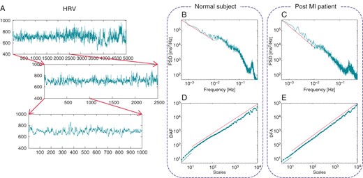
Self-similar tachograms resemble a common pattern when inspected on different scales (A). Self-similarity manifests itself into a power-law power spectral density (PSD) in the very low frequency (B and C) and DFA for long scales (D and E). The scaling does not continue indefinitely as frequency increases (or scale decreases) and breaks down when the other typical HRV spectral components become dominant (e.g. the peak in the PSD at about 0.3 Hz). Self-similarity is affected by many pathological conditions like myocardial infarction. The healthy subject in (B) and (D) has α = 1.07 and DFA long-term exponent = 1.04 while the post-MI patient in (C) and (E) has α = 1.44 and . The linear scaling of the short-term DFA exponent is also included in (D) and (E) for scales ≤11 ( and 1.08, respectively).
More recent studies dealt with a higher order approach, called multifractal analysis in which a fractal is composed by a set of fractals.31,32 Different sub-parts of the signal are characterized by local regularities with different fractal dimensions. While the theoretical framework is rather complex, multifractal signals are in practice characterized by more than one scaling coefficient .
Contribution to heart rate variability understanding
Self-similar (fractal) measures provide quantitative description of irregularities present in physiologic signals. Contrary to spectral techniques, fractal analysis studies the irregularity of the NN series assuming that it is not characterized by any fixed time scale.
Similar to other system studies, the main limitation of fractal analysis is the lack of direct correspondence to physiology. Changes of scaling exponent observed in different clinical conditions are not specific for underlying physiologic and/or pathologic mechanisms.
Short-term complexity
Background concepts
While fractal analysis quantifies long-term irregularity, these techniques quantify irregularities on shorter scales (at most 10 NN intervals). The short-term analysis reflects both the continuous adaptations of several regulatory processes operating at different time scales, and the different capacity for cardiovascular adaptation over different short scales.25,33 There are several methods in this category differing in their value for HRV analysis.
Contribution to heart rate variability understanding
Detrended fluctuation analysis short-term exponent
Detrended fluctuation analysis is derived from fractal analysis and is suitable for processing of scale-invariant signals (i.e. signals showing the same statistical properties on a broad time-scale range). Already seminal applications showed that HRV has different properties on short or long scales.
The DFA short-term exponent estimates the self-similarity properties of HRV on short scales (Figure 2) and is highly effective in clinical applications (Table 2). However, it does not describe the overall self-similarity characteristics of HRV. Nevertheless, it seems suitable to quantify short-term changes caused by NN interval oscillations that may be affected by autonomic activation34,35 and are often wrongly related solely to respiration.
Poincaré plot analysis
A Poincaré plot (or recurrence map) is obtained by simplistically plotting the values against the values of . The name stems from dynamical systems theory (a Poincaré map is a reduction of a N-dimensional continuous system to a (N – 1)-dimensional map,36 see also ‘Nonlinear dynamical systems and chaotic behaviour’ section).
In HRV applications, the mainstream usage of Poincaré plots has been limited to a ‘tool for graphically representing summary statistics’37 with little connections to nonlinear dynamical systems theory (Figure 3). Typical parameters derived from Poincaré plots, such as SD1, SD2, or SD12 (see ‘Poincaré plot analysis’ section in Appendix) are directly related to standard temporal indices SDNN and SDSD37 and provide the same information. The sole benefit of visual analysis of Poincaré plot is in confirming the adequate editing of the NN interval series, e.g. separating ectopic beats from random oscillations of sinus beats without compensatory pauses (Figure 3B).
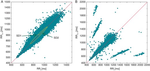
Traditional parameters obtained from a Poincaré plot (A). SD1 and SD1 are mathematically equivalent to linear HRV indices (‘Poincaré plot analysis’ section in Appendix). Poincaré plots are effective in detecting errors in the labelling procedure, ectopic beats, or other rhythm abnormalities as shown in (B).
Heart rate variability fraction17 has been proposed as a measure of concentration of the bi-dimensional histogram of RR intervals (a discretized Poincaré plot).
Deceleration and acceleration capacity
The underlying hypothesis of these analyses is that heart rate changes due to a particular trigger event are repetitive. Phase rectified signal averaging (PRSA) selects instances of particular events, aligns them in phase, and performs signal averaging of the time series to extract the information of interest.33,38 Phase rectified signal averaging thus allows detecting and quantifying oscillations masked by the non-stationary nature of the analysed signal. The simplest events in the NN series are when heart rate decelerates or accelerates.15 By using these two triggers, the PRSA allows to quantify deceleration-related (deceleration capacity—DC) and acceleration-related (acceleration capacity—AC) modulations of NN series separately. The same averaging method may be used to study interactions of different signals (e.g. blood pressure, respiration) with NN series.39
Entropy and regularity
Background concepts
In physics, entropy describes, loosely speaking, the amount of ‘disorder’ of particles in a system. In information theory,40entropy relates to the probability density function of a variable. When applied to a sequence (e.g. using a histogram), it is often termed ‘Shannon’ entropy and quantifies its complexity by means of an average information content. The entropy rate measures the increase of entropy of a sequence when an extra sample is added. Clearly, if the entropy rate drops when the sequence grows, the process is very regular and predictable. Conversely, a constant entropy rate suggests that each new sample is not completely predictable (Figure 4). In HRV analysis, the entropy rate is often simplistically referred to as ‘entropy’.
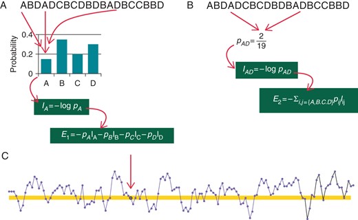
Schema of entropy in the HRV context. The quantity of information carried by an event is computed as the logarithm of its inverse probability: rare events (low probability) carry large informative contents. (A) A tachogram in which NN intervals was classified into four possible classes, labelled A–D. To compute the information carried by class A, the probability of the class is first estimated by an histogram. Then the (Shannon) entropy of the NN series is obtained as the average of the information provided by each NN class. The same can be done for any number of consecutive NN interval classes (B for ). Entropy rate measures how much entropy changes from to , i.e. . Approximate entropy and SampEn estimate the entropy rate of the NN series (C). Instead of building an histogram of NN durations, the number of intervals which do not differ more than from a given NN interval (arrow) are counted (highlighted area in C).
Metrics such as approximate entropy (ApEn) and sample entropy (SampEn) were proposed to quantify the entropy rate of short- to mid-length NN series. The conditional corrected entropy (CCE) provides similar information after NN intervals of similar length are represented with a common label (the so-called ‘symbolic representation’, ‘Symbolic dynamics’ section in Appendix).
Contribution to heart rate variability understanding
The ANS adapts the heart rate to the current needs which might change continuously. Thus, the NN series is irregular with high entropy. However, when the system becomes less responsive to environmental stimuli, entropy decreases and the NN signal becomes more ‘ordered’. Highly ordered (low entropy) signals are more predictable than low ordered (high entropy) signals. Entropy measurements are particularly sensitive to transient irregularity and changes in HRV, especially in short-term recordings.39,19
Approximate entropy, SampEn, and CCE were shown to progressively decrease during sympathetic activation induced by gradual head-up tilt test,41 thus offering an alternative measurement of sympathovagal balance.
Nonlinear dynamical systems and chaotic behaviour
Over short time scales, autoregressive models of NN series are generally suitable for statistical prediction and studies of the underlying evolution of physiological systems42 if no abrupt changes alter the physiologic regulation. In long series, however, abrupt changes may occur frequently. Then, a ‘dynamical’ system analysis might be used, where the position-in-time (or ‘trajectory’) of a point within a geometrical (or ‘state’) space, is determined by a fixed mathematical law specifying the immediate future. The coordinates of the point are called ‘state variables’ and their number defines the dimension of the system (the ‘degrees of freedom’). Unless the dynamical rule is a linear combination of state variables, the system is called a nonlinear dynamical system. Many biophysical phenomena can be modelled as dynamical systems.
Theories of nonlinear dynamical systems and of chaotic behaviour may be used to study the HRV predictability and complexity. In such studies, NN series represents the output of a ‘nonlinear’ dynamical system (Figure 5).
![(A) Approximately 4 min. of NN series of a healthy subject embedded in a space of M dimension (M = 3). Each point is constructed by taking delayed samples of the HRV series, XM(i)=[NNi,NNi+1,NNi+2]. Under the hypothesis that HRV is dictated by a low-order nonlinear system, the reconstructed trajectory is used to infer properties of the unknown system. In a chaotic nonlinear system, distance between nearby trajectories grows exponentially with time (B). The growth rate is modulated by the largest Lyapunov exponent λ1 and this property is often expressed as ‘large sensitivity to initial conditions’. Even if trajectories are forced to diverge they are also bounded to a subspace: the attractor. To stay bounded they need to ‘fold back’. Since they cannot cross each-other, they often wander over a fractal geometrical entity.](https://oup.silverchair-cdn.com/oup/backfile/Content_public/Journal/europace/17/9/10.1093/europace/euv015/2/m_euv01505.jpeg?Expires=1750276451&Signature=z6ViyjoHBFagVG6z9g1NV6XmqSgVWAaB0MjfP-yJ41ad65CQpKTNdYZPxSW-jlqp488Sna0LSR7mb5BWoMSYvROqGLLzS0Yvwscm1U150X7n9c542OvXLEfWQktbcChaJZ12GpbgHCx5e8z-qoseDl0kbxU5S-zL5-ZM7dmRB0w28nohjpgxTFrW0tE1NAhkcvHnjqW15JuacvyIcc7xzZraCPKi4UXE3oH-oBnu~DtfGPnfhOE2barpL3cl3GOUPwC6gDGaQQQXNg8U0M1jG2VgMwBdV60Sx1YLrAcWRREN-t6kceFXLMS6e-utLYacetrtYcZVUi7ukLeO01iifg__&Key-Pair-Id=APKAIE5G5CRDK6RD3PGA)
(A) Approximately 4 min. of NN series of a healthy subject embedded in a space of M dimension (M = 3). Each point is constructed by taking delayed samples of the HRV series, . Under the hypothesis that HRV is dictated by a low-order nonlinear system, the reconstructed trajectory is used to infer properties of the unknown system. In a chaotic nonlinear system, distance between nearby trajectories grows exponentially with time (B). The growth rate is modulated by the largest Lyapunov exponent and this property is often expressed as ‘large sensitivity to initial conditions’. Even if trajectories are forced to diverge they are also bounded to a subspace: the attractor. To stay bounded they need to ‘fold back’. Since they cannot cross each-other, they often wander over a fractal geometrical entity.
Background concepts
Nonlinear dynamical systems might show sensitive dependence on initial conditions (Figure 5). That is, limited error in the knowledge of the initial state leads to an ‘unlimited’ error in the orbits. Such systems are called chaotic.36 They are characterized by a positive Lyapunov exponent, which is a mathematical measure of the rate of divergence of neighbouring trajectories. Another usual characteristic of nonlinear dynamical systems is that trajectories at equilibrium are often limited by a ‘strange’ attractor (a geometrically fractal entity).
Since the initial proposal of chaotic nature of human HRV,43 many attempts have been made to find the evidence of chaos. After reconstructing the trajectories of the hypothetical system, investigations looked for (i) a positive Lyapunov exponent, (ii) a non-integer correlation dimension D244 or fractal box-counting dimension of the attractor, and (iii) a decrease in nonlinear predictability, and other characteristics.
Contribution to heart rate variability understanding
The results collected so far are very limited. Glass recently clearly summarized:45 ‘Although there have been some spectacular advances in understanding the nonlinear dynamics of complex arrhythmias, the application of these insights into clinically useful procedures and devices has been more difficult than I imagined’.
Possible explanations for these inconclusive findings include the sensitivity of investigated measures (i.e. Lyapunov exponent and ) to the limited length and noise of NN series.46 Also, long-range correlated random processes (stochastic, hence non-chaotic) which also possess fractal properties (‘Long-range correlation and fractal scaling’ section), easily produce false positive test-results for deterministic chaos. Thus, in our opinion, it is impossible to draw the conclusion that human HRV arises from a chaotic behaviour of the cardiovascular system.45 However, techniques (or their variants) developed in the context of nonlinear dynamical system were successfully employed to characterize HRV irregularity and in risk stratification.47,48
Clinical achievements
The novel approaches characterizing complex systems require sophisticated theoretical and computational background. This restricts successful application of the new methods to centres with advanced knowledge in both medical and engineering/computer science fields. So far, this prevented widespread clinical utilization of these methods.
Although it is possible to hypothesize theoretically that some of the new metrics quantify HRV characteristics, such as self-similarity and complexity, which cannot be explored by traditional methods, clinical advances of the new methods are not entirely supported by the presently available data.
Myocardial infarction
Bigger et al.49 were the first to report the clinical relevance of (‘Long-range correlation and fractal scaling’ section) after acute myocardial infarction (AMI). In a survival analysis, was linked to increased mortality during follow-up.
Subsequently, Huikuri et al.22 reported that in AMI survivors with left ventricular ejection fraction (LVEF) , (and also DFA ) was superseded by DFA as the most powerful predictor of all-cause mortality, after adjusting for other factors including age, LVEF, NYHA class, and medications.
These findings were confirmed by Tapanainen et al.18 who also showed that DFA was the most powerful predictor of mortality among AMI survivors. In a subsequent study by the same group,5 multivariate analysis showed that, after adjustment of clinical variables, DFA and (as well as HRT slope and onset) predicted subsequent cardiac death. The predictive value of both parameters was retained when measured at the convalescent or late phase after AMI.
No significant differences at 1 year were also found in DFA changes between patients randomized after AMI to receive percutaneous coronary intervention and stenting or optimal medical therapy alone.12
CARISMA substudy4 noticed that power-law exponent was the most effective HRV-related risk predictor of developing high-degree atrioventricular block after AMI. Subsequently, in another CARISMA substudy,3 DFA adjusted for relevant clinical variables, was a significant predictor of ventricular tachyarrhythmias.
Available evidence thus suggests that DFA short-term exponent might be an effective predictor of cardiac death whilst self-similarity properties of the NN series over long period of time (e.g. power-law exponent ) might be a more general predictor of all-cause mortality. This is consistent with the fact that the properties of long-term recordings reflect a combination of different control mechanisms and are thus affected by both cardiac and extra-cardiac factors. On the contrary, analysis of short-term recording reveals the failure to adapt to cardiac stimuli, such as transient myocardial ischaemia, with implications for cardiac prognosis.
In respect of the predictive values of Poincaré plots, was a significant predictor of all-cause and non-arrhythmic cardiac mortality in AMI survivors,22 after adjustment for traditional risk factors (age, LVEF, NYHA class, and medication). The same study showed that traditional HRV parameters, including VLF and LF power, displayed similar or higher predictive values. The additional clinical value of Poincaré plot analysis is thus limited.
Deceleration capacity was evaluated in a large multicentre study15 of post-AMI patients and proved to be a better predictor of mortality than LVEF and SDNN. In addition, when dichotomized at 2.5 ms, DC was the highest relative predictive risk parameter in a multivariate Cox regression analysis. Deceleration capacity was also shown of increased clinical value when combined with HRT.50
Finally, Voss et al.51 reported that the high-risk prediction after AMI by traditional time- and frequency-domain HRV parameters was further improved by the addition of symbolic dynamics.
Congestive heart failure
In the DIAMOND study patients, Mäkikallio et al.20 reported that DFA , together with conventional HRV parameters, predicted mortality univariately. After age, functional class, medication, and LVEF adjustment, DFA remained an independent mortality predictor, also in patients with most severe functional impairment.
In a large congestive heart failure (CHF) population, Guzzetti et al.16 reported that the power-law exponent was significantly univariately related to the extent of ventricular dysfunction in whereas traditional spectral parameters (VLF components in particular) had greater prognostic value. In multivariable analyses, was no longer a significant risk predictor.
In a study comparing the predictive value of several HRV nonlinear parameters in CHF patients, Maestri et al.48 showed that only symbolic dynamics added prognostic information to traditional clinical parameters. More recently, DFA has been confirmed affective in predicting cardiovascular death in GISSI-HF population,52 also when taking into account traditional clinical variables and HRV parameters.
Thus, in CHF, where HRV is known to decrease and to reflect disease progression, novel short-term measures provide quantitative description of the residual variability but their advantages in clinical studies of risk prediction are at best modest.
Subjects without evidence of heart disease
Huikuri et al.23 reported that a value of was the best predictor of all-cause mortality in a large population of subjects over 65 years of age, even after adjustment for several clinical parameters. Subsequently, Mäkikallio et al.19 showed that DFA was an independent predictor of sudden cardiac death among HRV-related indexes whereas the power-law exponent was the strongest predictor of all-cause mortality. Mozaffarian et al.13 confirmed the association of DFA with cardiac death risk (after adjusting for age, gender, race, education, smoking, diabetes, treated hypertension, and body mass index) and also showed, that fish consumption ( fatty acids) was significantly correlated with DFA Finally, in a large community-dwelling adult population (age 65–93 years), the combination of low DFA with abnormal HRT was a strong risk factor for cardiovascular death even after adjustment for conventional cardiovascular risk parameters.53
Beckers et al.14 studied age effects in a population of healthy subjects with ages between 18 and 71. Both and DFA increased with age, whereas gender differences were less pronounced.
In subjects with no evidence of heart disease and history of paroxysmal atrial fibrillation, ApEn was found to decrease before the onset of arrhythmic events.54 Sample entropy also predicted sepsis in prematurely born infants.55
Suggestions for clinical use
The following suggestions aim at placing the utility of the novel HRV technologies in the appropriate context.
Notwithstanding the new methods described in this text, traditional time and frequency-domain HRV analysis remain the methods of choice for the assessment of ANS physiology and pathophysiological modelling. In fact, the long experience and validation of traditional techniques make them the most reliable tools. Therefore, we suggest using the new techniques in conjunction with more traditional ones, to enrich our physiological and clinical understanding of the mechanisms underlying HRV. Available data indicate that these novel methods have provided more information on the complexity and mathematical or physical characteristics of the variability signal than on sympathetic or parasympathetic neural control mechanism, even if they were originally developed to clarify the physiological correlates of HRV.
As with traditional HRV techniques, the recording conditions (duration, body position, free or controlled breathing, etc.) can substantially affect short-term metrics, thus making comparison of different studies challenging. There is also limited information on the reproducibility of new methods. Studies performed on small subjects population hint that the intra-subject repeatability for short-term metrics is comparable with that of traditional HRV indexes, but further evidence is necessary.
Available studies of post-AMI risk suggest that short-term fractal scaling (DFA ) may successfully predict cardiac mortality while other novel methods appear to predict all-cause mortality. Nevertheless, available comparisons of the traditional and novel HRV analyses do not show consistent superiority of the new methods in clinical risk stratification studies. Systematic statistical evaluation of the additive prognostic value of the new methods is presently lacking. Comprehensive comparisons of the traditional and novel methods are needed based on new prospective clinical studies and/or meta-analyses of large existing databases. Without such comparisons, widespread use of the novel methods in clinical risk studies cannot be recommended.
Although in CHF patients, short-term DFA measures appear effective in identifying high-risk patients, there are many categories of clinically well-defined populations in which the use of novel HRV techniques has not been attempted.
Similar to the conventional HRV methods, the results of the new methods are affected by age. The extent and the character of this age dependency are less known compared with that of the conventional HRV methods. In physiologic and clinical studies, age dependency should therefore be carefully considered, e.g. by including age-matched control groups.
Conclusions
The novel approaches to HRV analysis summarized in this text contributed in the technical understanding of the signal character of NN sequences. On the other hand, their success in developing new clinical tools, such as those for the identification of high-risk patients, has been so far rather limited. Some of the novel parameters correlate with more traditional measurements, demonstrating a consistency that, nevertheless, does not allow substituting the latter with the former. In many instances, however, the new parameters seem to provide different information about the complexity of the physiological underlying mechanisms which constitutes an important step for the future. The physiological and clinical impact of the observed physical signal processing properties seems to still suffer from the conceptual disconnect between clinical cardiologists on the one side and mathematicians and engineers involved in signal processing theories on the other side. At the same time, available results obtained in selected populations of patients researched by specialized laboratories are of interest and potential promise. Multidisciplinary dialogue and specialized courses in the combination of clinical cardiology and complex signal processing methods seem warranted for further advances in cardiac physiology and in the understanding normal and abnormal cardiac control processes. Additional clinical validation of existing novel methods is needed in multicentre studies with large cohorts of patients to define their clinical predictive value as well as their robustness in relation to reproducibility, clinical widespread use, and possibly, implementation in commercial devices. Before such validations are available and before the clinical use of existing novel techniques becomes more widespread, it is difficult to encourage the development of new variants of the novel methods or of completely new methods based on highly sophisticated signal processing techniques. Signal processing HRV techniques that do not reflect unmet clinical needs are of little value irrespective of the depth of their mathematical apparatus.
Appendix
Implementation standards
Long-range correlation and fractal scaling
1/f power-law exponent α
Two main computational strategies for the power-law exponent α were proposed. The earlier one22,19,23 was used by Bigger et al.49,56 It requires resampling the NN series to obtain a regularly spaced time series. Subsequently, the power spectrum (FFT-based) is integrated (‘logarithmic smoothing’) over frequency with an equal number of bins per decade (60 bins/decade). A robust regression is applied in the log(power) vs. log(frequency) axis, in the range of 10–4 < f < 10–2 Hz. The slope of this line is the scaling exponent . The other method is described in the 1996 Task Force document1 and is analogous to the first one except that the NN series is not resampled and the logarithmic smoothing is not performed. Both methods are technically equivalent. The logarithmic smoothing (sometimes called ‘boxed’ or ‘modified’ periodogram method) was introduced to compensate the unevenly distribution of points in the log(frequency) axis and the possible bias due to the larger number of points at the higher frequencies.30,57 However, technical studies validating the long-term scaling exponent estimators on synthetic series of known properties have shown that compared with the simple periodogram method, estimates obtained with logarithmic smoothing lead to slightly larger variance57 or bias.58,59 The fitting range 10–4 < f < 10–2 is a de facto standard, and is in principle preferable to .1
Detrended fluctuation analysis long-term exponent
The DFA algorithm was described in Peng et al.,25 with small additions in Peng et al.,60 and a practical implementation becomes soon available.61 As a result, the computation has been fairly consistent in the literature. Only one detail needs discussing. The range of scales employed to compute DFA in Huikuri et al.22 and Beckers et al.14 is smaller than that proposed in the introduction of DFA.25,26 The upper scale limit is implicitly imposed by the DFA software to one-fourth the length of the input series, and it is seldom reported.24,26 Detrended fluctuation analysis was introduced to reduce the bias possibly produced by spurious non-stationarity when estimating the scaling exponent in stationary self-similar time series. However, in comparative analysis, it performed similarly to the simple periodogram method described in the previous section.57,59
Remarks
The two metrics and DFA are meant to quantify long-range dependence in a given series. However, they operate differently. Detrended fluctuation analysis is directly related to the self-similarity scaling exponent which it estimates (, for , while for ). A scaling relation must be used to obtain a corresponding estimate of the slope of the spectrum for frequencies close to zero, .24,59 Similarly, an equivalent scaling exponent can be obtained from α ( for , while for ).
The fractal dimension is related to by the algebraic relation .
Both the periodogram method and DFA provide estimates linearly related to in the range of physiological interest (typically between 1 and 2). It may thus serve as the reference benchmark techniques.
Finally, fractal analysis is preferable for NN time series from long-term recording (e.g. 24 h and longer).
Short-term complexity
Detrended fluctuation analysis short-term exponent
The short-term DFA scaling exponent is obtained using the same computational steps employed for the long-term DFA exponent . However, the range of scales is different, typically between 4 and ∼11.14,21 The lower bound is the smaller scale allowed by the standard code.61 Although short time scales might contain broad-band noise induced by electrocardiogram (ECG) sampling,31 the results reported in Table 2 suggest that it is not too important.
Poincaré plot analysis
Quantitative analysis of Poincaré plot is typically performed62 fitting an ellipse to the plot. In practice, a new axis is aligned with the line-of-identity. The standard deviation of the cloud of points in the direction traverse to the line-of-identity is usually called SD1, and it is a measure of short-term (‘instantaneous’) HRV. On the contrary, the standard deviation of the cloud of points in the direction of the line-of-identity is termed SD2 and it is a measure of long-term (‘continuous’) HRV. The ratio SD1/SD2 is then termed SD12.
The SD12 ratio was empirically found to be highly correlated with DFA in a large study of subjects aged 65 years and above.13
Deceleration and acceleration capacity
Deceleration capacity and AC computation depends on three parameters: T acts on the selection of the anchor points (the trigger events located on the ECG), L is the width of the averaging window, and s is the number of acceleration/deceleration cardiac cycles. Usually but not always s = T (e.g. T = 1 and s = 2 in Bauer et al.15). In first approximation (the superposition principle does not hold with a nonlinear metric), the values of s and T implicitly enhance HRV oscillations of certain frequency bands, the larger their values the smaller frequencies emphasized. It is sufficient that L > max(T, s).
Remarks
Short-term measures of complexity, such as the DFA short-term scaling exponent and ApEn, were found to show relatively little inter-individual variation in sufficiently large populations and proved more normally distributed that SDNN and spectral measures.27 They also showed an intra-subject repeatability, comparable with that of the mean NN interval65 although their absolute values decrease with advancing age.14 Gender-related differences were reported for these indices14 but without substantial relation to gender-related differences in cardiovascular risk factors in healthy subjects.27
Entropy and regularity
Approximate and sample entropies
Approximate entropy66,67 was originally devised as a practical implementation of the Kolmogorov–Sinai entropy of a nonlinear dynamical system. It can also be seen as an approximation of the differential entropy rate68 of a process. More recently, SampEn69 was introduced to improve over ApEn. Sample entropy converges more rapidly (when computed on shorter series) at the expenses of a larger variance of the estimates.
Approximate entropy and SampEn measure the likelihood that runs of templates that are close for points remain close (less than a certain tolerance level ) for points in a given sequence of length . Small values of ApEn or SampEn identify more regular, predictable, processes. There is no fail-proof rule for the selection of the parameters r and m. Values of r between 10 and 25% (usually 20%) of the standard deviation of HRV are typically employed. For template length, is often used; is used with very short time series.
Symbolic dynamics
Symbolic dynamics try to recognize a general tendency of the NN series by reducing its complexity.70–72 The idea is to associate symbols to states of the ANS, and then quantify the complexity of their evolution in time (i.e. their entropy). In practice, the range of possible NN values is subdivided into a certain number of levels and each NN sample is mapped with a symbol representing the corresponding level. consecutive symbols are grouped together to create a word. The complexity of the signal is assessed computing either the Shannon entropy of the sequence of words or the CCE (an entropy rate).71 There is no definite rule for the selection of the number of levels or length of words . Typically, or and are used (which corresponds in first approximation to computing ApEn with and ). Combination of words is also possible.71
Nonlinear dynamical systems and chaotic behaviour
The analysis starts with the reconstruction of the system trajectories in a phase space from a single HRV record. The common strategy is to construct an M-dimensional trajectory vector by taking delayed samples of the HRV time series , such that , where is a selected fixed lag.73
The largest Lyapunov exponent, the average exponential growth rate of the initial distance between two neighbouring points in as time evolves, is often practically estimated.74 A positive Lyapunov exponent is the hallmark of a chaotic system. First, it quantifies the rate at which a system creates information by increasing the degree of uncertainty about the initial conditions with increasing time steps, or the so-called Kolmogorov–Sinai entropy, of which various real-world estimates have been used to characterize HRV complexity. Secondly, it relates to fractal geometry of phase space trajectories and to non-integer dimensional estimates, such as correlation dimension . Finally, it also relates directly to abrupt drops in nonlinear predictability, due to the exponential growth of the variance of the error between observed and predicted values. Short-term prediction is possible in chaotic systems due to their deterministic nature. The term complexity, different from ‘irregularity’ of stochastic systems, is often used to describe a dynamic change in the predictability. A widespread measure of fractal dimension of the manifold enclosing the trajectories of nonlinear dynamical system is the correlation dimension.44,75
