


Abstract
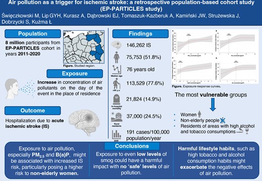
Short-term effects of Polish smog, particularly benzo(alpha)pyrene [B(a)P], are unclear. We aimed to examine the association between short-term exposure to air pollution and ischaemic stroke (IS) incidence.
We conducted a retrospective population-based cohort study including an EP-PARTICLES cohort of 8 million inhabitants in the years 2011–20 (80 million person-years of observation). Individual clinical data on emergency hospitalizations due to IS (ICD-10: I63.X) was analysed. We used quasi-Poisson models to examine municipality-specific associations between air pollutants and IS, considering various covariates. We recorded 146 262 cases of IS with a dominance of females (51.8%) and people over 65 years old (77.6%). In the overall population, exposure to PM2.5, NO2, B(a)P, and SO2 increased the risk of IS onset on the day of exposure by 2.4, 1, 0.8, and 0.6%, respectively. Age and sex were modifying variables for PM2.5, NO2, and B(a)P exposure with more pronounced effects in non-elderly individuals and women (all Pinteraction < 0.001). Residents of regions with high tobacco and alcohol consumption were more sensitive to the effects of PM2.5 and SO2. The slopes of response–effect curves were non-linear and steeper at lower concentrations.
Exposure to air pollution may be associated with higher IS incidence, particularly posing a higher risk to non-elderly women. Harmful lifestyle habits might exacerbate its impact. Exposure to even low levels of air pollutants had negative effects.
The study was registered at ClinicalTrials.gov (NCT05198492).
Lay Summary
The present study aimed to analyse the association between exposure to air pollution and IS incidence:
Exposure to even low levels of air pollution, including B(a)P, might be associated with higher IS incidence, and characteristics of the patients or their place of residence can modify its effect.
The most vulnerable phenotype is non-elderly woman, and harmful lifestyle habits, such as smoking and drinking alcohol, can further increase the negative effects of air pollution.
Introduction
Ischaemic stroke (IS) remains an ongoing threat to public health, being responsible for over 6 million deaths annually worldwide, making it the second most common cause.1 Among people younger than 70 years old, its age-specific prevalence and incidence between 1990 and 2019 rose by 22 and 15%, respectively.1,2 Moreover, according to the Global Burden of Disease study, the largest increase in risk exposure between 2010 and 2019 was for air pollution.3 Ambient particulate matter (PM) was recognized as the fourth leading risk factor for stroke worldwide, annually accountable for nearly 29 million disability-adjusted life years (DALYs).1 Nevertheless, the AHA/ASA 2021 Guideline for the Prevention of Stroke does not mention the impact nor methods of coping with exposure to air pollution concerning IS.4 In contrast, the 2021 ESC Guidelines on cardiovascular disease prevention in clinical practice focus attention on environmental issues, but state that the level of evidence remains weak.5
Recently, evidence for a new type of air pollution was established in the scientific literature—Polish smog.6–11 This primarily occurs in Eastern Europe, characterized by high levels of PM and benzo(alpha)pyrene [B(a)P], with its formation facilitated by low temperatures and high atmospheric pressure, and in prior scientific reports was characterized by particularly negative cardiovascular effects.6–8,10,11 The eastern part of Poland, being one of the poorest regions in Europe, is characterized by suboptimal heating choices in households during the cold season. This suggests that the characteristics of the region itself, as well as its inhabitants, have a significant impact on air quality, and the potential determinants of Polish smog, with appropriate interventions, can be mitigated. The long-term impact of air pollution on cardiovascular diseases (CVDs) has been well established in the scientific literature; however, short-term effects have not been yet well studied, especially in relation to Polish smog and IS incidence in the region of Eastern European. In one meta-analysis, Shah et al.,12 out of the 28 analysed countries, none were located in Central and Eastern Europe. Understanding these dependencies is exceptionally important for healthcare planning and resource allocations. Furthermore, studies conducted in various regions of the world, examining the relationship between exposure to different types of air pollution and CVD, addressing the most vulnerable populations, can contribute to the further development of guidelines for the prevention of CVD in terms of environmental risk factors.
The primary objective of the present study was to assess the association between short-term exposure to air pollution and IS incidence. The secondary objectives were to analyse exposure–response curves, the annual trends of air pollution effects, and the sensitivity of various social groups to the exposure to air pollution depending on individual patient characteristics and their place of residence.
Methods
Study design
We performed a retrospective population-based cohort design. The study design is detailed below and presented in Figure 1. This study was conducted following the STROBE protocols for observational studies, with the STROBE checklist available as Supplementary material online, Table S1. The study design incorporated a dual-validation process where the data sets were independently verified by at least two researchers. This approach ensured the robustness and reliability of the data, providing confidence in the study’s findings. We defined the primary outcome as the incidence of IS. The primary exposures were air pollutants [PM2.5, NO2, SO2, O3, B(a)P, and CO]. The primary model adjustments were selected based on clinical relevance and statistical criteria, including meteorological factors (temperature, relative humidity, and atmospheric pressure), day of the week, public holidays, and infection seasons, to control for potential confounders and ensure the robustness of the findings. Our analysis was conducted on individual-level data. Timeline of the study is presented in Supplementary material online, Figure S4.
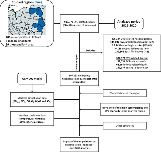
Study design. ACS, acute coronary syndromes; CVD, cardiovascular disease; GEM-AQ, Global Environmental Multiscale Air Quality; km, kilometre.
Studied region
The studied region of Eastern Poland consists of 5 voivodeships, 101 counties, and 709 municipalities. It is inhabited by over 8 million people and its area exceeds 99 000 km2. It is characterized by low industrialization and high agricultural development. Contrasted with the western part of Europe, it exhibits not only a lower socioeconomic status of residents but also a greater number of smaller towns and villages. The map of the studied region is demonstrated in Figure 1 and Supplementary material online, Figures S1 and S2, whereas characteristics of the studied region are available in Supplementary material online, Tables S2–S4.
Hospital admission data
Individual clinical data on hospitalization were obtained from the provincial branches of the National Health Fund in Poland. The study encompassed all emergency (admission codes 2 and 3) admissions on individual level to the hospital diagnosed with IS (ICD-10 code: I63.X) in the years 2011–20 in the analysed region. Ischaemic stroke was defined as the presence of typical neurological symptoms lasting longer than 24 h and the evidence of infarction. Diagnoses were made by attending physicians in respective hospitals based on clinical symptoms and imaging. Patients were hospitalized in hospitals of each reference level and included in the study regardless of the treatment method. The data exhibited high quality, including information on individual level: sex at birth, age, place of residence, in-hospital mortality, and type and date of admission/discharge. The IS-related standardized hospitalization rate (SHR) for all individual counties is available in Supplementary material online, Figure S2.
Air pollution data
In partnership with the Institute of Environmental Protection-National Research Institute, we employed the Global Environmental Multiscale Air Quality (GEM-AQ) model for additional estimations.13 Average daily levels of air pollutants were calculated using municipality resolution grids. This semi-Lagrangian chemical weather model combines air quality mechanisms with tropospheric chemistry within weather forecasting.13 Hourly outputs from the surface layer were aggregated to derive the annual average. To mitigate the low resolution of the air quality monitoring stations, we used the GEM-AQ model, which allowed us to obtain environmental data for all 709 analysed municipalities in high resolution for every analysed day. The concentrations of all analysed air pollutants in individual counties of the analysed region are presented in Supplementary material online, Figure S1.
Weather condition data
Meteorological data were sourced from the Institute of Meteorology and Water Management in Poland. Measurements were systematically carried out within a standardized meteorological enclosure and recorded automatically at predefined intervals. Stringent protocols were implemented to ensure high precision in data accuracy, with temperature and pressure readings maintained at a resolution of 0.1 (degree Celsius or hectopascal), and humidity measurements achieving a precision level of 1%. Weather condition data are available in Supplementary material online, Table S6.
Statistical analysis
The assessment of variable distribution was conducted through the Shapiro–Wilk test. We did not apply any data management strategies due to the absence of missing data. For continuous non-normally distributed variables, the presentation was in the form of median (Me) values with interquartile range (IQR), while categorical variables were presented as counts (n) and proportions (%). The two-tailed t-test, z-test, χ2, and Mann–Whitney U tests were utilized for the comparative analysis of data. Kendall’s tau (τ) test was used to assess the strength and direction of the air pollution effect across analysed years. The Theil–Sen estimator (Sen’s slope) was employed to quantify the rate of change in the relative risks (RRs) associated with air pollution over the same periods. To assess the correlations between variables, we used the Spearman rank correlation test; the data do not meet the normality assumptions required for Pearson’s correlation test. To identify outliers, we applied the Grubbs test (Supplementary material online, Table S13). Moreover, the Bonferroni correction was applied.
In the first stage, we estimated municipality [local administrative unit, level 2 (LAU-2)]-specific associations of air pollutant concentration with IS incidence. Due to the nature of our data and the results of our tests indicating slight overdispersion and autocorrelation, we decided to use quasi-Poisson models with random effects at the LAU-2 level following approaches used in previous studies.7,11,14 The covariates included in the main model were as follows: temperature, relative humidity, atmospheric pressure, day of week, bank holidays, influenza seasons, SARS-CoV-2 pandemic, and seasonal trends. All analyses were performed at the municipality level. Detailed information regarding statistical formula and sensitivity analyses is provided in the Supplementary material.
We conducted separate analyses for each pollutant and different lags: simple lags of 0–6 days (lag0–lag6), 0–6 days moving average (lag01–lag06; the average of the present day and previous 6 days), and 0–30 days moving average (lag01–lag06; the average of the present day and previous 29 days). The simple lags refer to the delay in effects associated with exposure on specific days, ranging from 0 to 6 days. The moving average lags represent the average exposure over a specified period. We calculated the moving average for the exposure over the past week (7 days) and past month (up to 30 days), which includes the present day and the previous 6 and 29 days, respectively.
Stratified analyses were performed for individual age and sex, urban and rural counties, density of population, atrial fibrillation (AF) prevalence, and CVD mortality at the LAU-1 level, and we used age-standardized hospitalization/mortality rates. For calculating the SHR and standardized mortality rate, we used the European Standard Population structure. The results are presented as cases per 100 000 inhabitants per year. Data on tobacco and alcohol consumption were analysed on NUTS-2, and people smoking every day and drinking at least two times a week were considered smokers and alcohol consumers, respectively.
In the second stage, we pooled municipality-specific estimates with a random effects meta-analysis using the restricted maximum likelihood estimator of the between county variance. Between-county heterogeneity was quantified with the use of the I2 statistic.
To determine the P for risk differences in the risk ratio of air pollution, for example in males vs. females, statistically, we used the formula as follows:
To plot exposure–response curves, we used the same approach that was used in previous studies.15 Data are presented as RRs and 95% confidence intervals (95% CIs) per IQR increase in each pollutant. The threshold of statistical significance was set at P < 0.05 for all the tests. All analyses were performed using MS Excel (Microsoft, 2023, version 16.78.3, Redmond, WA, USA) and Stata Statistical Software, (StataCorp, 2023, version 18, TX, USA).
Results
Demographic characteristics
The detailed characteristic of study participants is displayed in Table 1 and Supplementary material online, Table S4, while data on air pollution and weather conditions are demonstrated in Supplementary material online, Tables S5 and S6. In the analysed period, we recorded 146 262 cases of IS with a slight predominance of females (51.8%) and people over 65 years old (77.62%). The in-hospital mortality was 14.92%. The average length of stay for each admission was 12.8 days (standard deviation 11.25 days). The SHR was 191.3 cases per 100 000 population per year. Women were older than men (80 years old vs. 70 years old; P < 0.001) and had greater in-hospital mortality rate (16.9% vs. 12.8%; P < 0.001). In the group of patients under 65 years old, men were in the majority (68.5%), whereas in the group over 65 years old, women predominated (57.7%). Non-elderly individuals were characterized by lower in-hospital mortality (6.2% vs. 17.4%, P < 0.001).
Characteristic of the study participants
| All participants (n = 146 262) | |||
| Age, median (1Q–3Q) | 76 (66–83) | ||
| Male sex at birth, % | 48.2 (n = 70 507) | ||
| In-hospital mortality, % | 14.9 (n = 21 824) | ||
| Incidence in rural areas, % | 24.5 (n = 37 000) | ||
| Tobacco consumption prevalence, % median (1Q–3Q)a | 27 (25–28) | ||
| Alcohol consumption, median (1Q–3Q), %a | 71 (71–74) | ||
| Atrial fibrillation prevalencec, median, (1Q–3Q) | 291 (196–434) | ||
| CVD mortality ratesc, median, (1Q–3Q) | 547 (428–661) | ||
| Comparison of patients’ characteristics in different subgroups according to demographic, socioeconomic, and prevalence status | |||
| Sex at birth: male vs. female (n = 146 260)b | |||
| Age, median (1Q–3Q) | 70 (62–79) | 80 (71–86) | <0.001 |
| In-hospital mortality, % | 12.8 (n = 9042) | 16.9 (n = 12 780) | <0.001 |
| Age: < 65 vs. age ≥65 (n = 146 262) | |||
| Age, median (1Q–3Q) | 59 (54–62) | 79 (72–85) | <0.001 |
| Male sex at birth, % | 68.54 (n = 22 430) | 42.35 (n = 48 077) | <0.001 |
| In-hospital mortality, % | 6.2 (n = 2036) | 17.4 (n = 19 788) | <0.001 |
| Area rural vs. urban (n = 146 262) | |||
| Age, median (1Q–3Q) | 76 (66–83) | 75 (65–83) | <0.001 |
| Male sex at birth, % | 48.21 (n = 53 306) | 48.18 (n = 17 201) | 0.99 |
| In-hospital mortality, % | 15.3 (n = 16 918) | 13.7 (n = 4906) | <0.001 |
| Population density: < 2Q vs. ≥2Q (n = 146 262) | |||
| Age, median (1Q–3Q) | 76 (66–83) | 75 (66–83) | <0.001 |
| Male sex at birth, % | 47.87 (n = 24 829) | 48.39 (n = 45 678) | 0.32 |
| In-hospital mortality, % | 15.9 (n = 8227) | 14.4 (n = 13 597) | <0.001 |
| Tobacco consumption: < 2Q vs. ≥2Q (n = 146 262) | |||
| Age, median (1Q–3Q) | 76 (66–83) | 76 (66–83) | <0.001 |
| Male sex at birth, % | 48.44 (n = 30 606) | 48.03 (n = 39 901) | 0.55 |
| In-hospital mortality, % | 14.2 (n = 8962) | 15.5 (n = 12 862) | <0.001 |
| Alcohol consumption: < 2Q vs. ≥2Q (n = 146 262) | |||
| Age, median (1Q–3Q) | 76 (66–83) | 75 (65–83) | <0.001 |
| Male sex at birth, % | 48.21 (n = 49 190) | 48.19 (n = 21 317) | 0.99 |
| In-hospital mortality, % | 15.4 (n = 15 700) | 13.8 (n = 6124) | <0.001 |
| Atrial fibrillation prevalence: < 2Q vs. ≥2Q (n = 146 262) | |||
| Age, median (1Q–3Q) | 76 (66–83) | 76 (66–83) | <0.001 |
| Male sex at birth, % | 48.08 (n = 34 829) | 48.33 (n = 35 678) | 0.98 |
| In-hospital mortality, % | 14.3 (n = 10 362) | 15.5 (n = 11 462) | <0.001 |
| CVD mortality prevalence: < 2Q vs. ≥2Q (n = 146 262) | |||
| Age, median (1Q–3Q) | 76 (66–83) | 75 (66–83) | <0.001 |
| Male sex at birth, % | 48.01 (n = 34 754) | 48.4 (n = 35 753) | 0.63 |
| In-hospital mortality, % | 14.4 (n = 10 412) | 15.4 (n = 11 412) | <0.001 |
| Comparison of patients’ characteristic according to daily norm of air pollution on the day on admission | |||
| PM2.5 concentration daily WHO norm: days with exceed vs. non-exceeded (n = 146 262) | |||
| Age, median (1Q–3Q) | 75 (65–83) | 76 (66–83) | <0.001 |
| Male sex at birth, % | 49.16 (n = 26 113) | 47.66 (n = 44 394) | <0.001 |
| In-hospital mortality, % | 14.3 (n = 7601) | 15.3 (n = 14 223) | <0.001 |
| NO2 concentration daily WHO norm: days with exceed vs. non-exceeded (n = 146 262) | |||
| Age, median (1Q–3Q) | 76 (66–83) | 76 (66–83) | 0.88 |
| Male sex at birth, % | 48.26 (n = 67 268) | 47.04 (n = 3239) | 0.28 |
| In-hospital mortality, % | 14.9 (n = 20 736) | 15.8 (n = 1088) | 0.04 |
n, number; Q, quartile; WHO, World Health Organization; CVD, cardiovascular disease.
aCounted as a prevalence at LAU-1.
bTwo people had nonbinary sex.
cCounted as a standardize rate per 100 000 inhabitants per year at LAU-1.
Long-term trends
Long-term trends of IS incidence and air pollution concentrations are presented in Supplementary material online, Figure S3 and Tables S4 and S5. During the analysed period, the incidence of IS decreased; as in 2011, SHR was 210.9 cases per 100 000 population per year, and by 2020, it had already dropped to 180.2 cases per 100 000 population per year [Kendall’s τ: −0.889, P < 0.001; Sen’s slope: −0.252 (−0.325 to −0.187), P < 0.001]. The percentage share of women decreased from 53.7% in 2011 to 48.6% in 2020 [Kendall’s τ: −0.889, P < 0.001; Sen’s slope: −0.500 (−0.700 to −0.367), P < 0.001], while the average age of patients did not change significantly [Kendall’s τ: −0.286, P = 0.292; Sen’s slope: −0.042 (−0.150 to 0.040), P = 0.292]. There were no significant annual trends observed for the effects of any of the air pollutants (Figure 2; Supplementary material online, Table S14).
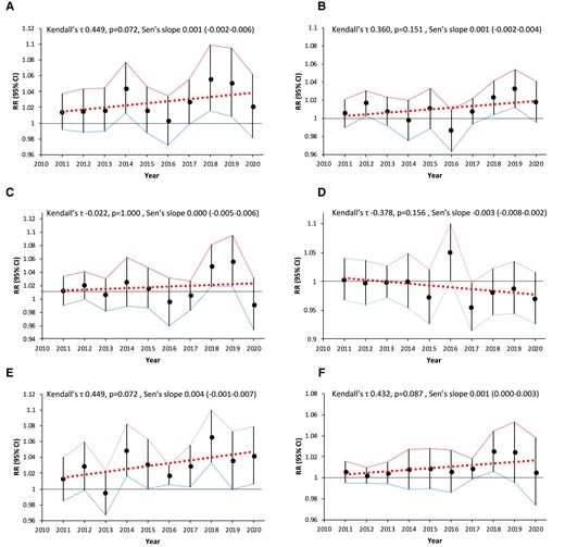
Annual trends of the effects of air pollutants. (A) PM2.5, (B) NO2, (C) CO, (D) O3, (E) B(a)P, and (F) SO2. CI, confidence interval; RR, relative risk.
Acute effects of air pollution
Detailed acute effects of air pollutants on the overall population and in relation to patient and regional characteristics are presented in Figure 3.
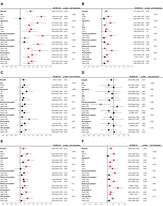
Acute effects of various air pollutants on IS incidence on the day of exposure (LAG 0) in relation to gender, age, alcohol or tobacco consumption, CVD mortality, and AF prevalence. (A) PM2.5, (B) NO2, (C) CO, (D) O3, (E) B(a)P, and (F) SO2. AF, atrial fibrillation; CI, confidence interval; CVD, cardiovascular disease; Q, quartile; RR, relative risk.
In the overall population, exposure to PM2.5, NO2, B(a)P, and SO2 was correlated with increased risk of IS onset on the day of exposure by 2.4% (RR 1.024, 95% CI 1.015–1.032, P < 0.001), 1% (RR 1.01, 95% CI 1.004–1.015, P < 0.001), 0.8% (RR 1.008, 95% CI 1.001–1.016, P = 0.03), and 0.6% (RR 1.006, 95% CI 1.003–1.009, P = 0.001), respectively. More pronounced effects of the exposure to PM2.5, NO2, and B(a)P were noted in non-elderly individuals (all Pinteraction < 0.001). Women were more vulnerable to exposure to PM2.5, NO2, B(a)P, and SO2 than men (all Pinteraction < 0.001).
There was stronger association between exposure to PM2.5 (Pinteraction < 0.001) and SO2 (Pinteraction = 0.025) and IS incidence in inhabitants of regions with high tobacco consumption. Similar effects in the region with high alcohol consumption were noted for PM2.5 (Pinteraction < 0.001), NO2 (Pinteraction = 0.007), and SO2 (Pinteraction < 0.007). There was a correlation between the increased four abovementioned air pollutant concentrations and the IS onset risk in low AF prevalence areas [PM2.5 increased risk of IS onset by 2.8% (RR 1.028, 95% CI 1.016–1.04, P < 0.001)], whereas only PM2.5 (RR 1.019, 95% CI 1.007–1.031, P = 0.002) and SO2 (RR 1.005, 95% CI 1–1.01, P = 0.037) had the same negative effect in high AF prevalence areas.
Similar results were noted regarding the regional differences based on CVD mortality prevalence, although inhabitants of areas with lower CVD mortality were more sensitive to the effects of B(a)P (Pinteraction = 0.023). Exposure to most of the analysed air pollutants was correlated with increased IS risk in the rural territories and counties with lower population density (Figure 3).
Exposure–response function
The exposure–response associations of selected air pollutant concentrations with IS incidence were positive, and the curves showed an increase (Figure 4). The slopes were non-linear and steeper at lower concentrations [for PM2.5 lower than 20 μg/m3, for NO2 lower than 10 μg/m3, for B(a)P lower than 1 μg/m3, and SO2 lower than 2 μg/m3]. At higher concentrations, the slopes flatten, especially in the case of NO2 and SO2.
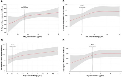
Exposure–response curves. (A) PM2.5. (B) NO2. (C) B(a)P. (D) SO2.
Effects of air pollution according to World Health Organization guidelines
Analyses based on the days with and without exceeding levels of air pollution according to World Health Organization (WHO) guidelines are presented in Figure 5.
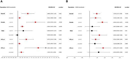
The impact of (A) PM2.5 and (B) NO2 divided into days with non-exceeded and exceeded concentrations according to the WHO guidelines. CI, confidence interval; RR, relative risk; WHO, World Health Organization; y.o, years old.
Exposure to two main air pollutants, PM2.5 and NO2, was associated with increased risk of IS onset on days with exceeded concentrations according to WHO guidelines by 1.6% (PM2.5: RR 1.016, 95% CI 1.006–1.026, P = 0.001; NO2: RR 1.016, 95% CI 1.002–1.03, P = 0.028) and without exceeded levels of air pollution according to WHO norms by 8.8 and 1.9%, respectively (PM2.5: RR 1.088, 95% CI 1.034–1.145, P = 0.001; NO2: RR 1.019, 95% CI 1.01–1.028, P < 0.001).
Similar effects were noticed in females considering the effect of PM2.5 (non-exceeded: RR 1.156, 95% CI 1.076–1.241, P < 0.001; exceeded: RR 1.039, 95% CI 1.025–1.053, P < 0.001), while NO2 had a negative correlation only on days where it had non-exceeded concentrations, increasing risk of IS onset by 3.4% (RR 1.034, 95% CI 1.022–1.047, P < 0.001). Men were affected only on days with exceeded levels of NO2 (RR 1.026, 95% CI 1.006–1.046, P = 0.01) whereas there was no significant association between exposure to PM2.5 and IS incidence on the male population regardless of concentration. Exposure to PM2.5 was negatively correlated with risk of IS onset both on days with exceeding and non-exceeding concentrations according to WHO standards, irrespective of the patients’ age. Contrary to NO2, where both analysed age groups were affected only on days with non-exceeded levels of air pollutants (<65 years old: RR 1.036, 95% CI 1.017–1.056, P < 0.001; >65 years old: RR 1.016, 95% CI 1.006–1.026, P = 0.002).
Results presenting the association between exposure to air pollution and IS incidence not only up to 6 days after exposure but also 0–6- and 0–30-day moving averages are available in Supplementary material online, Tables S7–S12. The results show a lingering harmful effect of air pollution in the days following exposure.
Discussion
The major findings of our study are as follows: (i) air pollution is associated with an increased risk of IS onset on the day of exposure; (ii) effects of air pollution varied between different patient subgroups (age, sex at birth, and lifestyle) and area settings; (iii) exposure to even low levels of air pollutants could have a harmful effect; and (iv) harmful lifestyle (high tobacco and alcohol consumption) might further increase the negative effects of air pollution. Hence, we provide new evidence on the associations between short-term exposure to smog and the risk of IS hospitalization in a region with a relatively low level of air pollution compared to most often studied areas.
In our analysis, we found a significant short-term association between exposure to PM2.5, NO2, B(a)P, and SO2 with IS incidence in the overall population. PMs, one of the main components of Polish smog, alongside B(a)P, exhibited the most adverse effects. In recent literature, there is published evidence about the harmful impact of smog as a trigger for cardiovascular events, but these mainly concern myocardial infarction.10,11,16–18 When it comes to the incidence of strokes, most prior scientific papers originate from the Asian region, which differs not only in terms of air pollution levels but also in its chemical composition, entirely distinct from that in Europe or North America. In a meta-analysis by Toubasi and Al-Sayegh,19 nearly 60% of observational studies included were conducted in Asia. Nevertheless, these studies broadly align with our findings, demonstrating the negative effect of the majority of air pollutants in the general population.20,21 On the other hand, European studies show greater heterogeneity, presenting mixed, conflicting results that mainly focus on the long-term impact of air pollution.22 In one study conducted in Ireland, Byrne et al.23 found no overall association between exposure to PMs or NO2 and stroke incidence with significant results observed solely during the winter season. The Aphea-II study revealed no influence of SO2 on the risk of hospitalization due to stroke in five European countries.24 Nevertheless, a Belgian study showed negative effects of NO2 on the incidence of cardiovascular outcomes, including IS.25 Similar results were obtained for PM10 from the Swedish Riksstroke registry that also showed no influence of O3 and NO2.26 In their nationwide analysis of cardiovascular morbidity in Italy, Stafoggia et al.27 reported a significant impact of PMs on IS incidence, but only in very highly developed municipalities.
Finally, Jiang et al.22 demonstrated varying susceptibility to air pollution depending on genetic predispositions. In summary, the results of environmental studies may slightly differ from each other, although most of them show negative effects of air pollution. The differences in effects may be due to different types of analysed smog (e.g. Polish smog and London smog), differing methodologies or variations in the studied populations (e.g. different genetic predispositions) across individual studies.
Our preliminary results in previous studies suggested that short-term exposure to PMs and NO2 might increase IS morbidity and mortality.6,7 In our current analysis, the exposure–response curves were steeper at lower concentrations and flattened at higher levels of air pollution, similar to those that have been published.20,27 Such exposure–response relationship curves in environmental studies are pivotal for assessing the benefits of air pollution concentration-reducing policies, suggesting that there is no ‘safe’ level of air pollution.
The analysis shows that air pollution effects on IS depends on the patient’s characteristics with the most sensitive groups being females and people under 65 years old. Considering sex differences, available research agrees with our findings.6,28 However, Colais et al.29 argue that sex-related variations in vulnerability depend on the type of disease, presenting women as more sensitive to the onset of heart failure and men to arrhythmias and conduction disorders, while Argacha et al.30 found a stronger association between exposure to air pollution and increased ST-elevation myocardial infarction incidence in males. Studies suggest anatomical, physiological, molecular and socioeconomic differences between two sexes, which might partially explain this phenomenon. First, according to experimental study, there is a greater deposition of particles in the proximal airways in females, which could result in higher dose of air pollutants inhaled among women.31 Second, females might have more potent inflammatory reactions caused by similar doses of air pollution.32 Third, even in highly developed countries, differences in socioeconomic status between both sexes still persist, as the greater sensitivity of women might be attributed to their lower socioeconomic status in the analysed country.33 Finally, behaviour patterns also differ between the sexes, directly affecting the duration and intensity of exposure to air pollution, which can also influence the outcomes.34
Our results are in contrast to published studies, which show that elderly individuals were more vulnerable to air pollution.6,20,21,27,29,35 In contrary, researchers in Chongqing, China, found people under 60 years were more sensitive to O3.36 Yitshak Sade et al.14 reported a higher risk of IS among young adults exposed to PMs in Israel in the years 2005–12. On the other hand, study using data from the Israeli National Stroke Registry between 2014 and 2018 found greater associations between short-term exposure to PM2.5 and IS incidence in elderly individuals.37 These differences could be related to the composition of particles, since the first study was conducted in the southern part of Israel, which is a semi-arid region, with natural dust being a primary contributor to air pollution, while the second analysis encompassed the whole country.14,37 BRICS cohort analysis revealed an exponential increase in CVD mortality and DALYs attributable to air pollution with increasing age among all analysed countries; however, it focused solely on the long-term impact, which differs from our analyses.38 It should be noted that differences in life expectancy exist for reasons unrelated to air pollution, even among neighbouring countries. For example, the analysed country, Poland, has one of the lowest life expectancies in the European Union of 78.6 years compared to 84 years in Spain, which may also impact the results of the analyses.39 The decreasing and increasing incidence of IS among respectively elderly and non-elderly individuals might be linked to better control of classical CVD risk factors and improved treatment of comorbidities, given similar exposure to air pollution, which makes it even more crucial to minimize this significant threat.1 In summary, we hypothesize that the composition of Polish smog may be more harmful in the context of atherothrombotic CVD for non-elderly individuals, as demonstrated by our previous study on myocardial infarction.11 Differences in the socioeconomic status of residents in the analysed countries might affect their age-related vulnerability to air pollution. Moreover, we suggest that this phenomenon might be due to more outdoor activity performed by non-elderly individuals, as increased physical activity in highly polluted areas may have adverse effects on cardiovascular system.40 Exposure misclassification and, most importantly, ‘survival bias’ should also be considered, as elderly people are perhaps more fragile and thus more likely to die in pre-hospital settings, which may lead to underestimation of recorded effects in this specific population. Nevertheless, the recognition of potentially vulnerable patient subgroups in different regions is important for public health objectives since it might help target populations that should minimize individual exposure to smog.
In our analysis, the modifying variables influencing the effects of individual air pollutants were tobacco or alcohol consumption rates, density of population, and CVD mortality, whereas the municipality’s type and AF prevalence did not significantly affect results. Indeed, there are mixed results on smoking and drinking alcohol increasing the negative effects of exposure to smog.41–43 Experimental studies suggest that smoking might lead to inflammation, alveolar injury, and finally, increased alveolar–capillary permeability, which might increase the penetrability of smog particles to the circulatory system.44 Also, Mortensen et al.45 demonstrated that lung mucociliary clearance was faster among lifelong non-smokers in comparison to ex-smokers. These lifestyle behaviours could be also associated with lower socioeconomic status, which might also affect the results, as higher disadvantaged area inhabitants appear more sensitive to air pollution.46,47In vivo studies also show the synergistic or additive influence of smoking on air pollution’s negative effects.21,42,48 This underscores that combating air pollution should be multifaceted and not solely focused on reducing its concentration.
Besides patients’ lifestyle habits, the municipality’s CVD mortality rates play a substantial role in modifying the impact of air pollution. To date, there are no prior studies analysing this relationship. First, observational studies assessing the risk of hospitalization due to CVD may be subject to the ‘survival bias’ mentioned above, whereby high CVD mortality translates into a higher risk of death before reaching the hospital, leading to an underestimation of the effects in these studies. Second, areas with high CVD mortality are characterized by low socioeconomic status, resulting in poorer access to healthcare and less effective primary and secondary prevention of cardiovascular events. Additionally, air pollution can have a direct impact on the incidence of IS, as well as an indirect influence on subsequent coronary events as part of the so-called ‘stroke–heart syndrome’.49 The character of the municipality (urban or rural) did not significantly influence the results in our analysis. In contrast, Zhao et al.50 reported greater sensitivity among rural residents of China, while a study conducted in the southwest region of the same country showed opposite effects.35 On the other hand, Liu et al.51 demonstrated greater effects on CVD mortality in rural areas and higher respiratory mortality in urban areas attributed to PM2.5 exposure. In summary, the results of studies on the impact of air pollution are also influenced by other environmental factors, lifestyle, and socioeconomic variables, which confirm the concept of the ‘exposome’, which refers to the total exposure to environmental factors over a lifetime.52
Personal and systemic measures to minimize exposure to smog and mitigate its negative effects have to be considered, especially in regions with either high concentrations of air pollutants or extremely harmful combinations of air pollution such as Polish smog. First, it is crucial to correctly evaluate patients’ cardiovascular risk; however, current tools fail to incorporate environmental risk factors, such as air pollution. A more precise assessment of CVD risk based also on air pollution exposure might more effectively identify high-risk patients, allowing for earlier implementation of primary prevention. For example, Kim et al.53 demonstrated that the use of statin among people over 60 years old in areas with high levels of PM2.5 and PM10 reduced the risks of stroke by 17 and 21%, respectively. Second, populations, especially those with high-risk patients, should be encouraged to follow air quality forecasts and minimize their exposure to air pollution to an absolute minimum. Finally, and most importantly, systemic changes are necessary to minimize air pollution-related CVD burden. The ‘Air Pollution Prevention and Control Action Plan’ enacted in China in 2013, although costly, yielded highly positive health-related outcomes, particularly for the most socioeconomically disadvantaged groups.54 Also, the European Union with the ‘Zero Pollution Action Plan’ plans to reduce levels of air pollution to levels no longer considered as harmful to society by 2050.55 This allows for coordinated actions among all member countries, such as enaction of stricter emission standards, promotion of sustainable transportation (e.g. electric vehicles and improvement to public transportation), transition towards renewable energy sources to reduce reliance on fossil fuels, and raising public awareness about harmful effects of air pollution. Fight against air pollution is a trade-off battle between the goal of improving quality of life, tied to industrial and social development, and the goal of preserving the environment. In Poland, the primary concern remains outdated heating furnaces and low-quality fossil fuels. Since the main threats to the public health, e.g. tobacco and alcohol, are taxed, one of the implications from our study is the temporary introduction of excise tax on low-quality combustibles and subsidies for exchange of old-type stoves.
Limitations and strengths
To our knowledge, this is one of the largest epidemiological studies examining the association between short-term exposure to various air pollutants and IS incidence conducted in Europe. We have analysed the effects of air pollutants previously overlooked in scientific papers, such as B(a)P. Furthermore, we have used innovative modelling methods of air pollution concentrations (GEM-AQ), which have provided us with an unprecedented level of accuracy. Lastly, we did not solely focus on the direct impacts of smog; rather, we thoroughly examined their effects based on patient characteristics and the aspects of their residential areas in a region that has been inadequately studied thus far. Our analysis suggests that avoiding exposure to air pollution is a pivotal aspect of primary IS prevention, and the inclusion and mitigation of epidemiological risk factors in guidelines have to be considered.
Our study has several limitations. First, we utilized residential zip codes to connect individual exposure and IS incidence, which may result in potential misclassifications due to outdated codes and people’s mobility, even though we used the GEM-AQ model to minimize such risk. Second, the nature of our research did not allow us to account for the impact of indoor air pollution, but its contribution in highly developed countries, such as Poland, is marginal.1,3 Third, the analysis of lifestyle was conducted at the NUTS-2 level, as our data sets did not include individual-level data on socioeconomic status and lifestyle habits, which influenced our chosen methodological approach and analysis plan, and therefore may affect the results and potentially lead to an ecological fallacy, where associations observed at the group level may not apply to individuals. Lastly, due to the retrospective and observational cohort design of this study, along with the unavailability of some relevant confounders, causal inference is precluded.
Conclusions
Exposure to air pollution might be associated with higher IS incidence, particularly posing a higher risk to non-elderly women. Harmful lifestyle habits, such as high tobacco and alcohol consumption habits, might exacerbate the negative effects of air pollution. Exposure to even low levels of air pollutants could have a harmful impact with no ‘safe’ levels of air pollution.
Supplementary material
Supplementary material is available at European Journal of Preventive Cardiology.
Acknowledgements
We would like to express our sincere gratitude to the National Health Fund, the Chief Inspectorate of Environmental Protection, the Polish Academy of Sciences, and all EP-PARTICLES investigators. Presented at ESC Preventive Cardiology 2024 in the ‘Young Investigators Award - Population Science and Public Health’ session in Athens, Greece.
Author contribution
Ł.K. contributed to the conception or design of the work. M.Ś., E.J.D., J.W.K., J.S., and Ł.K. contributed to the acquisition, analysis, or interpretation of data for the work. All authors drafted the manuscript. M.Ś., G.Y.H.L., and Ł.K. critically revised the manuscript. All gave final approval and agreed to be accountable for all aspects of work ensuring integrity and accuracy.
Funding
The study was financed from the funds of the National Science Centre, Poland granted under the contract number UMO-2021/41/B/NZ7/03716 and the funds of the Medical University of Bialystok, Poland granted under the contract numbers B.SUB.23.101, B.SUB.24.111, B.SUB.24.560, and B.SUB.23.509. The Medical University of Bialystok, Poland funded the APC. The funders had no role in considering the study design or in the collection, analysis, interpretation of data, writing of the report, or decision to submit the article for publication.
Ethical approval
The study protocol conformed to the ethical guidelines of the 1975 Declaration of Helsinki and was approved by the Bioethics Committee of the Medical University of Bialystok (approval number APK.002.81.2022).
Data availability
Anonymized data might be shared upon reasonable request.
References
Eurostat. EU life expectancy estimated at 81.5 years in 2023. Available online: https://ec.europa.eu/eurostat/web/products-eurostat-news/w/DDN-20240503–2.
Author notes
Conflict of interest: G.Y.H.L: Consultant and speaker for BMS/Pfizer, Boehringer Ingelheim, Daiichi-Sankyo, Anthos. No fees are received personally. He is a National Institute for Health and Care Research (NIHR) Senior Investigator and co-PI of the AFFIRMO project on multimorbidity in AF (grant agreement No 899871), TARGET project on digital twins for personalised management of atrial fibrillation and stroke (grant agreement No 101136244) and ARISTOTELES project on artificial intelligence for management of chronic long term conditions (grant agreement No 101080189), which are all funded by the EU’s Horizon Europe Research & Innovation programme. Other authors declare no conflicts of interest.

Comments