


Abstract
We investigate the link between the 1918 Great Influenza and regional economic growth in Italy, a country in which the measures implemented by public authorities to contain the contagion were limited or ineffective. The pandemic caused 600,000 deaths in Italy: 1.2% of the population. Going from regions with the lowest mortality to those with the highest mortality is associated to a decline in per capita GDP growth of 6.5%, which dissipated within 3 years. Our estimates provide an upper bound of the adverse effect of pandemics on regional economic growth in the absence of non-pharmaceutical public-health interventions.
1. Introduction
The COVID-19 pandemic induced policymakers to take rapid decisions about urgent policy interventions to contain the contagion and its consequences. These decisions were based on weighing the effects of the pandemic and those of the interventions. To cast light on these issues, a renewed interest in the literature on the effects of historical pandemics analyzes the consequences of the 1918–21 Great Influenza, one of the largest pandemics in recent history.
Barro et al. (2020) provide a cross-country study of the effect of the Great Influenza on economic growth and find that a death rate of 2% was associated with a drop in real per capita gross domestic product (GDP) of 6% for the typical country. The institutional and environmental differences across countries, and in their response to the pandemic, motivate also a growing literature on the within-country effects of the influenza. For instance, Correia et al. (2020) offer an analysis across US cities and states, Moller Dahl et al. (2020) explore heterogeneity across Danish municipalities, and Basco et al. (2021) across Spanish provinces. These studies are useful in understanding the economic effects of pandemics in contexts were institutions have the capacity to implement, at least in part, non-pharmaceutical public-health interventions (NPIs), such as lockdowns. However, it is not clear to which extent these estimates are also informative in contexts in where NPIs are adopted too late to be effective or are not adopted at all.
In this paper we study the effects of the 1918 Great Influenza on local economic activity and exploring the different regional exposure to the pandemic in Italy. Similarly to the COVID-19 pandemic, Italy was one of the European countries most severely exposed to the influenza (Johnson & Mueller 2002). Furthermore, the censorship due to the involvement of Italy in the war annihilated the possibility to use the media to implement NPIs. The great exposure of Italy to the influenza, along with the limited or ineffective public health interventions undertaken to contain it, provide the opportunity to estimate the potentially adverse effect of one of the largest pandemics in recent history on local economic growth in the absence or limited NPIs, a condition that several developing countries are facing these days.
The 1918 influenza outbreak caused about 600,000 deaths in Italy, which occurred mostly between end September and early November 1918. Mortality varied substantially across regions ranging from 0.7% in Veneto to 1.7% in Apulia and 1.9% in Campania. We use this variability across regions to investigate the effect of the health shock on subsequent GDP growth. To assess the impact on GDP of the influenza we follow an approach similar to that adopted by Barro et al. (2020) and regress regional GDP growth on flu mortality for various sample periods between 1900 and 1930, and controlling for other potential covariates such as war mortality, initial GDP, proxies for human capital, and regional fixed effects.
Differences in flu mortality rates may be partly explained by different exogenous climatic conditions (Sagripanti & Lytle 2007; Weber & Stilianakis 2008). Other factors, such as initial differences in human capital and economic development, have an independent effect on economic growth, but may also interact with flu mortality. We address these concerns using a flexible econometric specifications, showing that the growth effect of flu mortality arises precisely at the time of the outbreak, but not before. As we shall see, this result suggests that our estimates capture the effect of the flu rather than the effect of other variables, like the level of economic development and human capital, which should affect growth also before the pandemic.
We find that the influenza contributed substantially to the different performance of the Italian regions during the 1919–21 recession. Regions with the highest mortality rates experienced a roughly 6.5% excess decline in GDP relative to regions that experienced the lowest mortality rates. Using a distributed lag specification, we find that the impact of the influenza on regional growth was highest immediately after the pandemic and that the effect vanished within 3 years. We obtain the same results with a difference-in-differences specification as well as with a flexible specification.
We also find that the effect of the pandemic was stronger in more densely populated regions, and with higher share of regional manufacturing employment. These findings support the hypothesis that the pandemic reduced the demand for goods and services, in line with recent findings in the context of Spain (Basco et al. 2021). In the long run (10 years and over), the statistical analysis reveals a small and negative effect of the influenza on industrialization. Overall our results are qualitatively consistent with recent cross-country evidence in Barro et al. (2020), and sub-national evidence for the USA (Correia et al. 2020) and Denmark (Moller Dahl et al. 2020).
From an economic point of view, our results suggest that the reduction in the labor force and the fear of the spread of the pandemic led to a reduction in economic growth. Historical accounts of the influenza pandemic reveal that the response of the health care system was essentially inadequate in all regions and that lockdown measures were mild and ineffective. Therefore results are relevant to analyze the potential impact of epidemics in developing countries with poor health infrastructure and limited ability to impose and enforce lockdown measures. More generally, our paper speaks to the literature studying the effects of epidemics, and their eradication, on economic development and growth.
The paper is organized as follows. In Section 2 we describe the development of the 1918 influenza in Italy and the recession of 1919–21. Section 3 reviews the possible economic mechanisms linking pandemics and economic growth, and the empirical literature on the economic effects of the 1918 influenza. Section 4 describes our data, and Section 5 provides descriptive evidence on the recessionary impact of the pandemic. Section 6 presents our baseline results linking GDP growth and influenza mortality using different specifications and taking into account regional and time fixed effects, as well as regional differences in economic development and human capital. Section 7 explores heterogeneous effects and the potential effects of the pandemic on industrial development. Section 8 summarizes our main findings.
2. The 1918 Influenza in Italy
The 1918 influenza killed at least 40 million people worldwide (possibly many more), corresponding to 2 percent of the world’s population at the time. Italy was one the most severely affected countries. Current estimates suggest that about 0.6 million out of 36 million people died similar to the number of military deaths in WWI, at an estimated mortality rate of 1.2%, below the world average but substantially above the mortality rates of other developed countries (Barro et al. 2020). For instance, in Germany, the estimated mortality rate was 0.8%, in the USA and the UK it was 0.5%, and in France it was 0.7%. So, the combined effect of influenza and war mortality reduced a population of 36 million by about 1.2 million between 1915 and 1918.
There were two waves of the influenza between May 1918 and early 1919. The first wave in Spring 1918 was relatively mild but the second wave was severe. The first infections were reported in late August and by mid-September the influenza had spread to all parts of Italy, reaching a peak in early to mid-October and ending mostly in November but with some cases still being registered in January and early February 1919. The influenza hit all parts of Italy very quickly. Tognotti (2015) provides a thorough investigation of the pandemic and reports that deaths peaked in mid-October with only around a couple of weeks lag between it spread to the different regions of the country.1
Several factors contributed to the spread of the disease and the high mortality rate. First, the spread of the influence coincided with the end of WWI, the last Italian attack against the Austro-Hungarians in late October, and the final victory on November 4, 1918. The movements of troops, sick soldiers, and refugees in both Southern and Northern Italy most likely contributed to the rapid spread of the disease. While in many countries, social distancing and quarantine measures were implemented, in Italy the lack of coordination and poor organization meant that these measures were implemented too late to stop the pandemic and were largely ineffective.
The material conditions of the Italian population were another aggravating factor. Cohabitation of entire families in the same room, overcrowding, and lack of running water, electricity, toilets, and sewers were the rule rather than the exception in many parts of Italy, with most people living in precarious conditions. Although we have no systematic accounts of social distancing measures that can be exploited in the empirical analysis of the economic impact of the pandemics, Tognotti (2015) reports that these measures were introduced only when the pandemic was out of control, and in practice were futile or unfeasible.2
The information provided by the press was limited due to the initial censorship in place to ensure that the enemy did not receive news about the real proportion of the epidemic. Furthermore, healthcare was also problematic since most doctors and medical personnel had been diverted to support the military, and hospitals existed only in large cities and not smaller towns and rural areas. The limited ability to use the media to contain the contagion, along with the inadequate healthcare support, make the flu pandemic in Italy an important historical event to cast light on the effects of pandemics in contexts where institutions have limited capacity to hinder the spread of the infection.
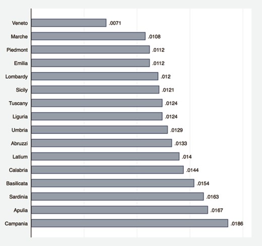
As in other countries, mortality was highest among the young (20 to 40 year old) but the Italian case is peculiar for its sizable mortality of young women. Pinnelli & Mancini (1998) proposed the explanation that since contagion depends on frequency of contact, girls were more likely to succumb because of their higher exposure to the flu based on their care of the elderly and sick. Mortality also varied considerably across regions, exceeding 1.5% in regions such as Campania and Apulia, whereas in others such as Veneto it was substantially less than 1% (see figure 1 and table B.2 in Appendix B.). To some extent, these differences likely reflect resources, human capital, and infrastructure gaps between the North and South of the country. Therefore, when assessing the economic consequences of epidemics, it is important to take account pre-existing differences in initial conditions.
Flu mortality by region
We measure regional flu mortality by using official flu mortality statistics. An alternative approach would be to estimate excess mortality in the year of the pandemic relative to other years. Mortality measures based on official statistics have some limitations, such as non-registration, missing records, and misdiagnosis, which may potentially underestimate mortality (Johnson & Mueller 2002). Nevertheless, besides simplicity and transparency, they have two important advantages in our context. First, they are unaffected by the choice of a reference period: a particularly complex choice in the context of Italy, given that the year of the pandemic outbreak was the last year of WWI. Second, they are not affected by excess mortality due to the war and its associated hardships.
Reassuringly for our empirical analysis, the Italian national official flu mortality rate (1.1%) is quite close to the recalculated death rate based on the excess mortality approach (1.07%) (Johnson & Mueller 2002, p.113, table 4), suggesting that the official statistics are a valid measure of flu mortality, at least in the Italian context. See Appendix B for additional details on the reliability of the mortality statistics used in this paper.
It should be noted also, that ideally, to assess the overall effect of the exposure to the influenza pandemic both contagion and mortality should be considered. Nevertheless, to the extent that contagion is proportional to mortality, our estimates include the overall effect of exposure to the disease.
The pandemic hit the Italian economy in the last year of WWI, a period of significant economic expansion particularly of firms involved in war production stimulated by large government expenditures. The war was followed by a recession in 1919–21, which saw a large fall in per capita GDP in 1919 (-19%) and a cumulative decline of approximately 30% over the 3 years. In this paper we focus on the specific role of the 1918 influenza in explaining regional economic growth during the recession.3
3. The economic impact of pandemics
The literature on the economic consequences of the 1918 influenza points to a variety of mechanisms at work, even only focusing on short-run growth effects, which is the object of this paper. On the supply side, one possible effect is directly induced by mortality, which shrinks the labor force and increases the ratio of capital and land to labor. This supply-side force should increase the wage rate and reduce the returns to capital and land, slowing investment and capital accumulation. On the demand side, pandemics are associated with fear of contagion, loss of confidence, and increased uncertainty, in turn seriously disrupting economic activity via a reduction in the demand for goods and services, causing high unemployment and low wages. Although they have different implications for factor prices, both these forces would lead to an adverse effect of the pandemic on economic growth.
The recession could also have long-run consequences because human capital (in the form of both health and education) falls during and after a pandemic, reducing labor productivity especially in higher human capital-intensive sectors (manufacturing). Human capital externalities might affect the productivity of other workers, and of the economy at large. Thus, the reduction in savings might be exacerbated by lower investment in human capital, for instance in children’s education and the health infrastructure.4
While most economic arguments lead to the presumption that pandemics have recessionary effects, empirical analyses provide different estimates for size and duration of the effect. The typical empirical approach is to study variations in flu mortality rates across countries, regions, or cities and to trace the effect of the pandemic on various outcomes (GDP or GDP components, wages, poverty rates, and human capital levels) in the years (or decades in some studies) after 1918.
In assessing the literature on the economic effects of the 1918 pandemic in the USA, Garrett (2008) concludes that most of the evidence indicates that the effects were short lived, hitting firms and households differentially. According to Garrett (2009), the most noticeable effect of the pandemic was to decrease the manufacturing labor supply and increase wages growth in US states and cities by 2 to 3 percentage points for a 10 percent change in per capita mortality.
Brainerd & Siegler (2003) found that the 1918 epidemic was positively correlated to subsequent economic growth in the USA. In particular, one additional death per thousand resulted in an average annual increase of 0.15% per year in the rate of growth of real per capita income over the following 10 years. The authors argue that after the pandemic states with higher flu mortality rates showed a higher increase in capital per worker, and thus also income per worker.
Basco et al. (2021) explore the effect of the flu pandemic across Spanish provinces. They found that in Spain aggregate output and consumption were only mildly affected, but that there was a large, negative, and short-lived effect on wages, especially in highly urbanized areas and in occupations producing non-essential goods. Their findings suggest that the influenza induced a negative demand shock that was mostly absorbed by workers.
Correia et al. (2020) used geographic variation in mortality during the 1918 influenza outbreak in the USA and found that more exposed areas experienced a sharp and persistent decline in economic activity. In particular, they found that the influenza epidemic led to an 18% reduction in state manufacturing output for states at the mean level of exposure. They use variation in the degree and intensity of non-pharmaceutical interventions (lockdown) and found that cities that intervened earlier and more aggressively performed no worse, and if anything, grew faster after the epidemic.5
The Swedish and Danish cases are interesting because neither country was involved in WWI, which reduces the risk of the pandemic’s effects being confounded by disturbances related to the war. However, both countries suffered the indirect effects of the war on international trade. Karlsson et al. (2014) show that in Sweden the pandemic had a strong negative impact on capital income: the highest quartile (with respect to influenza mortality) experienced a drop of 5% during the pandemic and an additional 6% afterwards. The pandemic also increased the poverty rate (defined as the share of the population living in public poorhouses) but had no effect on earnings. Moller Dahl et al. (2020) find that more severely affected Danish municipalities experienced short- run declines in income (5% between 1917 and 1918), suggesting that the epidemic led to a V-shaped recession with relatively moderate, negative effects in the shortrun and a full recovery after 2–3 years. They also report that unemployment rates were high during the epidemic but decreased only a couple of months after it declined. It should be noted also that overall, Denmark experienced one of the lowest mortality rates worldwide (Barro et al. 2020), 0.3% against a world average of 2%.
Barro et al. (2020) provide an overall assessment of the effect of epidemics in a cross-country comparative study. They regress the annual growth rate of per capita GDP between 1901 and 1929 against the current and lagged values of the flu death rate and the war death rate for a panel of 42 countries. They find a flu death rate coefficient of -3.0 meaning that, at the cumulative aggregate death rate of 2% for 1918–1921, the epidemic is estimated to have reduced real per capita GDP by 6% for the typical country.6
There is also an important stream of work on the economic consequences of pandemics in Italian history. For instance, Alfani (2013) emphasizes that as 17th century plagues in Europe had more severe effects on Italy and Southern Europe generally, they hindered the economic performance of Italy relative to Northern European countries. Alfani & Percoco (2019) explore the effects of plagues for Italian cities in pre-industrial times. They show that the 1629–30 plague was linked to persistently lower economic growth in cities more exposed to the infection. Malanima (2018) points to the effect of the severe and frequent plagues that affected the Italian peninsula during the Renaissance (1350–1550) and shows that they were associated to an increase in resources per worker, and ultimately improving living standards, which eventually converged to their low pre-Renaissance levels. Our study contributes to this strand of work by exploring the Great Influenza Epidemic, which affected the Italian economy in a more recent historical period, and focusing on regional rather than aggregate economic growth.
Finally, our paper speaks to the literature studying the effects of epidemics, and their eradication, on economic development and growth.7Cervellati & Sunde (2015) build a model in which mortality differences induce differences in the timing of the transition from Malthusian stagnation to modern economic growth, which is a key determinant of current differences in living standards (Galor 2011). In a similar framework, Lagerlöf (2003) develops a model in which the frequency of epidemics induces parents to invest in the quantity of children rather than in their education, delaying the timing of the escape from the Malthusian trap. Corrigan et al. (2005) build an OLG model where an AIDS epidemic reduces human capital accumulation and growth through the creation of large numbers of orphans. While some works explain long-term economic development across European localities with the differential exposure to the Black Death (Pamuk 2007; Voigtländer & Voth 2013), other empirical papers employ data across countries to explore the epidemiological transition and its effects on life expectancy, population, and education (Acemoglu & Johnson 2007; Klasing & Milionis 2020). Hansen (2014) uses data across US localities to empirically show that medical innovations had significant positive effects on life expectancy, population, and GDP. By studying a country with limited health infrastructures and capacity to adopt non-pharmaceutical public health interventions, the present paper complements the literature emphasizing that health and other large economic shocks may have non-monotonic effects over the development process (Cervellati & Sunde 2011; Noy 2009).
4. Data
We use yearly data on real GDP per capita provided by Daniele & Malanima (2011) for the 16 Italian regions in 1918.8 We link GDP data to information on influenza mortality from the 1918 Mortality Statistics Volume (Statistica delle Cause di Morte 1918) compiled by the Ministry of the National Economy (see Appendix B), which we digitized. These data provide information on causes of deaths. We measure deaths due to the Great Influenza by summing the deaths for flu, penumonia, and bronchopneumonia (specifically we sum influenza, broncopolmonite, and polmonite). We construct the mortality variable by dividing the number of regional deaths from these diseases in 1918 by the population according to the 1911 Italian Statistical Office Population Census. Data for 1918 include most deaths from influenza. Our baseline estimates do not include data on influenza in 1919, but the robustness checks include 1919 deaths from influenza and pneumonia in the 1918 cases since these deaths occurred mostly in January and early February 1919.
We also digitized the number of deaths due to WWI from the Albo d’Oro archive of the Institute for History and Resistance and Contemporary Society (Istoreco). Year of death often is uncertain because of late recording and lagged military deaths due to wounds. Thus, our variable for WWI death rates refers to the total number of military deaths during WWI in the 1911 population during the years when Italy was involved in the conflict (1915–1918) and is zero for the other years. For our long-run analysis, as outcome we use the regional share of the labor force employed in manufacturing taken from Daniele & Malanima (2014a). Appendix B provides further details on the variables definitions and sources.
5. Descriptive evidence
Before presenting the regression analysis, it is useful to report the correlations among flu mortality, GDP, and human capital indicators in the pre-war period. Table 1 reports coefficient estimates from regressing per capita GDP in 1913, the share of manufacturing employment in 1911, the WWI death rate, 1911 literacy, and the 1911 Human Development Indicator, against the regional mortality rate due to the 1918 influenza. The evidence does not support the hypothesis that flu mortality was higher in regions that before the war exhibited lower incomes (either in 1910–14 or just in 1913) and a lower share of labor employed in manufacturing. Indeed, the standard errors (square brackets in table 1) indicate that the correlations are not statistically different from zero.
Flu mortality and pre-1918 characteristics
| (1) | (2) | (3) | (4) | (5) | (6) | |
| Dependent variables: | ||||||
| Ln GDP pc | Ln GDP pc | % Manuf. L.F. | WWI | Literacy | HDI | |
| Avg 1910-14 | 1913 | 1911 | death rate | 1911 | 1911 | |
| Flu mortality | -6.482 | -7.753 | -4.069 | -0.332** | -40.349*** | -36.143*** |
| [14.833] | [14.461] | [4.177] | [0.119] | [10.701] | [8.647] | |
| Observations | 16 | 16 | 16 | 16 | 16 | 16 |
| R-squared | 0.007 | 0.010 | 0.030 | 0.091 | 0.336 | 0.382 |
Notes: The regressions are estimated on cross-sectional data. Robust standard errors are reported in brackets. ***indicates significance at the 1% level, **indicates significance at the 5% level, *indicates significance at the 10% level.
Table 1 and figure 2 indicate that influenza mortality was lower in regions that suffered a high WWI death rate (the regression coefficient is -0.33 and statistically different from zero at the 5% level). For instance, Veneto has the lowest flu mortality but one of the highest WWI death rates; the central regions of Emilia, Marche, and Tuscany exhibit relatively high war death rates but below average flu mortality. As we shall see, in our regression analysis, the negative correlation between the two mortality rates helps to distinguish the separate effects of war and flu mortality on subsequent GDP growth. Table 1 shows also that flu mortality is correlated negatively with literacy and the Human Development Index, as suggested also in Tognotti’s (2015) historical account of the pandemic. Therefore, it is important in the empirical analysis to control for measures of human capital.
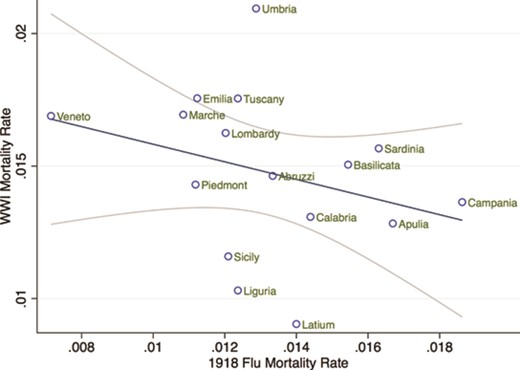
Flu mortality and WWI mortality
Figure 2 provides a first graphical analysis of the relation between the flu death rate and GDP growth rate in 1919–24. During this period, average growth was negative, reflecting the 1919–21 recession. However, regions with above average flu mortality (such as Calabria, Campania, and Latium) exhibit lower than average growth, while regions with more limited mortality (Veneto and Marche) suffered a milder recession. Overall, figure 3 shows that a doubling of the flu death rate (e.g. from 0.8% in Veneto to 1.6% in Sardinia and Apulia) is associated to a 1% reduction in subsequent annual growth.
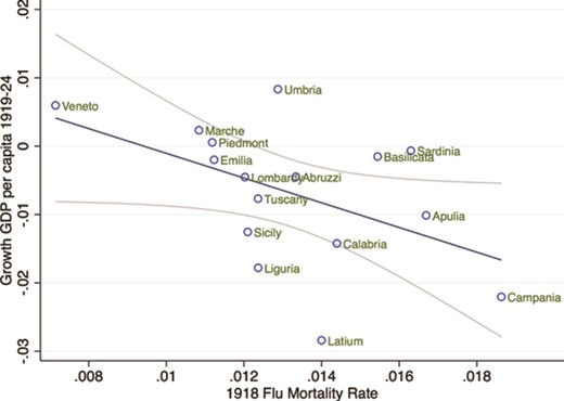
Economic growth and 1918 flu mortality
6. Regression analysis
In this section, we explore through regression analysis the link between influenza mortality and regional growth. Our analysis proceeds in two steps. In Section 6.1 we present our main findings of the link between flu mortality and economic growth using a distributed lag model. This approach extracts in a simple and compact way the main correlations present in the data. In Section 6.2 we generalize the model using a more flexible approach, which removes and tests some of the assumptions we maintain in Section 6.1, and particularly the absence pre-pandemic differential trends and their interactions with local economic development, human capital, and other control variables.
6.1. Distributed lag specification
where |$y_{it}$| is GDP growth in region |$i$| at time |$t$|, |$\gamma _i$| is a set of regional fixed effects, |$\beta _{s}$| is the set of the estimated coefficients, |${\boldsymbol {X}}$| is a matrix of control variables that vary depending on the specification, and |${\boldsymbol {\phi }}$| is the associated vector of estimated coefficients. Finally, |$\epsilon _{it}$| is the error term. For |$s=0$|, the estimated coefficient, |$\beta _{0}$|, represents the association between 1918 flu mortality and economic growth in that same year, conditioning on its lagged effects. For |$s>0$|, the coefficients |$\beta _{s}$| estimate the link between flu mortality in 1918 and economic growth in later periods, conditioning on contemporaneous effect and all other lags.9
Table 2 presents a specification in which we restrict the sample of real per capita GDP growth to the years from 1919 to 1924 to capture the short-run effects of the pandemic and minimize concerns about the difficulty related to introducing WWI period data in the regression. Our variable of interest is influenza mortality in 1918 lagged 1 year. Later, we extend the analysis by introducing more lags and a more flexible specification. We correct the inference by clustering standards errors at the region level to allow serial correlation of the error terms across periods.
Flu mortality and growth in GDP per capita 1919–1924
| (1) | (2) | (3) | (4) | |
| Flu mortality—1 year lag | -13.371*** | -10.841*** | -10.492*** | -11.440*** |
| [0.695] | [2.556] | [2.282] | [2.613] | |
| Flu mortality—2 years lag | -7.904*** | |||
| [2.373] | ||||
| Flu mortality—3 years lag | -1.927** | |||
| [0.846] | ||||
| Flu mortality—4 years lag | -0.485 | |||
| [0.526] | ||||
| WWI death rate 1918 | -2.402 | -2.749 | -3.334*** | |
| [2.173] | [1.944] | [0.888] | ||
| Observations | 96 | 96 | 96 | 96 |
| R-squared | 0.626 | 0.629 | 0.638 | 0.901 |
| Initial GDP per capita | No | No | Yes | Yes |
| WWI death rate lags | No | No | No | Yes |
Notes: The regressions are estimated on a regional panel data for 1919–1924. The dependent variable is the growth of per capita GDP. Robust standard errors clustered at the regional level are reported in brackets. ***indicates significance at the 1% level, **indicates significance at the 5% level, *indicates significance at the 10% level.
In column 1, the coefficient of flu mortality is -13.37 and is statistically different from zero at the 1% level. In terms of economic significance, comparing regions with relatively high and low mortality rates, going from Marche or Piedmont that display rates of about 1%, to Calabria or Basilicata that both have mortality rates of about 1.5%, is associated to a reduction in GDP growth of 6.5%.
These effects are broadly comparable in magnitude to Barro et al.’s (2020) around 6% estimated for a cross-country setting. Our coefficient is slightly larger, possibly because interventions implemented by central and local authorities to limit the spread of the pandemics were weak or ineffective.
The regression of column 2 of table 2 controls for WWI mortality, i.e. the total number of military deaths during WWI over the 1911 population. The variable is built in a similar fashion to our variable of interest: it takes the value zero for the years after 1918 and is lagged 1 year. While the estimated coefficient of WWI mortality is negative but not statistically different from zero, the coefficient of flu mortality remains negative, statistically significant, and almost the same as the regression reported in column 1. The difference between the size of the two coefficients reflect the fact that flu mortality is correlated with contagion and fear of contagion, which may magnify the effect of flu deaths on growth.
To take account pre-existing differences in levels of economic activity, column 3 controls for initial GDP per capita which refers to the initial year of the sample. This additional control has almost no effect on our coefficient of interest whose magnitude and statistical significance are almost unchanged. In the following, we will show robustness to including additional pre-pandemic control variables. Since the effect of the influenza on economic growth could have extended over more than a single year, in column 4 we introduce four lags of flu mortality. As a control, we also introduce four lags for WWI mortality (coefficients not reported in table 2). The coefficients of the lagged influenza variables are negative and significant up to the third lag, implying that the adverse effect of the pandemic on economic growth lasted for 3 years. This finding suggests that the effect of the Italian pandemic on regional economic growth was transitory, which is consistent with recent findings for the effect of the 1918 influenza across Danish municipalities (Moller Dahl et al. 2020).
Table 3 extends the sample to 1929. We do not go beyond 1929 to avoid the confounding effect of the 1930s Great Depression. It can be seen that the estimated coefficients are very similar in magnitude and significance to those in table 2. This further supports the conclusion that the adverse effects of the pandemic on growth were transitory.
Flu mortality and growth of GDP per capita, 1919–1929
| (1) | (2) | (3) | (4) | |
| Flu mortality—1 year lag | -13.771*** | -11.038*** | -10.868*** | -11.227*** |
| [0.742] | [2.606] | [2.449] | [2.599] | |
| Flu mortality—2 years lag | -7.692*** | |||
| [2.415] | ||||
| Flu mortality—3 years lag | -1.714** | |||
| [0.670] | ||||
| Flu mortality—4 years lag | -0.273 | |||
| [0.422] | ||||
| WWI death rate 1918 | -2.582 | -2.750 | -3.334*** | |
| [2.186] | [2.053] | [0.867] | ||
| Observations | 176 | 176 | 176 | 176 |
| R-squared | 0.520 | 0.523 | 0.526 | 0.714 |
| Initial GDP pc | No | No | Yes | Yes |
| WWI death rate lags | No | No | No | Yes |
Notes: The regressions are estimated on a regional panel data for 1919–1929. The dependent variable is the growth of per capita GDP. Robust standard errors clustered at the regional level are reported in brackets. ***indicates significance at the 1% level, **indicates significance at the 5% level, *indicates significance at the 10% level.
Table 4 extends the sample backwards and includes the entire period 1901–1929. This longer sample allows us to include contemporaneous flu mortality and lags up to the fourth year. The estimated coefficient of the contemporary effect in column 1 is positive and precisely estimated, but very small in magnitude. The positive sign of the coefficient may be explained by the fact that it refers to 1918, the last year of the war, which may potentially confound the estimate. Indeed, as we shall see, by introducing in the regression WWI casualties the coefficient of flu mortality turns out to be negative even in 1918. The coefficients of lagged flu mortality are negative and highly significant up to the third lag, in line with our previous findings. The coefficient of the fourth lag is positive and significant. However, this coefficient is not robust across specifications, thus we cannot reject the hypothesis that the influenza had a persistent effect on the level of economic development.
Flu mortality and growth in GDP per capita 1901–1929
| (1) | (2) | (3) | (4) | (5) | |
| Flu mortality | 0.586*** | -0.210 | -0.305 | -0.230 | -0.104 |
| [0.153] | [0.489] | [0.531] | [0.555] | [0.719] | |
| Flu mortality—1 year lag | -15.555*** | -13.392*** | -13.565*** | -13.619*** | -13.390*** |
| [0.886] | [1.682] | [1.767] | [1.805] | [2.113] | |
| Flu mortality—2 years lag | -8.474*** | -4.857** | -5.031** | -4.985** | -4.756* |
| [0.917] | [1.869] | [1.977] | [2.014] | [2.293] | |
| Flu mortality—3 years lag | -3.555*** | -3.805*** | -3.978*** | -3.824*** | -3.595** |
| [0.221] | [1.103] | [1.167] | [1.179] | [1.496] | |
| Flu mortality—4 years lag | 1.324*** | -0.410 | -0.505 | -0.298 | -0.172 |
| [0.243] | [0.944] | [0.994] | [0.965] | [1.123] | |
| Observations | 464 | 464 | 464 | 464 | 464 |
| R-squared | 0.562 | 0.715 | 0.718 | 0.726 | 0.726 |
| WWI death rate | No | Yes | Yes | Yes | Yes |
| Initial GDP per capita | No | No | Yes | Yes | - |
| Time trend | No | No | No | Yes | Yes |
| Region FE | No | No | No | No | Yes |
Notes: The regressions are estimated on a regional panel data for 1901–1929. The dependent variable is the growth of per capita GDP. Robust standard errors clustered at the regional level are reported in brackets. ***indicates significance at the 1% level, **indicates significance at the 5% level, *indicates significance at the 10% level.
Table 4 column 2 includes the contemporaneous WWI death rate, and its lags up to four years. As mentioned, the contemporaneous effect turns negative when introducing this control, in turn suggesting that the potential confounding effect of WWI exposure may induce a bias with the opposite sign to the effect of flu mortality. The estimated coefficients of flu mortality lags are negative and significant up to the third lag. In column 3, we control for the initial level of per capita GDP. It is reassuring that the introduction of this control leads to only minor changes in the estimated coefficients. Column 4 accounts for potential common trends with the inclusion in the regression of a time polynomial of order 2. The results essentially remain unchanged, reducing concerns about the possible confounding effect of a common trend across regions. In Section 6.2 we will further strengthen this result by taking into account a full set of year fixed effects.
In column 5, we test the robustness of our results introducing regional (our geographical unit of analysis) fixed effects to control for heterogeneity in initial region specific conditions.10 Remarkably, the estimates are robust to the introduction of fixed effects that absorb all regional (and time-invariant) differences in human capital, health status, population structure, and growth rates during and before WWI. Also, they control for specialization patterns across regions not captured by initial GDP. For instance, they control for differences between the North-West, which specialized in heavy industries, and the South, which specialized in agriculture.11
Overall, the regression results presented in this section point to a strong and negative association between flu mortality and economic growth, an effect that was absorbed within 4 years from the pandemic.
6.2. Flexible specification
Results so far rest upon the assumption that the determinants of regional differences in flu mortality did not have an independent effect on regional economic growth in the years of the flu pandemic. A formal test in support of the validity of this assumption is to show that, prior to the pandemic, flu mortality was not statistically associated with economic growth. This evidence would suggest that whatever caused differential exposure to the flu, it became salient only in the pandemic period but not before, in turn providing strong support to our identification assumption.
where |$y_{it}$| is per-capita GDP growth in region |$i$| in year |$t$|, |$\gamma _i$| is a set of region fixed effects, and |$\delta _t$| is a set of time fixed effects. Our variable of interest, |$flu_{i,1918}$|, is the same mortality rate used in the regressions of Section 6.1, but it is now constant over time. However, we can still estimate the coefficients indicating the effect of mortality in each year (the set of |$ \beta _{t}$|), by interacting |$flu_{i,1918}$| with the time fixed effects. Each |$ \beta _{t}$| can be interpreted as the excess average regional growth rate in year |$t$| due to flu mortality, relative to the initial year of the sample. We also interact each of the control variables in |${\boldsymbol {X}}$| with time indicators to take into account the time-varying effects of time-invariant characteristics. Finally, |$\epsilon _{it}$|, is the error term of the equation.
Prior to the pandemic, there is no reason to believe that regions more exposed to the flu were systematically growing at a slower speed. Thus, we would expect the estimated |$ \beta _{t}$| coefficients to be statistically indistinguishable from zero before 1918. The effect of the pandemic should be apparent after 1917. Figure 4 plots the estimated |$ \beta _{t}$| coefficients and the associated confidence intervals. The figure shows that the estimated |$ \beta _{t}$| coefficients are not systematically different from zero prior to the pandemic. Note that some confidence intervals are large, particularly in 1915, the year in which Italy enters WWI. Thus, later in this section, we will make sure that WWI years do not drive the results
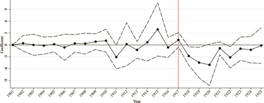
Economic growth and flu mortality: flexible specification
The coefficients are negative and statistically significant starting in 1918, when the pandemic took place, and become even more negative in 1919 and 1920, in line with our previous findings. Then, few years after the pandemic, the estimated |$ \beta _{t}$| shrink in magnitude and are not statistically different from zero after 1921. Overall, figure 4 corroborates our findings that there are no differential pre-trends in regional growth based on their exposure to the flu. Furthermore, it confirms that influenza mortality had a short-run effect on regional economic growth. We now turn to further investigate these aspects.
where |$y_{it}$| is again per-capita GDP growth in region |$i$| and year |$t$|, |$\gamma _i$| is a set of regional fixed effects, |$\delta _t$| is a full set of time fixed effects, and |$\beta $| is again our main coefficient of interest. In line with our findings of the short-run effect of the pandemic on economic growth, in this specification the variable |$Post$| is a dummy variable taking value one in the 4-year window from 1918–21. In the following, we will provide additional evidence in support of this modeling choice. Finally, we also take into account the time varying effect of control variables by interacting them time fixed effects. Our set of controls include a dummy for regions located in the North and in the Center, WWI mortality, as well as differences in pre-1918 levels of human capital and economic development.12
Panel A of table 5 presents the estimated |$\beta $| coefficients of equation 2 restricting the sample to 1901–21, in line with the evidence of the transitory growth effect of flu mortality. In column 1, the coefficient of flu mortality is --4.75. To interpret the magnitude of this coefficient, consider that it measures the average reduction in yearly growth associated with flu mortality in the 4 years 1918–21. Thus the overall effect of flu mortality sums to |$-4.75 \times 4 = -19\%$|, quite similar to the sum of the estimated coefficients reported in column 4 of table 3.
Flu mortality and economic growth: difference-in-differences specification
| Panel A: baseline | ||||
|---|---|---|---|---|
| (1) | (2) | (3) | (4) | |
| Flu mortality |$\times $| post | -4.758* | -3.526** | -3.831*** | -3.491** |
| [2.272] | [1.346] | [1.042] | [1.315] | |
| Observations | 336 | 336 | 336 | 336 |
| R-squared | 0.945 | 0.975 | 0.980 | 0.985 |
| Panel B: excluding WWI years | ||||
| (1) | (2) | (3) | (4) | |
| Flu mortality |$\times $| post | -5.047* | -3.706** | -4.023*** | -3.372** |
| [2.513] | [1.436] | [1.150] | [1.414] | |
| Observations | 272 | 272 | 272 | 272 |
| R-squared | 0.943 | 0.974 | 0.979 | 0.983 |
| WWI mortality |$\times $| years FE | No | Yes | Yes | Yes |
| Literacy 1911 |$\times $| years FE | No | No | Yes | Yes |
| GDP pc 1900 |$\times $| years FE | No | No | No | Yes |
Notes: The regressions are estimated on regional panel data for 1901–1921. The dependent variable is the rate of growth of per capita GDP. The variable |$Post$| is a dummy variable taking value one after 1917. Panel A includes the 1901–1921 period. Panel B excludes the period in which Italy was involved in WWI: 1915–1918. The |$Post$| dummy takes value one after 1917 in panel A and after 1918 in panel B. All regressions include regional fixed effects, year fixed effects, and an interaction of a dummy taking value one for regions located in the Center-North interacted with year fixed effects. Control variables are interacted with the full set of year fixed effects. Robust standard errors clustered at the regional level are reported in brackets. ***indicates significance at the 1% level, **indicates significance at the 5% level, *indicates significance at the 10% level.
In column 2, we control for WWI mortality, which is constructed as a time-invariant variable as flu mortality, interacted with year fixed effects. In column 4, we take into account pre-existing differences in human capital by controlling for the 1911 literacy rate interacted with year fixed effects. In column 5, we also consider differences in pre-existing level of economic development by controlling for GDP per capita in 1900 again interacted with year dummies. Remarkably, the coefficient remains of the hypothesized sign of statistically significant. Panel B of table 5 excludes the years in which Italy took part to WWI: 1915–18. Reassuringly, the estimated coefficients are quite similar to the ones reported in Panel A, suggesting that the results are not driven by the use of the war years. Furthermore, Appendix table A.4 shows that our results are nearly identical when correcting the standard errors for spatial correlation of the error term.
To further strengthen the robustness of our analysis, we test formally for the absence of pre-trends in regional growth rates and explore further the potential long-lasting effects of the pandemic on economic growth. We do so in table 6. For comparison with previous estimates, in column 1, we report the estimated coefficient column 4, table 5, in which we set the time window to 1901–21. In column 2, we estimate the same specification but restrict the sample to 1913–1921. The estimated coefficient is negative and statistically significant. In columns from 3 to 6 we perform a placebo test: we check if flu mortality affected growth in various sub-samples before the pandemic period. The estimated coefficient is never statistically distinguishable from zero. These results strongly support the so-called parallel trend assumption of the difference-in-differences model.
Rolling estimates
| Actual cutoff | Placebo cutoffs | Persistence | |||||
|---|---|---|---|---|---|---|---|
| Post: | 1918–1921 | 1905–1908 | 1908–1911 | 1911–1914 | 1914–1917 | 1921–1924 | |
| Sample: | 1901–1921 | 1913–1921 | 1901–1908 | 1903–1911 | 1906–1914 | 1909–1917 | 1916–1924 |
| (1) | (2) | (3) | (4) | (5) | (6) | (7) | |
| Flu mortality |$\times $| post | -3.491** | -4.075* | 0.007 | -0.163 | -1.270 | 1.750 | 0.791 |
| [1.315] | [2.030] | [0.553] | [0.616] | [0.846] | [1.653] | [0.666] | |
| Observations | 336 | 144 | 128 | 144 | 144 | 144 | 144 |
| R-squared | 0.985 | 0.992 | 0.875 | 0.847 | 0.896 | 0.965 | 0.994 |
Notes: The regressions are estimated on regional panel data over the sample period indicated in column headings. The dependent variable is the rate of growth of per capita GDP. The variable |$Post$| is an indicator variable taking value one for the years indicated in column heading. Control variables are interacted with the full set of year indicators. Robust standard errors clustered at the regional level are reported in brackets. ***indicates significance at the 1% level, **indicates significance at the 5% level, *indicates significance at the 10% level.
In the last column of table 6, we explore whether the effect of flu mortality on economic growth can still be detected in the 4-year window 1921–24. In line with our previous findings, 4 years after the pandemic the estimated coefficient is not statistically different from zero (0.79 with large standard errors). This finding further supports the econometric strategy implemented in table 5 and the short-run effect of the pandemic on growth.
In figure 5, we show graphically the results by plotting the estimated coefficients and their confidence intervals for several 4-year time windows, including both placebo periods before the pandemic, as well as the pandemic years and those after. Quite clearly, influenza mortality affects growth only in 1918–21. This provides strong evidence in support of the absence of pre-treatment differential trends, and on the transitory effect of the flu on local economic growth.
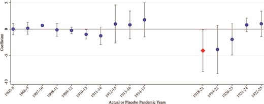
Rolling estimates
7. Heterogeneous effects and industrialization
Having explored the link between the influenza and growth, to shed further light on the potential mechanisms at work, in this section we explore the role of attenuating and aggravating factors on regional growth. We present the results in table 7.
In column 1 and 2 of table 7, we split the sample based on whether the region is above or below the median value of the 1911 literacy rate (which is 50%). The estimated coefficient is slightly larger in regions where human capital, as proxied by literacy, was initially low (column 2). This finding is in line with the historical literature suggesting that in Italy the scarcity of doctors and other medical staff enhanced the adverse effects of the flu (Tognotti 2015). Yet, this finding should be interpreted with caution, because the difference between the two coefficients is small and not statistically different from zero, possibly due to the small sample size.
In columns 3 and 4, we split the sample based on whether the region is above or below the median value of population density in 1911 (which is 110 people per |$km^2$|). The coefficient in column 3 is significantly larger (in absolute value) than the one in column 4. In columns 5 and 6, we split the sample based on whether the region is above or below the median value of the share of labor in manufacturing in 1911 (which is 20%). The estimated coefficient is significantly larger (in absolute value) in regions with high pre-pandemic share of labor in manufacturing (column 5). These findings are in line with the idea that flu mortality induced greater fear of contagion in more densely populated and more industrialized regions, where people could more likely observe how deadly the disease was.
Overall, the heterogeneous effects presented in columns from 3 to 6 indicate that the pandemic was associated with a reduction in the demand for goods and services, in turn harnessing economic growth. This hypothesis is broadly consistent with the importance of demand-side mechanisms emphasized in Basco et al. (2021) in the context of Spain.
After WWI, Italy was a predominantly rural society, with 59% of the labor force employed in agriculture, 24% in industry, and 17% in the service sector, and with less than one third of the population living in municipalities with more than 20,000 inhabitants (Malanima & Zamagni 2010, table A1). During the 1920s and 1930s, the process of industrialization was important for explaining the pattern of long-run regional development and labor force distribution (Carillo 2021). Although the country growth rate did not keep up with other advanced economies, in the interwar period, industrial output overtook agricultural output (Malanima & Zamagni 2010). It is possible that supply-side effects (such as a labor productivity slowdown) and demand-side mechanisms may have induced a reallocation of industrial production towards regions less affected by the pandemic, leading to long-lasting effects on industrial development.
To test this hypothesis, we merge data on regional employment in the manufacturing employment (see Section 4 for sources) with our mortality data. Employment data are available only for the census years (1901, 1911, 1921, 1931, and 1936), but this allows us to check whether flu mortality had any effect on manufacturing employment in 1921 (3 years after the pandemic) and subsequent years. Table 8 presents the results.
Flu mortality and economic growth: sample splits
| Literacy | Population density | Manufacturing | ||||
|---|---|---|---|---|---|---|
| High | Low | High | Low | High | Low | |
| (1) | (2) | (3) | (4) | (5) | (6) | |
| Flu mortality |$\times $| post | -3.340*** | -4.490* | -5.868*** | -1.324* | -5.713*** | -1.865 |
| [0.826] | [1.982] | [1.065] | [0.637] | [1.422] | [1.201] | |
| Observations | 168 | 147 | 168 | 168 | 168 | 168 |
| R-squared | 0.984 | 0.988 | 0.982 | 0.994 | 0.982 | 0.992 |
Notes: The table presents sample splits based on whether the variables indicated in column headings, which are all measured in 1911, are above or below the median. The regressions are estimated on regional panel data for 1901–1921. The dependent variable is the rate of growth of per capita GDP. The variable |$Post$| is an indicator variable taking value one after 1917. Control variables include a dummy taking value one for regions located in the Center-North, WWI mortality rate, and 1911 literacy rate, each interacted with the full set of year indicators. Robust standard errors clustered at the regional level are reported in brackets. ***indicates significance at the 1% level, **indicates significance at the 5% level, *indicates significance at the 10% level.
Flu mortality and industrialization
| (1) | (2) | (3) | (4) | |
| Flu mortality | -1.670** | -1.837** | -2.153* | -3.495*** |
| [0.588] | [0.682] | [1.102] | [1.011] | |
| Flu mortality—1 period lag | -0.668 | -0.984 | -3.494* | |
| [0.895] | [1.529] | [1.803] | ||
| Flu mortality—2 periods lag | -0.949 | -4.120 | ||
| [1.949] | [2.462] | |||
| WWI mortality | 0.382 | 0.673 | 1.269 | 0.041 |
| [0.419] | [0.483] | [0.843] | [1.145] | |
| WWI mortality—1 period lag | 1.161 | 1.758 | -0.540 | |
| [0.846] | [1.373] | [1.864] | ||
| WWI mortality—2 periods lag | 1.790 | -1.113 | ||
| [1.607] | [2.385] | |||
| Observations | 80 | 80 | 80 | 80 |
| R-squared | 0.091 | 0.116 | 0.177 | 0.291 |
| Region FE | Yes | Yes | Yes | Yes |
| Time trend | No | No | No | Yes |
Notes: The regressions are estimated on regional panel data in 1901–1936. The dependent variable is the year/region share of labor force employed in manufacturing. Robust standard errors clustered at the regional level are reported in brackets. ***indicates significance at the 1% level, **indicates significance at the 5% level, *indicates significance at the 10% level.
Since there was no census conducted in 1918, table 8 column 1 assigns flu mortality to 1921, the closest year to the year of the pandemic.13 We interpret the coefficient as the short- run effect of flu mortality on manufacturing employment. As before, we control also for WWI mortality. All regressions include regional level fixed effects. The estimated coefficient of flu mortality is negative (-1.67) and statistically different from zero at the 5% level but small in terms of economic significance. For instance, comparing regions with 1% flu mortality with regions with 1.5% mortality is associated to a reduction in the share of manufacturing employment of 0.8%. The estimated coefficient of WWI mortality is not statistically different from zero.
In table 8 column 2 we explore whether the effect of flu mortality persisted throughout the 1920s, introducing the lagged value of flu mortality in the regression. The coefficient is negative but not statistically different from zero. In column 3 we add a second lag and again the coefficient is negative but not statistically significant. In column 4, we check the robustness of the results adding a linear and quadratic trend. Interestingly, the estimated coefficients are negative and significant only for 1921 (at the 1% level) and 1931 (at the 10% level) but are insignificant for 1936. This finding confirms that 1918 flu mortality did not have long-lasting effects on industrialization and economic growth, in line with our previous findings.
8. Conclusions
In this paper, we conducted an empirical investigation of the link between pandemics and local economic growth in the context of the Italian 1918 influenza. Since public non-pharmaceutical interventions were either limited or mostly ineffective, the pandemic caused about 600,00 deaths in a population of 36 million but distributed differently across regions. This variability allowed us to estimate the effect of flu mortality on regional per capita GDP growth.
The paper finds a strong and significant adverse effect of the pandemic on regional growth. In particular, comparing regions with the lowest and highest mortality rates there was negative GDP per capital growth of around 6.5%. The sign and magnitude of our estimated coefficients are comparable with recent findings for the cross country effect of the 1918 influenza pandemic on economic growth (Barro et al. 2020). This result is robust to the effect of different initial conditions, differential regional growth trends before the pandemic, and potential interactions of initial conditions with flu mortality rates. We also find that the effect of the pandemic was stronger in more densely populated regions and in regions with higher share of manufacturing employment.
Our regressions show a short-run effect of flu mortality on regional economic growth, in line with recent studies of the 1918 pandemic across localities in other countries. Our findings do not rule out that the 1918 influenza had long-term effect on the level of economic development, which has been documented in other works studying the long-lasting economic consequences of diseases. A thorough analysis of the long-term consequences of the flu pandemic in Italy would require additional data and an empirical strategy able to control for the political and economic development that took place in Italy in the late 1920s. Thus, it is left for future research.
The limited interventions implemented to contain the pandemic combined with the inadequate health infrastructure that characterized many parts of Italy after WWI make the Italian historical experience of the Great Influenza an important case to cast light on the economic consequences of pandemics in developing countries where it is impossible to implement lockdown policies or where health care systems are incapable of protecting citizens. The Italian case could be useful to compare the recessionary effects of pandemics in the absence of interventions with the potentially harmful effects of interventions aimed at containing it. Given that exposure to pandemics depends also on pre-existing living standards, our findings should be interpreted cautiously and possibly considered an upper bound of the effects of pandemics on local economic growth. We hope that this study will stimulate future exploration of this important link and shed light on the heterogeneous effects of pandemics across localities and individuals.
Acknowledgments
We thank Paolo Malanima and Luigi Pistaferri for very helpful discussion and insights, Andrea Graziosi, Luigi Guiso, Franco Peracchi, and seminar participants at Bocconi, CSEF, the Società Italiana degli Economisti (SIE), and Parthenope University for comments, and Ministero dell'Istruzione, dell'Università e della Ricerca (MIUR) for financial support (PRIN Grant No. 2017RHFXK4).
Footnotes
Daily deaths peaked on October 7 in Naples (256 cases), October 16 in Milan (127), October 18–19 in Turin (119 deaths), and October 19 in Rome (226 deaths).
There are also reports showing that even at end September and early October 1918 when the epidemics was near its peak, large gatherings continued for religious or political reasons.
For a review of the economic history of Italy over the period of study and beyond see Malanima & Zamagni (2010), among others.
Studies on the consequences of the 1918 influenza include also long-run effects on human capital and other childhood outcomes (Almond 2006; Guimbeau et al. 2020; Havari & Peracchi 2017; Percoco 2016), and social trust (Le Moglie et al. 2020), among others.
Not all economic historians agree with the fact that the 1918 flu epidemic had a large impact on the economy. According to Barry Eichengreen (interviewed by John Cassidy for the New Yorker on March 18, 2020), the economic impact of the 1918 pandemic in the USA was relatively mild: “The flu had a big negative impact on retail sales, but, according to the available statistics, the overall economy didn’t fall into a recession. There was eventually a slump, in 1920–21, but Eichengreen and other economic historians have typically attributed it to the Federal Reserve raising interest rates to head off inflation”.
They also estimate the effect of death rates on consumption and asset prices. The effect on the consumption growth rate has the same sign as GDP and is somewhat larger in magnitude. The effect of the flu death rate on both realized real returns on equity and short-term government bills is negative but only statistically different from zero for government bills.
See Weil (2014) for an overview of the literature on health and economic growth.
Unfortunately, for the study period, yearly GDP data at finer levels of aggregation (province or municipality) are unavailable. After Italian unification, administration was the responsibility of central government, provinces, and municipalities, with regions statistical units encompassing several provinces. They were introduced formally with the 1948 Constitution of the Republic but became effective only after the 1970 regional elections.
For instance, |$\beta _{1}$| is an estimate of the effect of 1918 mortality on 1919 growth, conditioning on the estimated effects on 1918 growth and on the lagged effects of mortality on 1921 and 1922 growth. Similarly, the coefficient of the 2-year lag estimates, |$\beta _{2}$|, is an estimate of the effect of 1918 mortality on 1920 growth, conditioning on its effects in 1918, 1919, and 1921, and so forth.
We introduced a dummy variable that takes the value 1 for regions specialized in heavy industries in what is known as the “industrial triangle” of Lombardy, Piedmont, and Liguria, and its interaction with flu mortality. While the estimated coefficient of the variable “industrial triangle” is not statistically different from zero, the coefficient of the interaction term is negative and significant, suggesting that the adverse effect of influenza on growth was stronger in regions characterized by high capital intensity.
Estimates are similar if we also control of pre-pandemic log of population density interacted with year dummies.
While the flexible specification with the manufacturing data is not ideal given the small sample size, results using this specification are similar to the one displayed in table 8, and available on request.
References
Appendix A. Robustness
Alternative specifications
| (1) | (2) | (3) | (4) | (5) | (6) | |
| Excluding | Excluding | |||||
| Campania | Veneto | |||||
| Flu mortality | -0.104 | -0.126 | -0.519 | -1.935* | -1.826** | -1.826 |
| [0.719] | [0.879] | [0.771] | [0.921] | [0.803] | [1.909] | |
| Flu mortality—1 year lag | -13.390*** | -13.949*** | -14.246*** | -16.244*** | -16.080*** | -16.080*** |
| [2.113] | [2.574] | [2.287] | [3.447] | [3.537] | [3.284] | |
| Flu mortality—2 years lag | -4.756* | -4.722 | -5.649** | -3.925 | -3.813 | -3.813* |
| [2.293] | [2.868] | [2.406] | [2.254] | [2.293] | [2.095] | |
| Flu mortality—3 years lag | -3.595** | -3.988* | -4.481** | 0.453 | 0.303 | 0.303 |
| [1.496] | [1.869] | [1.589] | [0.485] | [0.472] | [1.539] | |
| Flu mortality—4 years lag | -0.172 | -0.182 | -0.748 | 5.239*** | 4.566*** | 4.566** |
| [1.123] | [1.431] | [1.172] | [0.862] | [0.915] | [2.062] | |
| Observations | 464 | 435 | 435 | 464 | 464 | 464 |
| R-squared | 0.726 | 0.720 | 0.727 | 0.822 | 0.825 | 0.827 |
| WWI death rate | Yes | Yes | Yes | Yes | Yes | Yes |
| Time trend | Yes | Yes | Yes | Yes | Yes | Yes |
| Region FE | Yes | Yes | Yes | Yes | Yes | Yes |
| National GDPpc | No | No | No | Yes | Yes | Yes |
| War years FE | No | No | No | No | Yes | Yes |
| Two-way clustering SE | No | No | No | No | No | Yes |
Notes: The regressions are estimated on regional panel data for 1901–1929. The dependent variable is the rate of growth of per capita GDP. For comparison, column 1 reproduces the same regression of the last column of Table 4. Columns 2 and 3 exclude, respectively, regions with the highest and lowest mortality rates (Campania and Veneto). WWI The “WWI Death rate” variables include the current value and four lags of the WWI death rate. The “Time trend” variables include a linear and quadratic time trend. National GDP per capita includes linear, quadratic, and cubic terms of real national GDP per capita. War Years fixed effect is a dummy taking value one in the years in which Italy was in war (from 1915 to 1918). Robust standard errors clustered at the regional level are reported in brackets, except column 6 where standard errors are adjusted for two-way clustering over regions and years. ***indicates significance at the 1% level, **indicates significance at the 5% level, *indicates significance at the 10% level.
Controlling for age structure and sex ratio
| (1) | (2) | (3) | (4) | |
| Flu mortality | -0.230 | -0.205 | -0.295 | -0.302 |
| [0.555] | [0.567] | [0.588] | [0.601] | |
| Flu mortality—1 year lag | -13.619*** | -13.574*** | -13.738*** | -13.749*** |
| [1.805] | [1.837] | [1.870] | [1.899] | |
| Flu mortality—2 years lag | -4.985** | -4.939** | -5.104** | -5.115** |
| [2.014] | [2.021] | [2.073] | [2.073] | |
| Flu mortality—3 years lag | -3.824*** | -3.779*** | -3.944*** | -3.955*** |
| [1.179] | [1.217] | [1.248] | [1.285] | |
| Flu mortality—4 years lag | -0.298 | -0.273 | -0.364 | -0.371 |
| [0.965] | [0.969] | [0.996] | [0.998] | |
| Observations | 464 | 464 | 464 | 464 |
| R-squared | 0.726 | 0.726 | 0.726 | 0.727 |
| WWI death rate | Yes | Yes | Yes | Yes |
| Initial GDP pc | Yes | Yes | Yes | Yes |
| Time trend | Yes | Yes | Yes | Yes |
| Share of age |$\in [20;40] $| | No | Yes | No | Yes |
| Sex ratio | No | No | Yes | Yes |
Notes: The regressions are estimated on regional panel data for 1901–1929. The dependent variable is the rate of growth of per capita GDP The table shows that the coefficient of flu mortality does not change appreciably when we introduce the age structure and the gender ratio as additional controls. For comparison, column 1 reproduces the same regression of column 4 of Table 4. Column 2 adds the regional share of the population aged 20 to 40 in 1911. Column 3 adds the regional sex ratio (number of males over number of females) in 1911. Robust standard errors clustered at the regional level are reported in brackets. ***indicates significance at the 1% level, **indicates significance at the 5% level, *indicates significance at the 10% level.
Robustness to including flu mortality in 1919
| (1) | (2) | (3) | (4) | (5) | |
| Flu mortality (1918–19) | 0.481*** | -0.307 | -0.401 | -0.341 | -0.274 |
| [0.124] | [0.428] | [0.472] | [0.493] | [0.634] | |
| Flu mortality (1918–19)—1 year lag | -12.598*** | -11.151*** | -11.323*** | -11.365*** | -11.243*** |
| [0.702] | [1.431] | [1.516] | [1.548] | [1.809] | |
| Flu mortality (1918–19)—2 year lag | -6.866*** | -4.201** | -4.374** | -4.334** | -4.212** |
| [0.737] | [1.576] | [1.681] | [1.713] | [1.954] | |
| Flu mortality (1918–19)—3 year lag | -2.877*** | -3.353*** | -3.526*** | -3.398*** | -3.275** |
| [0.171] | [0.966] | [1.036] | [1.047] | [1.319] | |
| Flu mortality (1918–19)—4 year lag | 1.082*** | -0.464 | -0.558 | -0.386 | -0.319 |
| [0.194] | [0.790] | [0.839] | [0.815] | [0.951] | |
| Observations | 464 | 464 | 464 | 464 | 464 |
| R-squared | 0.564 | 0.716 | 0.718 | 0.727 | 0.728 |
| WWI death rate | No | Yes | Yes | Yes | Yes |
| Initial GDP pc | No | No | Yes | Yes | Yes |
| Time trend | No | No | No | Yes | Yes |
| Region FE | No | No | No | No | Yes |
Notes: The regressions are estimated on regional panel data for 1901–1929. The dependent variable is the rate of growth of per capita GDP Robust standard errors clustered at the regional level are reported in brackets. ***indicates significance at the 1% level, **indicates significance at the 5% level, *indicates significance at the 10% level.
Robustness to spatial correlation adjustment: difference-in-differences specification
| Panel A: baseline | ||||
|---|---|---|---|---|
| (1) | (2) | (3) | (4) | |
| Flu mortality |$\times $| post | -4.758** | -3.526** | -3.831*** | -3.491*** |
| [2.279] | [1.480] | [1.418] | [0.983] | |
| Observations | 336 | 336 | 336 | 336 |
| R-squared | 0.055 | 0.064 | 0.092 | 0.045 |
| Panel B: excluding WWI years | ||||
| (1) | (2) | (3) | (4) | |
| Flu mortality |$\times $| post | -5.047** | -3.706** | -4.023*** | -3.372*** |
| [2.383] | [1.538] | [1.513] | [1.045] | |
| Observations | 272 | 272 | 272 | 272 |
| R-squared | 0.066 | 0.076 | 0.106 | 0.041 |
| WWI mortality |$\times $| years FE | No | Yes | Yes | Yes |
| Literacy 1911 |$\times $| years FE | No | No | Yes | Yes |
| GDP pc 1900 |$\times $| years FE | No | No | No | Yes |
Notes: The regressions are estimated on a regional panel data for 1901–1921. The dependent variable is the rate of growth of per capita GDP. The variable |$Post$| is a dummy variable taking value one after 1917. All regressions include regional fixed effects, year fixed effects, and an interaction of a dummy taking value one for regions located in the Center-North interacted with year fixed effects. Control variables are interacted with the full set of year fixed effects. Panel A includes the 1901–1921 period. Panel B excludes the period in which Italy was involved in WWI: 1915–1918. The standard errors reported in brackets are adjusted for spatial correlation using the procedure by Conley (1999) and the software by Colella et al. (2019). The adjustment takes into account any arbitrary correlation of the error term within a 1000-kilometers radius from the regional capitals, and within a 20-years time lag. ***indicates significance at the 1% level, **indicates significance at the 5% level, *indicates significance at the 10% level.
Appendix B. Data description and sources
Summary statistics
| Variable | Mean | Std. Dev. | Min. | Max. | N |
|---|---|---|---|---|---|
| Growth GDP per capita 1901–29 | 0.010 | 0.058 | -0.253 | 0.168 | 464 |
| Labor share in manufacturing 1901–36 | 0.212 | 0.067 | 0.106 | 0.422 | 80 |
| Flu mortality rate 1918 | 0.013 | 0.003 | 0.007 | 0.019 | 16 |
| WWI mortality rate 1915–18 | 0.015 | 0.003 | 0.009 | 0.021 | 16 |
Gross domestic product per capita: To explore the short-term link between flu mortality and economic activity, our study requires yearly GDP data. For this purpose, we rely on the series published by Daniele & Malanima (2011) for the 16 Italian regions. We are aware of the existence of other historical regional GDP data (Felice, 2013), and on the debate around them (Daniele & Malanima, 2014b), but to the best of our knowledge other sources provide regional GDP data only by decade, and thus cannot be used to estimate the short-term effects of the pandemic.
Flu mortality rate: The variable is defined as the number of deaths in 1918 for influenza and pneumonia (specifically we sum influenza, broncopolmonite, and polmonite) over population in 1911. The data are displayed in Table B.2. The source for flu mortality is the Mortality Statistics Volume for 1918 (Statistica delle Cause di Morte 1918) published by the Ministry of the National Economy. The source for population is the Italian Statistical Office Population Census.
There is no perfect way to measure flu mortality. One approach is to use official records. However, number of deaths for influenza and pneumonia may underestimate the actual number of deaths because official records may not count people that died from other diseases because of influenza contagion. On the other hand, the official numbers may over-estimate true mortality because they attribute to the pandemic mortality for influenza and pneumonia that would have occurred in the absence of the pandemic. An alternative approach is to estimate statistically excess mortality with respect to normal times.
We follow the first approach because we want to avoid ad-hoc decisions. But we also compare our estimate of flu mortality with existing estimates based on other approaches. We estimate 453,501 deaths in 1918 and 108,384 in 1919, a total of 561,885 deaths for influenza and pneumonia. An early study by Mortara (1925) found that deaths from August 1918 to March 1919 exceeded mortality for the same months of 1911–1913 by 532,457 units. Adding deaths of soldiers recorded by military authorities he raised the number to 600,000. Fornasin et al. (2018) use official death statistics and the Albo d’oro, a roll of honor of the Italians fallen in the WWI, placing the estimate at 466,000. Ansart et al. (2009) use an excess mortality approach. Using monthly data for the whole country they estimate a death toll of 544,288 individuals. These numbers are actually not far from our estimate of 532,457 deaths.
Furthermore, given that we control for WWI deaths, our estimated coefficients are potentially unaffected by military deaths due to influenza during the war. Finally, given that we rely on variability across regions, measurement error in flu mortality would inflate standards errors without affecting the estimated coefficient under the assumption that measurement error is uncorrelated with regional economic growth in the year of the pandemic. Nevertheless, even if measurement error in influenza mortality was greater in regions characterized by slow growth, it would induce a bias that is opposite in sign to the coefficient of interest.
Flu mortality and WWI mortality by region
| Region | Flu mortality in 1918 | Flu mortality in 1919 | WWI mortality | Population (000) in 1911 |
| Abruzzi | 20165 | 3939 | 22121 | 1512 |
| Apulia | 36639 | 6208 | 28173 | 2195 |
| Basilicata | 7505 | 1903 | 7316 | 486 |
| Calabria | 21963 | 4866 | 19965 | 1526 |
| Campania | 57789 | 13766 | 42315 | 3102 |
| Emilia | 31587 | 8498 | 49391 | 2813 |
| Latium | 24791 | 4083 | 16012 | 1771 |
| Liguria | 14924 | 4963 | 12440 | 1207 |
| Lombardy | 58780 | 13868 | 79437 | 4889 |
| Marche | 12410 | 3073 | 19395 | 1145 |
| Piedmont | 39078 | 12407 | 49982 | 3495 |
| Sardinia | 14147 | 3556 | 13600 | 868 |
| Sicily | 46111 | 8855 | 44197 | 3812 |
| Tuscany | 33009 | 7743 | 46860 | 2670 |
| Umbria | 7904 | 2129 | 12860 | 614 |
| Veneto | 26699 | 8527 | 63124 | 3737 |
| Total | 453501 | 108384 | 527188 | 35842 |
Notes: Column 2 reports the number of deaths in 1918 for influenza and pneumonia. Column 3 reports the number of deaths in 1919 for influenza and pneumonia. Column 4 reports the number of military deaths in WWI. Column 5 reports the population in 1911 (in thousands). See Appendix B for data sources.
World War I death rate: The variable is defined as the total number of military deaths during WWI over population in 1911. The year of death is not always certain and often military deaths occur with significant lags. Thus, our variable for WWI death rates takes value zero for the years before 1915 (the year in which Italy joined the war) and after 1918. Over the war years the variable equals the total number of military deaths due to WWI over population as of 1911. Source: Albo d’Oro archive of the Institute for History and Resistance and Contemporary Society (Istoreco).
Manufacturing Labor Force: Share of labor force employed in manufacturing in 1901, 1911, 1921, 1931, and 1936 (Daniele & Malanima, 2014a, Tab. 1).
Human Capital: We use the literacy rate in 1911 (Felice, 2007, Tab.6) and the Human Development Index (Felice, 2007, Tab.9;10) for the year 1911.
