


Abstract
We measure the impact of a reduction in transaction costs on crop area and production of smallholder tobacco growers in Malawi. For identification, we exploit the introduction of an additional tobacco auction floor. Estimations are based on annual data by extension planning area. A 10 per cent reduction in distance to auction floor is shown to increase crop area and production around 4 and 10 per cent, respectively. Supply response weakens beyond a distance to auction floor of 60 km and runs along the intensive margin: existing tobacco growers improve productivity of cultivation. Impacts are robust for non-random placement of auction floors and several other threats. The results point to potentially large welfare benefits for smallholders if marketing infrastructure is improved and if more auction floors are introduced.
1. Introduction
Smallholders in developing countries can choose to produce food crops for home consumption or cash crops for the market1. High production costs, high transaction costs and high risks due to volatility of output and input prices often make subsistence farming – food production for home consumption – the optimal choice (De Janvry, Fafchamps and Sadoulet, 1991; Jayne, 1994; Fafchamps, 1999; Key, Sadoulet and De Janvry, 2000; De Janvry and Sadoulet, 2006)2. Widespread subsistence farming leads to low productivity and low growth in agriculture (see, for example, World Development Report, 2008). For several reasons, a stagnant agricultural sector is likely to obstruct economic growth of these countries: developing countries have large agricultural sectors with a comparative advantage vis-à-vis non-agricultural sectors; some authors claim that there are potentially large multiplier effects from agriculture to the remaining sectors of the economy and much less the other way around. As a consequence, few alternative growth strategies are available in developing countries other than promoting agriculture (De Janvry and Sadoulet, 2010)3.
The question arises, how can countries overcome this subsistence farming trap?4 A possible way out of this trap is to reduce transaction costs for smallholders. Transaction costs – all costs incurred in order to sell on the market – include costs of information, collection, loading and transport of goods, bargaining on prices and conditions, and monitoring and insurance, with transport costs usually considered to be the largest component. There is a broad consensus that transaction costs, which are only partly observed, are large and the key cause of not selling on the market (De Janvry and Sadoulet, 2006). Consequently, improved access to markets – not only the introduction of physical markets, but also better institutions and improved logistical and marketing infrastructure – decreases transactions costs and should, thereby, trigger smallholders to cultivate crops for the market. Transaction costs, hence, play an important role in explaining the cash crop – food crop decision.
In the current paper, we investigate how a change in marketing infrastructure, leading to reduced transport costs and improved market access, affects crop area and production of smallholder cash crop growers. The empirical work is based on tobacco marketing in Malawi: we exploit the introduction of a new tobacco auction floor in Malawi as a quasi-experiment5. This identification strategy allows us to quantify the causal impact of market access on supply. The case study focuses on smallholders that grow a cash crop for export: it is by historical coincidence and unlike most developing countries that smallholders in Malawi – and nearly exclusively smallholders, the poorest part of the population – are involved in cash crop cultivation for export. Market access is a pre-requisite for commercial farming and export-led growth could be an effective strategy for poverty alleviation and country-wide economic growth: our results show how both can be achieved.
The paper is organised as follows. In Section 1, we position this study in the literature and highlight its contribution. In Section 2, we describe the Malawi tobacco industry. In Section 3, we discuss the theoretical framework, the data and the empirical strategy. In Section 4, we present and discuss estimation results. In Section 5, we consider alternative explanations and potential threats. Section 6 summarises the findings.
2. Review of the literature
What causes farmers to grow low-yielding food crops for home consumption rather than high-return cash crops for the market? And what explains that large groups of farmers prefer not to participate in the market? Various researchers have modelled the decision to grow either subsistence crops or cash crops, and the decision to participate in the market (De Janvry, Fafchamps and Sadoulet, 1991; Goetz, 1992; Jayne, 1994; Omamo, 1998; Key, Sadoulet and De Janvry, 2000; Renkow, Hallstrom and Karanja, 2004; De Janvry and Sadoulet, 2006). Due to transactions costs, households have a tendency to get trapped into self-sufficiency and limited participation in the market explains a sluggish supply response (De Janvry, Fafchamps and Sadoulet, 1991). The wedge between producer prices for home-produced maize and consumer prices for maize purchased in the market drives the decision to cultivate food crops rather than cash crops, and this wedge is especially large in rural areas, requiring a large decrease of consumption prices to make cash crop production attractive (Jayne, 1994). Transport costs between farms and markets alone are sufficient to account for observed food-dominated cropping patterns as optimal responses (Omamo, 1998). The mutual dependence between food crop and cash crop cultivation corresponds with decisions in non-separable household models with incomplete markets (De Janvry and Sadoulet, 2006). In a generalisation of the model proposed by Goetz (1992), Key, Sadoulet and De Janvry (2000) show that both proportional and fixed transaction costs matter: supply response to a price increase is partly due to producers who enter the market (60 per cent), and partly due to those producers who are already sellers on the market (40 per cent). Several researchers investigated the implications of high transaction costs empirically (e.g. Minten and Kyle, 1999, Fafchamps and Vargas Hill, 2005, Jacoby and Minten, 2009). In choosing between selling to an itinerant trader at the farm gate and carrying output to the nearest market town, farm households are more likely to sell to the market when the quantity sold is large and the market is close by, and wealthy farmers are more likely to travel to distant markets (Fafchamps and Vargas Hill, 2005). Differences in food prices between producer regions and urban areas are explained by transportation costs, and road quality is the key determinant of transportation costs (Minten and Kyle, 1999). Large gains in income may be realised from improved road infrastructure for remote households, but are modest relative to improved non-farm earning opportunities in town (Jacoby and Minten, 2009). Another strand of empirical work focuses on the impact of search costs – a component of transaction costs – on behaviour and market prices. Improved market information for households is shown to significantly raise the probability of participating in the market as a seller or a buyer (Goetz, 1992). Various studies have exploited the roll-out of mobile phones to investigate impact on market prices and behaviour (Jensen, 2007; Muto and Yamano, 2009; Aker, 2010). Using IV and matching techniques, Negri and Porto (2016) show that membership of burley tobacco clubs in Malawi causes a significant increase in output per acre (40–74 per cent) and in sales per acre (45–89 per cent), highlighting an important channel that affects output and productivity in Malawi tobacco production. In a particularly relevant study on the soy market in the central Indian state of Madhya Pradesh, Goyal (2010) investigates the impact of a direct marketing channel for farmers, in the form of internet kiosks offering price information and warehouses offering quality testing and direct sales to the end-user (a private company), thereby bypassing intermediary traders. As a result, monthly soybean prices increased (1.7 per cent), price dispersion decreased (less than −1 per cent) and area under soy cultivation increased (+19 per cent).
The literature offers persuasive evidence, both theoretical and empirical, for the key role that transaction costs play in explaining supply response and subsistence farming. In the current paper, we complement the work on the choice between food and cash crops by showing empirically the importance of transport costs in supply response of cash crop growers. Similar to Goyal (2010), we investigate the impact of a change in marketing infrastructure. In particular, we study tobacco producers in Malawi, and how improved market access – caused by the introduction of a new auction floor – affects crop area and production of smallholders. Tobacco in Malawi is by far the most important cash crop, grown in nearly all Malawi districts and, by regulation, exclusively sold on auction floors. Transaction costs, costs associated with selling tobacco through auctions – estimated to be 14.5–22.5 per cent of sales value (FAO, 2003)–are fully on account of tobacco growers. In 2004, an additional auction floor started operations in Chinkhoma, Kasungu district, on top of the three already operational auction floors (in Limbe, Kanengo and Mzuzu). The new auction floor offered farmers in its neighbourhood an opportunity to produce tobacco in a commercially viable way. For the empirical estimations, we make use of annual smallholder production and area data at Extension Planning Area (EPA) level, in total 198 EPAs, covering the whole of Malawi, from crop seasons 2003/2004 to 2009/2010, a period of seven years. We find a statistically significant impact of transport costs on production and crop area. A 10 per cent reduction in distance to auction floor is shown to increase crop area and production by around 4 and 10 per cent, respectively. A reduction of transport costs is, thereby, shown to trigger commercial agriculture and confirms results of other empirical work on the role of transport costs (Key, Sadoulet and De Janvry, 2000; Renkow, Hallstrom and Karanja, 2004; Jensen, 2007). Additionally, we contribute to the literature that seeks to reveal constraints to export growth strategies and to highlight the potential of export-led growth strategies in poverty alleviation (Balat, Brambilla and Porto, 2009). Employing a wider perspective, our results complement recent economic geography-based literature, using geo-referencing to estimate the impacts of road or rail networks on economic activity and urbanisation in sub-Sahara Africa (see, for example Jedwab and Moradi, 2016; Storygard, 2016). A final remark on the reputation of tobacco as a cash crop: we are aware of the negative status of tobacco, especially since the 2003 WHO Framework Convention of Tobacco Control6. However, in the current research tobacco is only instrumental to measure supply response, to find ways to promote commercial agriculture, to increase welfare of poor farmers and to enhance economic development.
3. The Malawi tobacco industry7
3.1. The role of tobacco in the domestic economy of Malawi
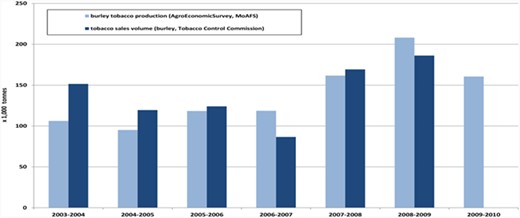
Tobacco is, by far, the most important export product of Malawi accounting for a share of 45–65 per cent of total merchandise exports (1994–2009, National Statistical Office [NSO] data). The second largest single export product (either tea or sugar) accounts for only a small fraction of total merchandise exports. Tobacco exports also account for about 60 per cent of foreign exchange earnings. Virtually, all tobacco is exported: Malawi does not have a domestic cigarette industry. The direct contribution of tobacco to Gross Domestic Product (GDP), measured as the export value of tobacco in terms of GDP, varies from 9 to 16 per cent (1994–2009, National Statistical Office). Tobacco is cultivated by 19 per cent of the smallholder sector, around 375,000 households (2004). The bulk of the tobacco growing households – around 65 per cent – are poor or very poor. In the period from 2003 to 2010, aggregate smallholder crop area allocated to tobacco ranged from 141,000 to 184,000 hectares, and smallholder crop production varied from 95 to 208 thousand tons (source: Agro Economic Survey [AES], Ministry of Agriculture and Food Security [MoAFS]). Using a methodology employed by the FAO (FAO, 2003), we estimate direct employment in tobacco production and marketing (including processing, transport, auctioning and research) to vary from 11 to 19 per cent of total labour supply during 2000–2009. Tobacco exports also generate a major contribution to government tax revenue. Tobacco taxes and levies add up to an estimated share of total government tax revenue of 30 per cent in 2000 and around 20 per cent in 2008 (FAO, 2003; Jaffee, 2003). The large share of tobacco proceeds that flows to the Government of Malawi makes the government a major stakeholder in the tobacco industry, potentially creating rents associated with a lack of competition, a lack of transparency and a lack of accountability (Koester et al., 2004). The role of tobacco may extend well beyond these figures, due to indirect effects, backward and forward linkages and dynamics. Some authors claim Malawi’s exports of tobacco to be the major driver of economic growth (Lea and Hammer, 2009).
3.2. Tobacco cultivation in Malawi: from colonial heritage to smallholder domination
The Special Crop Act of 1964 (the year of independence) had created a dual tobacco sector, with special privileges for estates and with restrictions for smallholders. Urged by donors to implement liberalisations in the tobacco industry, the 1993 newly elected government introduced amendments to this 1964 Special Crop Act that allowed smallholders to grow burley tobacco (Jaffee, 2003)8. The 1964 Special Crop Act was fully repealed in 1996, which included the abolishment of special marketing rights to estates. By 1996/97, all restrictions for smallholders to grow and market tobacco were removed (Diagne and Zeller, 2001). In the course of the 1990s, the change in regulation has given rise to a complete transformation from estate based to smallholder-based tobacco cultivation. From 1994 to 2002, the share of estates in tobacco production decreased from 80 per cent to less than 30 per cent (source: Tobacco Control Commission [TCC]). The change is also reflected in the shift from western-type tobacco’s (typically grown by estates) to burley tobacco (typically grown by smallholders, see also Figure 1)9. High profitability of tobacco cultivation (Place and Otsuka, 2001; Koester et al., 2004; Harashima, 2008 and Prowse and Moyer-Lee, 2014)–the only really remunerative cash crop available to smallholders – and the widespread technical knowledge on tobacco cultivation – since many farmers worked previously on estates as labourers – triggered high growth of smallholder tobacco production.
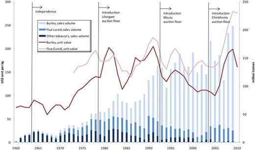
Auction sales volume and unit values of Burley and other tobacco.
Note: nominal unit values in US$ cent per kg are on the left axis and sales volume in million ton on the right axis. Unit values are sales value (in US$) divided by sales volume (in kg). `Other tobacco's' are NDDF, SDDF (Northern and Southern Division Dark Fired, respectively, so-called western type tobaccos) and Sun Air; source: TCC, Malawi.
Figure 1 also illustrates the development of burley and flue-cured auction unit values, roughly parallel, with the latter in most years higher. Visual inspection of the figure suggests that (lagged) prices move jointly with production in a more or less systematic way, reflecting a positive response of production to auction prices (also Jaffee, 2003 and our own estimates).
3.3. Tobacco marketing: farmers’ clubs, regulations, transport services and auction floors
A natural starting point to describe the tobacco auction system in Malawi are the 1990s, the period when the tobacco sector was liberalised. Transport of tobacco to auctions was – both pre- and post-liberalisation – on account of tobacco farmers. With free access to auction floors for smallholders in the 1990s, a logistical infrastructure for tobacco transport and marketing from rural areas to auction floors was emerging to service smallholder farmers. This infrastructure effectively covered the whole chain from cultivation (advise, extension, inputs and credit), to processing for trade (curing, grading, packaging, storage), transport (bundling) and marketing (licensing, selling at auction). Operations in this chain are supported and implemented by several (types of) organisations (farmers’ clubs, Malawi Rural Finance Company, intermediate buyers, the Tobacco Association of Malawi, the National Association of Smallholders Farmers of Malawi and auction floors), managed by a variety of institutions (TCC; the Auction Holdings Limited (AHL)) and regulated by continuously changing arrangements (see for details: Orr, 2000; Diagne and Zeller, 2001; Jaffee, 2003; FAO, 2003; Koester et al., 2004; Prowse and Moyer-Lee, 2014; Negri and Porto, 2016). A few observations are key to our empirical work. Most smallholders tobacco growers (more than 80 per cent) sell their tobacco directly on auction floors (Diagne and Zeller, 2001; Integrated Household Survey 2 [IHS-2] (2004/2005)). Also, transaction costs of tobacco, including transport costs, are fully on account of smallholders. Consequently, net tobacco revenues received by (most) smallholder tobacco growers increase if transaction costs decrease.
As early as 1939 tobacco was auctioned only at the Limbe auction floor, near Blantyre in the south of Malawi. In more recent years, the centre of tobacco production moved in the northern direction: auction floors were established in 1979 in Kanengo, near Lilongwe in Central Malawi; in 1993 in Mzuzu in Northern Malawi; and in 2004 in Chinkhoma in the central district Kasungu, between Lilongwe and Mzuzu (see Figure 2). Operations on all tobacco auction floors are run by a single private sector company, the AHL. The establishment of a (new) auction floor requires complementary investments from leaf merchants to properly organise after-sales processing, storage and international transport: this makes the auction floor location decision partly dependent on the investments of leaf merchants10.
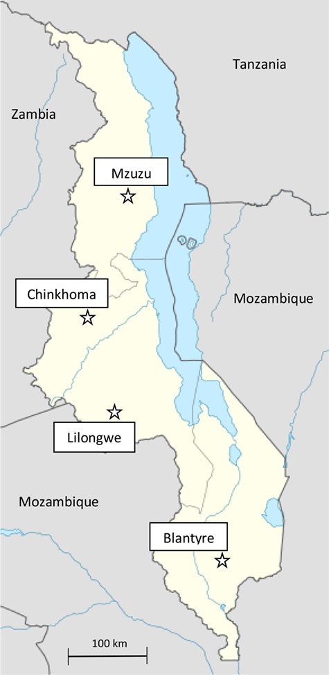
Tobacco auction floors in Malawi.
Note: the stars in the figure indicate the location of the tobacco auction floors.
Source: author.
Auction floors normally open from mid-March and close towards the end of October11. The trading process is open-outcry, with multiple buyers and one seller, while the sale of tobacco is concluded to the highest bidder. Direct trade and contract trade is only important for specialty tobacco’s (Flue Cured, NDDF and SDDF) and plays a minor role in the marketing of burley tobacco12. Note, however, that even contracted trade has to pass through the auction floors. Moreover, under the contract system, farmers still have the option to sell on the auction floor. The traditional auction system has four national sales daily: two in Lilongwe and one each in Limbe and Mzuzu. The Chinkhoma floor trades twice a week on which days Lilongwe only has one auction sale.
4. Conceptual framework, data and data sources, and empirical strategy
4.1. How do transaction costs influence farmers’ behaviour?
A reduction in transaction costs, either fixed or variable, increases the net market price of the cash crop and, thereby, shifts the balance towards increased cash crop production.
4.2. Data for analysis
The estimations in the empirical section are based on annual data of agricultural production and crop area at the level of EPAs, sourced from the Agro Economic Survey of the Ministry of Agriculture and Food Security (AES-MoAFS). EPAs are subdivisions of districts and have a median size of 400 km2, a population of around 60,000 (median), comprising around 19,000 households (median). Data on production and area by EPA are available for the crop years from 2003/2004 to 2009/2010 (seven crop years). The EPA data identify a total of 198 EPAs that cover the whole of Malawi13. Only a few of these EPAs, located in the southern districts Chikwawa and Nsanje, have no or negligible tobacco cultivation. EPA data offer the most complete and detailed information about smallholder area and production dynamics in tobacco, which is available for Malawi. None of the alternative data and data sources (IHS/NSO, TCC) allow insight into the dynamics of tobacco production and area, in a such a wide range of locations in Malawi, for a sequence of years covering the period during which the new auction floor was introduced.
Apart from EPA level production and area of a few additional crops (maize, groundnuts and pulses), there is, unfortunately, no further systematic information at EPA level available. In the estimations, we have therefore matched the EPA data with data from various other sources, in particular rainfall, prices, population and various distances, with, however, varying levels of geographical aggregation, variability and completeness. Crop prices are, for example, available for, respectively, 50–70 markets and in varying degrees of completeness. Rainfall data are available for around 30 weather stations (luckily, without missing observations). Summary statistics of the EPA level data are presented in Table A1 in Appendix A.
We approximate transport costs with road distance, from EPA to the (different) auction floors and source road distance data from Google Maps14. Potential measurement error may arise because latitude – longitude coordinates for EPAs – usually the main town or village in the EPA – will not necessarily coincide with the tobacco area in the EPA. In the procedure to identify intervention locations, we use the area size of the EPA to control for this potential error.
4.3. Intervention locations
Tobacco farmers that benefit from the introduction of the new auction floor in Chinkhoma in 2004 are identified by determining the shortest distance from EPA to the auction floor. If in 2004, the Chinkhoma auction floor has become the closest auction floor, tobacco growers in those EPAs have realised a reduction of transport costs to the auction floor. Practically, this implies that all EPAs in the districts Kasungu and Nkhotakota, a large part of locations in the districts Ntchisi, Dowa and Mchinji, and a few in the district Mzimba are intervention locations. In all, this concerns 31 EPAs/locations, 15.3 per cent of all locations.
The distribution of sales by district of origin (see Appendix F) shows that the Chinkhoma auction floor also attracts tobacco outside these districts (e.g. from Lilongwe, Rumphi and Salima districts). Adhering to the rule that ‘the Chinkhoma auction floor has become the closest auction floor’ for the identification for intervention EPAs is apparently too strict. We assume that this is caused, at least partly, by inaccuracies in the measurement of distance (see Section 4.2, the ‘Data for analysis’ paragraph). Therefore, we further add EPAs to our set of intervention EPAs, for which the distance to the new Chinkhoma auction floor become the shortest distance if we correct for the potential measurement error in the location of tobacco farmers within the EPA. Potential measurement error in distance to auction floor is approximated with the root of the EPA land area15. On these grounds, we have identified another 14 additional EPAs, summing to a total of 45 intervention EPAs, out of a total of 198 EPAs (22.7 per cent) that potentially benefit from the newly established auction floor.
4.4. Empirical strategy: basic specification
Covariates (
4.5. Empirical strategy: event plots and testing for a common trend
The outcome of this estimation, plotted in Figure 3, indicates a clear impact for all outcome variables. Impacts on production start in 2005–2006 and increase gradually over time. Impacts on crop area and yield are delayed and only show up from 2006 to 2007 or 2007 to 2008 onwards. As expected, developments in impacts of all three outcome variables run approximately parallel. Moreover, the event plots indicate that before coefficients are statistically insignificant and thereby support a common trend in the observations of both intervention and non-intervention EPAs, before the start of the new auction floor. In summary, the event plots show that the common trend assumption is satisfied, give us a sense of size, timing and persistence of impacts and make us confident to proceed with estimations. Direct evidence of increases in tobacco farm gate prices (see Appendix C), although less reliable17, further confirms these conclusions.
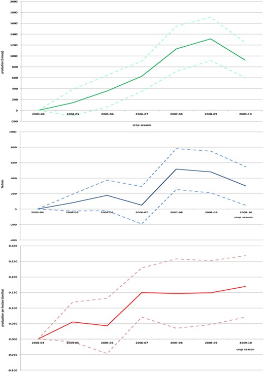
Impact of lower transport costs on production (upper), area (middle) and area productivity (lower).
Note: we estimated
4.6. Empirical strategy: using GPSs and dose – response functions
The location of the new tobacco auction floor is not randomly assigned. The auction company will have considered alternatives and investigated the optimal location for doing this investment, basing its eventual choice on an assessment of current and expected turnover of tobacco and long-run profit potential of auction services at several alternative locations. Consequently, causality may not run (only) from market access to decisions of tobacco growers to grow tobacco, but also the other way around, from (expected) tobacco production to the establishment of an auction floor. As a result, OLS estimations are potentially biased: estimates may not reflect the isolated impact of a change in transaction costs on tobacco area and production.
We propose a propensity score method to reduce the potential bias in the estimations. Unfortunately, propensity score methods are mainly developed for binary treatment variables and hence not suitable for our continuous distance to auction floor treatment variable. An extension of the propensity score method for a continuous treatment setting is developed in Hirano and Imbens, 2004, and will, hence, be used for the empirical work in this study. We briefly summarise this method and the associated STATA commands (Bia and Mattei, 2008), with particular attention to the underlying assumptions of the treatment variable and testing the balancing property. It should be noted that the applied estimation technique only reduces the potential bias generated by confounding factors, but it does not eliminate this bias. Also, and equivalent to standard propensity score matching, the extent to which bias is reduced depends on the richness and quality of control variables.
The continuous treatment corollary to binary treatment propensity scores is the generalised propensity score (GPS). Likewise, the GPS can be used to eliminate biases associated with differences in the covariates. The propensity function (r(t,x)) is defined as the density of actual treatment conditional on covariates (r(t,x) = fT|X (t,x)) and the GPS is R = (r(T,X), where T is a continuous set of treatment values. The GPS-balancing property requires that within strata with the same value of the function r(t,x), the probability of a specific value of the treatment (t) should be independent of the covariates (X). Hence, if we estimate the GPS r(t,x) within strata, it should be the same for different values of t.
The function that maps the relationship between outcome and continuous treatment is labelled the (unit-level) dose response function (Yi(t)): we are interested in the average dose response function. The dose response function is estimated at a particular level of the treatment as the average of the conditional expectation over the GPS at that particular level of the treatment, in formula: μ(t) = E [β (t; r(t;X))]. Although propensity scoring techniques are only a modest improvement over OLS, GPS and the dose response estimation that employs GPS, does offer more flexibility in functional form (see also the empirical section).
5. Estimating impact of market access on tobacco area, production and yield
Selected estimation results for our basic specification are reported in Table 1. The table reports estimations results for a basic specification, containing EPA and year-fixed effects (columns 1, 3 and 5), and a specification additionally including covariates (columns 2, 4 and 6). Unlike the event estimations from the previous section, which allowed varying responses, the specification imposes a fixed impact over the years. Following accepted practice (see Bertrand et al., 2004), we have clustered standard errors at the EPA level.
Market access in tobacco: basic specification and covariates
| Dependent variable | ln (production) | ln (area) | ln (production per hectare) | |||
|---|---|---|---|---|---|---|
| (1) | (2) | (3) | (4) | (5) | (6) | |
| ln (distance to auction floor) | −0.937*** (0.341) | −1.020*** (0.342) | −0.376* (0.226) | −0.397* (0.227) | −0.524*** (0.140) | −0.617** (0.285) |
| ln (rainfall) | 0.202* (0.116) | 0.163*** (0.058) | ||||
| ln (tobacco pricet−1) | 0.085 (0.091) | 0.055 (0.076) | 0.031 (0.048) | |||
| Trend | 0.077*** (0.028) | 0.064** (0.025) | ||||
| Number of observations | 1,152 | 1,148 | 1,152 | 1,148 | 1,152 | 1,148 |
| R2 | 0.939 | 0.944 | 0.958 | 0.959 | 0.517 | 0.568 |
Notes – the table reports impact of distance to auction floor on tobacco area, production and yield. Estimations are based on annual data from 2003–2004 to 2009–2010 (7 years). All estimations include EPA and year fixed effects. All equations are estimated with OLS. Robust standard errors clustered by EPAs are given in parentheses below the coefficient. R2 = coefficient of determination. * means significant at the 10 per cent level (p < 0.10), ** at the 5 per cent level (p < 0.05), *** at the 1 per cent level (p < 0.01).
Coefficients of the distance to auction floor variable in the production equation (columns 1–2) are negative and highly significant. This outcome supports the hypothesis that a larger distance to the auction floor increases transaction costs and thereby decreases commercial attractiveness to cultivate tobacco. Due to the logarithmic transformation, coefficients may be interpreted as elasticities: under the assumption that distance to auction floor is a good approximation of transport costs, the transport cost elasticity of production is close to 1: a 10 per cent increase in the distance to the auction floor decreases production, also with 10 per cent. In the crop area estimations (columns 3–4), the coefficients of the distance to auction floor variable is also negative and significant (at the 10 per cent level). Hence, and likewise, a shorter distance to auction floor decreases transport costs and thereby increases commercial attractiveness of tobacco cultivation, leading to a larger allocation of crop area to tobacco cultivation. The size of the elasticity, however, is much lower: a 10 per cent decrease in the distance to auction floor increases tobacco crop area only by 4 per cent. Estimations on yield (columns 5–6) show negative significant coefficients of distance to auction floor, consistent with the production and area results18.
Coefficients of covariates have expected signs and are in some cases statistically significant: rainfall is statistically significant in the production estimations, while lagged tobacco price has the expected sign in the production equations, but is not significant. The key message concerns the impact variable: coefficients of distance to auction floor remain statistically significant and with the same sign as in the basic specification and estimations are, hence, robust for inclusion of covariates.
On the basis of these estimations, we conclude – and this is a key outcome of this work – that a reduction in distance to action floor, and hence, a reduction in transport cost, leads to an increase in crop production and crop area. A 10 per cent reduction in transport cost will lead to an increase in production of around 10 per cent and an increase in crop area of around 4 per cent. The impact of a reduction in transport costs is larger on production than on crop area and, as a result, a decrease in distance to the auction floor will also increase production per hectare. Apparently, there is sufficient scope to increase production and to increase production per hectare, before productivity hits its limits, where more and improved inputs, further improvement of cultivation practices and more intensification of cultivation do not yield higher production. Once that point is reached, production per hectare may decrease as a result of cultivation of less productive crop land or as a result of less experienced farmers engaging in tobacco cultivation. We may conclude that the impact of a reduction of the distance to auction floor – a reduction in transport costs – runs through the intensive margin (an increase in production per hectare: an increase in production jointly with a smaller crop area increase) and not through the extensive margin (a decrease in production per hectare, an increase in production jointly with a larger crop area increase).
A supply response along the intensive margin is associated with making steps on the learning curve, increasing inputs like fertilisers and irrigation, stepping up crop maintenance, or, more in general, intensification of cultivation. Such a development is probable to take place on well-to-do farm households that improve on their already existing tobacco cultivation. Increases in area productivity are costly and therefore often beyond the opportunities of poor households. Conversely, a supply response along the extensive margin is associated with extension of crop area, both by existing tobacco growers and by new growers, to area with less suitable soils and poorer cultivation conditions. New growers also need to learn about cultivation practices. Both will lead to lower production per hectare. Hence, a supply response along the extensive margin is more compatible with responses of poor and marginal smallholders and is thus likely to lead to more poverty alleviation and improved welfare. The latter development is, however, not supported by the estimations. We may, nevertheless, consider the results good for poverty alleviation since all data used for the estimations concern smallholders, which, as a group, have a high incidence of poverty.
5.1. Using GPSs in the estimation of dose response functions
In order to reduce the potential bias that arises with OLS because of selectivity of the intervention locations, we employed a GPS method, which is specifically developed to generate unbiased estimates of the population average treatment effect for the case of continuous treatment (Hirano and Imbens, 2004)19.
In the estimation of the GPS we have divided the intervention variable–distance to auction floor–into three intervals, equally sized in terms of the number of observations. The balance of the covariates is investigated by testing whether the mean in one of the treatment groups differs from one of the others or both. For this purpose each interval is blocked into four blocks and GPS scores are compared. Covariates used in constructing the GPS are: rainfall, real lagged tobacco and maize price, lagged area productivity in maize and tobacco and the lagged share of maize in total crop area. The selection of variables underlying the estimation of the propensity score (and the selection of intervals and blocks within intervals) supports the balancing property at the 20 per cent level. Bootstrap methods are used to derive standard errors and confidence intervals, using 50 bootstrap replications.
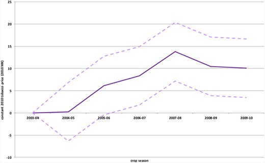
The estimations, reported in Table 2, document the results of the estimation of the dose – response function based on the GPS. The interpretation of the coefficients in the table is complicated due to reduced form nature of propensity scores and the use of a flexible specification of the dose response function. However, the figures of the dose – response function (Figure 4) are easier to digest. These figures suggest that both crop area and production are negatively correlated with distance to auction floor: a higher distance to the auction floor is associated with lower crop area and production. This outcome confirms previous difference-in-difference estimates20. Moreover, the figures suggest that crop area and production in EPAs with a short distance to auction floor (less than 60 km) have a larger response than EPAs further away from auction floors. In fact, the figures indicate that a change in distance to auction floor beyond 60 km triggers very little response.
Market access in tobacco: dose response estimations
| Dependent variable | ln (production) | ln (area) | ln (production per hectare) |
|---|---|---|---|
| (1) | (2) | (3) | |
| ln (distance to auction floor) | −0.007*** (0.0014) | −0.007*** (0.0014) | 0.0001 (0.0003) |
| GPS | −0.990*** (0.359) | −0.744** (0.349) | −0.246*** (0.070) |
| Number of observations | 1,038 | 1,038 | 1,038 |
| F (.) | (2.1035) 14.43 | (2.1035) 14.58 | (2.1035) 6.80 |
| Prob > F | 0.000 | 0.000 | 0.001 |
| Adjusted R2 | 0.0253 | 0.0255 | 0.0111 |
Notes – the table reports dose – response estimations of the introduction of a tobacco auction floor on tobacco production per hectare, using generalised propensity scores, the continuous treatment variant of propensity scores. Covariates used in constructing the generalised propensity score are rainfall, real lagged tobacco and maize price, lagged area productivity in maize and tobacco and the lagged share of maize in total crop area. The selection of variables underlying the estimation of the propensity score supports the balancing property. Estimations are based on annual data from 2003–2004 to 2009–2010 (7 years). * means significant at the 10 per cent level (p < 0.10), ** at the 5 per cent level (p < 0.05) and *** at the 1 per cent level (p < 0.01).
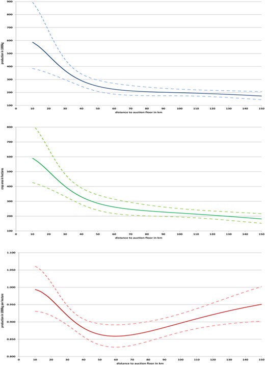
Dose – response function: impact of distance to auction floor on production (upper), crop area (middle) and area productivity (lower).
Note to figure: the dashed lines indicate the 95 per cent confidence intervals around the point estimates (the solid line)
These results give guidance on the geographical density of auction floors: a back-of-the-envelope calculation suggests scope for a doubling of the number of auction floors21. The non-linear impact is due to the GPS method. For distance to auction floor below 60 km, the distance to auction floor elasticity for production, estimated with OLS, correspond roughly with the elasticity of the dose – response estimations. The distance to auction floor elasticity for crop area, estimated with OLS, is somewhat lower compared to the elasticity of the dose – response estimations.
6. Alternative explanations and potential threats
6.1. Impact on other crops
The statistically significant impact on tobacco area, production and yield in the EPAs that are benefitting from the newly established auction floor may be a coincidental outcome that applies to all crops in these EPAs. For this reason, we have repeated the impact estimations using area, production and yield of alternative crops, notably maize, groundnuts and pulses. Maize is the key food crop and produced by virtually all households. Maize accounts for more than 50 per cent of total crop area and around 60 per cent of the Malawi food consumption diet (MoAFS and FAO). Groundnut is (partly) a cash crop like tobacco but also a food crop. Groundnut cultivation has a country-wide distribution similar to tobacco, and groundnuts are also an important source of income for farm households, although less important than tobacco. Cultivation of pulses is less widely distributed. With the exception of maize, these alternative crops are, like tobacco, high-value crops with per kg price of 4.5 to 8 times the price of maize. Since endogeneity of the intervention locations cannot be an issue for these alternative crops, we do not need to apply estimation methods that adjust for the associated bias: we can safely apply the previously used difference-in-difference specification. Estimations results are reported in Table 3.
Impact estimations with placebo crops
| Dependent variable | ln (production) | ln (crop area) | ln (production per hectare) |
|---|---|---|---|
| Crop: maize | (1) | (2) | (3) |
| ln (distance to auction floor) | −0.061 (0.093) | −0.102* (0.055) | 0.041 (0.066) |
| Number of observations | 1,318 | 1,318 | 1,318 |
| R2 | 0.866 | 0.936 | 0.787 |
| Crop: groundnuts | (1) | (2) | (3) |
| ln (distance to auction floor) | 0.140 (0.087) | 0.066 (0.085) | 0.073 (0.044) |
| Number of observations | 1,318 | 1,318 | 1,318 |
| R2 | 0.903 | 0.925 | 0.604 |
| Crop: pulses | (1) | (2) | (3) |
| ln (distance to auction floor) | 0.119 (0.04727) | 0.150 (0.108) | 0.031 (0.066) |
| Number of observations | 1,318 | 1,318 | 1,318 |
| R2 | 0.952 | 0.924 | 0.607 |
Notes – the table reports impact of distance to auction floor on maize, groundnut and pulses production, crop areas and production per hectare. Estimations are based on annual data from 2003–2004 to 2009–2010 (7 years). All estimations include EPA and year-fixed effects. All equations are estimated with OLS. Robust standard errors clustered by EPAs are given in parentheses below the coefficient. R2 = coefficient of determination and. * means significant at the 10 per cent level (p < 0.10), ** at the 5 per cent level (p < 0.05) and *** at the 1 per cent level (p < 0.01).
The table shows that the coefficients of distance to auction floor are small and statistically insignificant, or, in one case, only weakly significant. Hence, the estimation results do not support a systematic and statistically significant impact on area, production and yield, of maize, groundnuts and pulses. The hypothesis that the estimated impact on tobacco area, tobacco production and tobacco yield applies to other crops, as well, is not confirmed by the estimations. This result further strengthens our claim that improved market access – by the introduction of a new auction floor – has a positive impact on production per hectare, production and area of smallholder tobacco farmers.
6.2. Quality of the data
Researchers occasionally point at the poor quality of Malawi administrative data, mostly, however, in relation to maize production data (maize is therefore occasionally referred to as a political crop). For this reason, we have compared the EPA data from the AES-MoAFS – the data that we use for the empirical estimations – with the auction sales volume data from TCC and with tobacco information extracted from the IHS-2 from the National Statistical Office (see Appendix B). Tobacco data from different sources show discrepancies. Most discrepancies, however, have reasonable explanations22. However, a number of discrepancies merit further investigation. Since the EPAs in the districts with the largest discrepancies (Dowa, Lilongwe, Kasungu and Mchinji) partly belong to the group of EPAs that is likely to benefit from the newly introduced auction floor, this observation points to the possibility of having estimated a statistical artefact in the impact estimations, an impact that reflects the data collection process rather than a real response of tobacco growers. To investigate if the estimated impacts are statistical artefacts, we have checked the robustness of the results by omitting data from these districts.
The results reported in Appendix D show that estimates of impacts do change (which is not surprising given the key role these districts play in the identification of the impact of distance to auction floor) but remain to a large extent statistically significant and of similar size. Previous estimates of impact, hence, can be maintained.
6.3. Ceilings to expansion
Another issue concerns the presence of ceilings to expand: if all land suitable for tobacco cultivation is exhausted, there are no possibilities for further growth of tobacco production. EPAs that meet these conditions cannot be used as controls. At the level of the individual smallholder farmer, there is a variety of constraints to crop area expansion. Tobacco cultivation requires crop rotation and, hence, a minimum acreage per household (Harashima, 2008). Access to auction floors – a pre-requisite for higher prices – makes a minimum level of production and, hence, a minimum acreage necessary (Harashima, 2008). Tobacco cultivation further involves high per acre input costs, which creates another restriction to area expansion (Harashima, 2008).
Unfortunately, the EPA data do not allow to elaborate the extent of limits to area expansion along these lines. However, we can do a simple calculation based on our EPA data. Potential availability of crop area is investigated by constructing estimates of increase of total crop area and area available by substitution of other crops (see Appendix E). Under fairly reasonable assumptions, it is shown that most EPAs have potential expansion opportunities for tobacco cultivation higher than 100 per cent of existing tobacco area. The EPAs with less potential expansion opportunities still have a minimum opportunity for expanding tobacco area of 20 per cent. These calculations indicate that average expansion opportunities of crop area of non-intervention EPAs, expressed in terms of existing tobacco area, are no effective restriction.
7. Summary and conclusion
We have investigated the impact of improved market access for a typical developing country export crop on the smallholder’s decisions on cultivated area and production. For this purpose, we have used Malawi tobacco area and production data and exploited the introduction of an additional tobacco auction floor for identification. Estimations are based on annual data by EPAs, 198 in total, covering the whole of Malawi, for a period of seven years, from 2003 to 2009. Tobacco is the most important cash crop in Malawi, grown in all districts of Malawi, exclusively sold on auction floors and subsequently entirely exported. There are four tobacco auction floors (Limbe (close to Blantyre), Kanengo (close to Lilongwe), Mzuzu and Chinkhoma), of which the one in Chinkhoma has started operations in 2004. The estimation results support a statistically significant positive impact of the introduction of the new auction floor, on tobacco area and tobacco production. As the increase in production is larger than the increase in area, area productivity increases. The increase in area productivity suggests intensification of tobacco cultivation by existing growers. The impact of the introduction of the Chinkhoma auction floor is confirmed with generalised propensity matching, a matching technique that is especially designed for the case of continuous treatment. Alternative explanations for and threats to the estimated impact (estimated impact applies to all crops, common trend assumption, restrictions to expansion in non-intervention locations and the measured impact is the result of poor quality of the data) could all be rejected. The outcome points to substantial welfare benefits for smallholders when marketing infrastructure is improved and more auction floors are introduced.
Acknowledgements
I would like to thank Eric Bartelsman, Hans Binswanger, Frank Bruinsma, Chris Elbers, Christopher Gilbert, Peter Lanjouw, Thea Nielsen, Menno Pradhan, Asger Moll Wingender, Bram Thuysbaert, and conference participants in Götenborg, Sweden (Nordic Conference in Development Economics, 2012), Dakar, Senegal (PEGNet, 2012), Université Dauphine, Paris, France (DIAL, 2013), Milan (ICAE, 2015), colleagues of VU-University Amsterdam and various anonymous journal reviewers for useful comments and discussions on previous versions of this paper. Errors and omissions in the current paper are the responsibility of the author. I also would like to thank Hans Quene for skilful assistance in constructing the data and variables.
Footnotes
Food crops may also be sold on the market and, hence, are not necessarily or exclusively used for subsistence.
Promotion of either food crops or commercial crops is also at the heart of policy discussions on economic growth and development (see e.g. Harrigan, 2003, 2008).
Critical and diverging views on the role of smallholder agriculture in economic development of Collier and Dercon (2014) and Foster and Rozenschweig (2017).
The subsistence farming trap is driven by transaction costs and price volatility. High transaction costs and high risks due to volatility of output and input prices move farmers away from the market both for purchasing inputs and selling their produce. This generates low-input and low-productivity farming, low technological progress and weak responses to market prices. This development, in its turn, weakens the incentives for market participation.
An auction floor is the physical location (building where the auction takes place, storage of tobacco, parking lots for trucks, administrative offices for recording sellers, buyers and transactions, after-sales processing units, etc.), and an auction is the actual trading between sellers and buyers that takes place on predetermined hours and during a specified period of the year.
The following quote (from Prowse and Moyer-Lee, 2014) characterises this negative status: `By the early 2000s, most donor agencies had formally distanced themselves from the (tobacco) sector. It appears that the Framework Convention on Tobacco Control, tobacco’s reputation as a pariah crop and lobbying from producers in the US led donors to disengage. A good example comes from a senior UK DFID employee, who, when asked about the backbone of the Malawian economy, stated “we do not do tobacco”. ' The current study measures how farmers respond if market access improves: tobacco is instrumental to this objective. This study is not intended to promote tobacco consumption, to support cigarette manufacturers or to deny adverse health impacts of tobacco use.
This section draws on various studies that extensively describe history, structure and institutions of the Malawi tobacco sector (Kydd and Christiansen, 1982; Orr, 2000; Diagne and Zeller, 2001; Jaffee, 2003; World Bank, 2004; Poulton et al., 2007; Tchale and Keyser, 2010; Chirwa, 2011).
Burley tobacco is a light air-cured tobacco used primarily for cigarette production. Western-type tobaccos grown in Malawi are flue-cured tobacco (also known as Virginia), NDDF and SDDF (northern and southern division dark fired, respectively). These latter types are smoke and fire dried and aged in curing barns, and thereby more capital and processing intensive relative to burley tobacco.
Since all tobacco exported from Malawi is required to be sold at auction, unit values and sales volume at auctions are reasonable indicators of average Malawian market prices and aggregate production, despite small quantities of tobacco sourced from Zambia and Mozambique or illegally exported (see e.g. Koesteret al.,2004). Note, however, that empirical estimations in this study are based on data from the MoAFS (AES) and not from the Tobacco Control Commission.
In this context, it is an open question as to whether the interests of smallholder tobacco growers are well served by the operations and investment decisions of AHL.
Tobacco is planted from October to November, and harvested from January to March.
See weekly reports from TCC (only available for the period from 2001 to 2006). Since 2006–largely beyond the period of study – the role of direct trade has increased, presumably because of compliance and traceability requirements (see Moyer-Lee and Prowse, 2015).
The EPA data cover all land area of Malawi relevant for agriculture: national parks and lakes are excluded.
Note that including time-fixed effects in the estimations partially absorbs shocks and trends in road infrastructure.
We use the centroid of an EPA to measure distance from tobacco farmer to auction floor. Unfortunately, we do not know the exact locations of the tobacco farmer(s) within the EPA. Therefore, we have assumed, to stay on the safe side, that farmers may be located in the EPA closer to the new auction floor than the centroid of the EPA: the question is how do we measure this? We have approximated this with the square root of the EPA land area.
Data sources and data construction are explained in detail in Appendix A.
Because of the many missing observations and its constructed nature (see Appendix A), we have less confidence in event plots for tobacco farm gate prices.
Similar to the event estimations, we have estimated impact using a binary impact variable, a variable that takes the value of one if the distance to auction floor decreases and zero elsewhere. The estimations measure the average impact of the reduction in distance to auction floor and indicate increases in production, crop area and yield of 33, 16 and 22 per cent, respectively, all statistically significant (results available from the author). These outcomes compare reasonably well with other studies on improved market access (see, for example Goyal, 2010).
We employed the STATA commands gpscore and doseresponse. Output reported in this section is based on these commands.
The figures of the dose – response function, shown in Figure 4, indicate a negative response of production, crop area and production per hectare, and this negative relationship is stronger below 60 km. Elasticities calculated on the basis of the below-60 km slope of these lines (take two points in each figure and calculate elasticities on the basis of changes and means) come close to the coefficients of the difference-in-difference estimates reported in Table 1.
The maximum road distance for which a large impact is measured is approximately 60 km. An area with a radius of 60-km road distance is, hence, π × (60)2 = 11,309.7 km2. Malawi has a land area of 94,280 km2. Hence, there is scope for 94,280/11,309.7 = 8.3 auction floors to optimally service smallholders. If we keep in mind that road distance is, on average, 25 per cent higher than the distance measured `as the crow flies' the number of auction floors increases further.
Explanations are, for example, the distinction between smallholders and estates, and burley tobacco and other tobaccos, storage by farmers and lags in sales, measurement errors in recording, (illegal) cross border trade, etc.
Strictly, we should also analyse if availability of labour and tobacco cultivation expertise is a restriction to growth of tobacco production in the control EPAs. This is particularly relevant since tobacco cultivation is considered labour intensive. Unfortunately, we are unable to implement such an analysis. Hence, we have implicitly assumed no restrictions on these grounds.
Congestion at auction floors – particularly at the Lilongwe auction floor – arises because of bales with non-tobacco-related materials and disagreements over auction prices, which lead to suspension of market activities. Consequently, clearance of auction floors is slow and results in queuing of trucks outside the auctions for as long as 4 weeks. This often increases transport rates of drivers, and thereby increases costs for tobacco growers.
References
Appendix A: Data used, data sources and variable construction
Annual data of smallholder agricultural production and crop area at the level of EPAs, for the years from 2003/2004 to 2009/2010, are from the AES-MoAFS. All production and area data pertain to smallholders and exclude estates. An EPA reclassification in Salima and Nkothakotha districts has made a number of before-re-classification EPAs different from their equally named after-reclassification EPAs. Therefore, after reclassification observations, the shortest series have been removed.
Monthly farm gate prices for tobacco are also sourced from the AES-MoAFS, and are observed for close to 50 locations, scattered over Malawi. However, these series are not complete. Around 43 per cent of the tobacco farm gate price data used in the empirical work (annuals, seasonal averages) are directly taken from the data sources. The remaining observations are constructed by calculating a location-specific (average) share of farm gate prices in national auction prices (TCC) and imputing these values to fill up the missing observations. Time series auction price data are unfortunately only available at the national level. Tobacco farm gate prices expressed as a share of the auction prices are 35.2 per cent on average (median: 33.2 per cent). This compares reasonably well with other sources (Koester et al., 2004). All price data are attributed on the basis of proximity of markets to EPAs. In some cases, this involved averaging over various locations (triangulation). Data on farm gate maize prices are also from the AES-MoAFS. These monthly series are available for close to 60 locations, but in contrast with burley tobacco farm gate prices, the maize price series are much more complete: around 84 per cent of the maize farm gate price data are directly taken from the data source. The remaining missing observations are constructed using nearby prices. Like tobacco prices, the maize price series are attributed to EPAs on the basis of the minimum distance of the geographical location of farm gate prices to the EPA. Groundnut prices are market prices – due to limited availability of farm gate prices and in contrast with tobacco and maize prices – and available for over 70 markets. All prices are deflated with the Malawi consumer price index for rural areas.
Annual data on rainfall in mm are from around 30 meteorological stations and supplied by the Department of Climate Change and Meteorological Services, Blantyre. Again, we exploit the distance between meteorological stations and EPAs to find the rainfall series that is relevant for a specific EPA. The distance to the nearest weather station is, in most cases, less than 20 km. If more than one weather station is nearest to an EPA, we calculated the average between the nearest weather stations (triangulation).
Data on the number of households by EPA for one year (2007–2008) are from the MoAFS. Combined with district data on average household size and population, we have constructed EPA population series from 2003–2004 to 2009–2010. Population by district data are census based and from the NSO. The EPA population series is used to construct EPA population density (EPA population in numbers by EPA land area in km2) or, alternatively, per capita area. EPA land area is constructed on the basis of a map of EPAs and made consistent with data on district area (source: www.geohive.com). The size of EPAs in km2 pertains to land area (and hence excludes large lakes, like for example Lake Chilwa). The population density series varies both over time and between EPAs (but, naturally, the variation over time is limited). For the construction of an agglomeration index and distance to cities and towns, we use a 1998 and 2008 listing of population of Malawi cities and towns, taken from National Statistical Office of Malawi.
The larger the population of the city or town and the shorter the distance to the city or town, the higher the index. The agglomeration index reflects the degree of embedding of an EPA in the network of cities and towns. The higher this degree, the lower are transaction costs, and hence, we expect a positive relationship with tobacco production per hectare, production and area. It also represents the requirement to have access to market, since cash crop growers need to rely more on markets for their food purchases, for purchases of manufactured goods and for purchases of inputs (De Janvry and Sadoulet, 2006)). Summary statistics of the EPA level data are presented in Table A1.
Summary statistics of EPA level variables (annuals, from 2003–2004 to 2009–2010)
| Variable | Unit | Mean | Median | Standard deviation | Maximum | Minimum |
|---|---|---|---|---|---|---|
| Tobacco production | 1,000 kg | 735 | 293 | 1,041 | 7,058 | 0 |
| Tobacco area | ha | 799 | 339 | 1,071 | 6,073 | 0 |
| Tobacco yield | Ton/hectare | 0.941 | 0.925 | 0.322 | 2.652 | 0.233 |
| Maize production | 1,000 kg | 13,389 | 11,138 | 9,668 | 68,810 | 214 |
| Maize area | ha | 8,376 | 7,965 | 4,371 | 32,100 | 130 |
| Maize yield | Ton/hectare | 1.631 | 1.571 | 0.709 | 6.949 | 0.189 |
| Groundnut production | 1,000 kg | 1,196 | 711 | 1,412 | 12,489 | 1 |
| Groundnut area | ha | 1,364 | 1,020 | 1,221 | 9,384 | 4 |
| Groundnut yield | Ton/hectare | 0.789 | 0.770 | 0.300 | 3.239 | 0.019 |
| Pulse production | 1,000 kg | 1,105 | 1,879 | 2,158 | 16,432 | 2 |
| Pulse area | ha | 3,053 | 2,093 | 2,934 | 16,340 | 3 |
| Pulse yield | Ton/hectare | 0.593 | 0.577 | 0.221 | 2.391 | 0.024 |
| All crops’ area | ha | 16,571 | 14,979 | 8,177.9 | 50,833 | 1,090 |
| Tobacco price | MK/kg | 55.6 | 45.0 | 30.9 | 190.0 | 19.2 |
| Maize price | MK/kg | 18.3 | 15.3 | 9.0 | 44.8 | 6.0 |
| Groundnut price | MK/kg | 114.0 | 124.0 | 51.6 | 338.5 | 35.6 |
| Chemical fertilizer | kg/hectare | 0.114 | 0.101 | 0.075 | 0.626 | 0 |
| Rainfall | mm | 943.9 | 901.3 | 263.2 | 2,151 | 378 |
| Population | n | 70,069 | 61,150 | 48,371 | 416,052 | 3,402 |
| Land area | km2 | 470.1 | 406.5 | 241.8 | 1,201.0 | 121.2 |
| Population density | n/km2 | 189.0 | 139.2 | 162.3 | 1,408.1 | 7.7 |
| Agglomeration index | Index | 17.0 | 15.2 | 9.6 | 79.2 | 4.0 |
Note: price and rainfall data are originally by a limited number of markets/weather stations and attributed to EPAs (see explanation above); chemical fertiliser is kilogram of urea and NPK per hectare of (tobacco+maize) area.
For descriptive purposes, we use one year of auction transaction data (2009, a total of around 62,000 transactions), which were kindly made available by the TCC. Each transaction contains information on type of tobacco, number of bales, volume in kg, values in US$, district of origin and club. Also for descriptive purposes, we use annual aggregate times series data on the tobacco sector from TCC, posted on TCC website (www.tccmw.com).
Appendix B: Comparison of tobacco data by source: AES-MoAFS, IHS (NSO) and TCC*
Aggregate annual production (AES-MoAFS) versus sales volume (TCC).
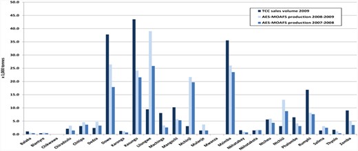
Production (AES-MoAFS) versus sales volume (TCC) by district, 2009.

Production (AES-MoAFS) versus production (IHS-2) by district, 2003–2004.
*AES-MoAFS: Agro-Economic Survey, Ministry of Agriculture and Food Security; TCC: Tobacco Control Commission; IHS: Integrated Household Survey; NSO: National Statistical Office.
Appendix C: Event study plot for farm gate prices
Figure C1 shows the plot of the event estimation of tobacco farm gate prices and is similar to the plots in the main text (Figure 3). Likewise, we estimated
Impact of lower transport costs on farm gate tobacco prices.
Note: we estimated
Appendix D: Are poor quality data driving estimated impacts?
Market access in tobacco: omitting observations of specific district
| Dependent variable | ln (production) | ln (area) | ln (production per hectare) |
|---|---|---|---|
| District omitted: Kasungu | (1) | (2) | (3) |
| ln (distance to auction floor) | −0.937*** (0.340) | −0.376* (0.226) | −0.561* (0.288) |
| Number of observations | 1,144 | 1,144 | 1,144 |
| R2 | 0.939 | 0.958 | 0.510 |
| District omitted: Lilongwe | (1) | (2) | (3) |
| ln (distance to auction floor) | −0.889** (0.360) | −0.340 (0.236) | −0.550* (0.308) |
| Number of observations | 1,026 | 1,026 | 1,026 |
| R2 | 0.937 | 0.956 | 0.514 |
| District omitted: Mzimba | (1) | (2) | (3) |
| ln (distance to auction floor) | −0.920** (0.465) | −0.085 (0.207) | −0.835* (0.448) |
| Number of observations | 1,033 | 1,033 | 1,033 |
| R2 | 0.941 | 0.961 | 0.517 |
| District omitted: Mchinji | (1) | (2) | (3) |
| ln (distance to auction floor) | −0.894*** (0.293) | −0.485** (0.235) | −0.409** (0.178) |
| Number of observations | 1,117 | 1,117 | 1,117 |
| R2 | 0.938 | 0.456 | 0.515 |
Notes–the table reports estimates of impacts of distance to auction floor on tobacco production, crop area and production per hectare. The robustness of the basic estimation of Table 1 is tested by omitting observations from specific districts. Estimations are based on annual data from 2003–2004 to 2009–2010 (7 years). All estimations include EPA and year fixed effects. All equations are estimated with OLS. Robust standard errors clustered by EPAs are given in parentheses below the coefficient. R2 = coefficient of determination. *P < 0.10, **P < 0.05, ***P < 0.01.
Appendix E: Is crop area available for tobacco cultivation effectively limited?
Potential availability of crop area can be investigated: EPA data on crop area are available for all major crops and for this exercise, we distinguish crop area for tobacco, maize and other crops, where ‘other crops’ are an aggregate of rice, groundnuts, pulses, cassava, sweet potatoes, cotton, sorghum and millet. The data underscore the overwhelming importance of maize, with an average share of around 50 per cent of total crop area. Note that the average tobacco share in total crop area is less than 5 per cent (median less than 2.5 per cent). Expansion of tobacco crop area occurs either through expansion of total crop area or through substitution with other crops. We assume that the potential for expansion of total crop area may be approximated with the gap between the maximum total crop area realised over the years 2003/2004 to 2009/2010 and actual total crop area, both by EPA. Hence,
Appendix F: TCC auction floor transaction data for the 2009 marketing season
For descriptive purposes, we have exploited a TCC data set for 2009 auction floor transactions. Table 1 shows the number of transactions by type and by auction floor in these data. Summary statistics on sales volume by district and auction floor are documented in Table F3.

Unit values by auction floor.
Source: estimations based on TCC 2009 auction floor transaction data. Unit values are sales value (in US$) divided by sales volume (in kg)
Transactions by type and auction floor, 2009 (number of transactions, row and column share in per cent)
| Type | Auction floor | ||||
|---|---|---|---|---|---|
| Chinkhoma | Lilongwe | Limbe | Mzuzu | Total | |
| Burley | 10,602 | 15,583 | 14,909 | 18,121 | 59,215 |
| 17.9 | 26.3 | 25.2 | 30.6 | 100 | |
| 95.3 | 95.3 | 98.9 | 94.1 | 95.8 | |
| Flue | 443 | 579 | 149 | 714 | 1,885 |
| 23.5 | 30.7 | 7.9 | 37.9 | 100 | |
| 4.0 | 3.5 | 1.0 | 3.7 | 3.1 | |
| NDDF | 75 | 192 | 20 | 424 | 711 |
| 10.6 | 27.0 | 2.8 | 59.6 | 100 | |
| 0.7 | 1.2 | 0.1 | 2.2 | 1.2 | |
| Total | 11,120 | 16,354 | 15,078 | 19,259 | 61,811 |
| 18.0 | 26.5 | 24.4 | 31.2 | 100 | |
| 100 | 100 | 100 | 100 | 100 | |
Source: TCC.
Premia by auction floor
| Dependent variable: unit value (transaction value/transaction quantity) | ||||
|---|---|---|---|---|
| Sample: type size producer | Burley all | Burley small (<1,717 kg) | Burley large (>6,356 kg) | Flue all |
| Chinkhoma | −0.103*** (0.008) | −0.156*** (0.023) | −0.081*** (0.010) | 0.571*** (0.095) |
| Lilongwe | −0.201*** (0.008) | −0.200*** (0.023) | −0.207*** (0.010) | 0.364*** (0.095) |
| Limbe | −0.108*** (0.009) | −0.136*** (0.025) | −0.116*** (0.013) | 0.139 (0.213) |
| Mzuzu | — | — | — | — |
| constant | 1.722*** (0.005) | 1.765*** (0.015) | 1.709*** (0.007) | 2.097*** (0.060) |
| adjusted R2 | 0.049 | 0.021 | 0.003 | 0.298 |
| n | 59,213 | 19,738 | 19,738 | 1,885 |
Source: TCC 2009 auction floor transaction data and refer to the 2009 tobacco marketing season; unit values are sales value (in US$) divided by sales volume (in kilograms); all equations are estimated with producer fixed effects. Smaller (larger) producers pertain to the one-third lower (upper) part of the transaction distribution. Standard errors in brackets next to the coefficient are clustered by district. *P < 0.10, **P < 0.05, ***P < 0.01.
Sales volume by tobacco auction floor* and by district of origin, 2009
| District | Sales volume (in 1,000 kg) | Per district distribution over floors in per cent | Per floor distribution over districts in per cent | ||||||||||||
|---|---|---|---|---|---|---|---|---|---|---|---|---|---|---|---|
| MZZ | CNK | LIL | LMB | Total | MZZ | CNK | LIL | LMB | Total | MZZ | CNK | LIL | LMB | Total | |
| Chitipa | 2,991 | 0.1 | 118 | 0.1 | 3,110 | 96.2 | 0.0 | 3.8 | 0.0 | 100 | 4.3 | 0.0 | 0.2 | 0.0 | 1.5 |
| Karonga | 12,288 | 16 | 24 | 4.0 | 1,272 | 96.5 | 1.3 | 1.9 | 0.3 | 100 | 1.8 | 0.1 | 0.0 | 0.0 | 0.6 |
| Rumphi | 16,383 | 469 | 4.0 | 16,856 | 97.2 | 2.8 | 0.0 | 100 | 23.6 | 1.7 | 0.0 | 8.2 | |||
| Nkhata Bay | 1,530 | 3 | 2.7 | 1,535 | 99.6 | 0.2 | 0.2 | 100 | 2.2 | 0.0 | 0.0 | 0.7 | |||
| Mzimba | 34,913 | 550 | 34 | 46 | 35,543 | 98.2 | 1.5 | 0.1 | 0.1 | 100 | 50.2 | 2.0 | 0.1 | 0.1 | 17.2 |
| Nkhotakota | 472 | 568 | 29 | 403 | 1,472 | 32.1 | 38.6 | 1.9 | 27.4 | 100 | 0.7 | 2.0 | 0.1 | 0.7 | 0.7 |
| Kasungu | 9,228 | 16,737 | 16,424 | 1,139 | 43,528 | 21.2 | 38.5 | 37.7 | 2.6 | 100 | 13.3 | 60.2 | 30.1 | 2.1 | 21.1 |
| Ntchisi | 415 | 1,977 | 73 | 633 | 3,098 | 13.4 | 63.8 | 2.4 | 20.4 | 100 | 0.6 | 7.1 | 0.1 | 1.2 | 1.5 |
| Dowa | 1,361 | 5,494 | 29,337 | 1,593 | 37,786 | 3.6 | 14.5 | 77.6 | 4.2 | 100 | 2.0 | 19.8 | 53.7 | 2.9 | 18.3 |
| Mchinji | 400 | 678 | 421 | 1,580 | 3,079 | 13.0 | 22.0 | 13.7 | 51.3 | 100 | 0.6 | 2.4 | 0.8 | 2.9 | 1.5 |
| Salima | 54 | 45 | 4.9 | 1,345 | 1,450 | 3.7 | 3.1 | 0.3 | 92.8 | 100 | 0.1 | 0.2 | 0.0 | 2.5 | 0.7 |
| Lilongwe | 481 | 1,199 | 6,364 | 1,428 | 9,471 | 5.1 | 12.7 | 67.2 | 15.1 | 100 | 0.7 | 4.3 | 11.7 | 2.6 | 4.6 |
| Dedza | 4.1 | 22 | 1,733 | 629 | 2,388 | 0.2 | 0.9 | 72.6 | 26.3 | 100 | 0.0 | 0.1 | 3.2 | 1.1 | 1.2 |
| Ntcheu | 7.4 | 4.7 | 13 | 5,583 | 5,608 | 0.1 | 0.1 | 0.2 | 99.5 | 100 | 0.0 | 0.0 | 0.0 | 10.2 | 2.7 |
| Mangochi | 4.8 | 1.8 | 10,225 | 10,232 | 0.0 | 0.0 | 99.9 | 100 | 0.0 | 0.0 | 18.6 | 4.9 | |||
| Machinga | 2.4 | 1.5 | 2.2 | 8,050 | 8,056 | 0.0 | 0.0 | 0.0 | 99.9 | 100 | 0.0 | 0.0 | 0.0 | 14.7 | 3.9 |
| Balaka | 1.6 | 0.3 | 1,080 | 1,082 | 0.1 | 0.0 | 99.8 | 100 | 0.0 | 0.0 | 2.0 | 0.5 | |||
| Zomba | 10 | 2.1 | 9,015 | 9,027 | 0.1 | 0.0 | 99.9 | 100 | 0.0 | 0.0 | 16.4 | 4.4 | |||
| Mwanza | 48 | 48 | 100.0 | 100 | 0.1 | 0.0 | |||||||||
| Blantyre | 5.9 | 3.0 | 3.3 | 390 | 402 | 1.5 | 0.8 | 0.8 | 96.9 | 100 | 0.0 | 0.0 | 0.0 | 0.7 | 0.2 |
| Chiradzulu | 13 | 11 | 6.7 | 2,071 | 2,102 | 0.6 | 0.5 | 0.3 | 98.6 | 100 | 0.0 | 0.0 | 0.0 | 3.8 | 1.0 |
| Phalombe | 0.4 | 3.2 | 6,429 | 6,433 | 0.0 | 0.0 | 99.9 | 100 | 0.0 | 0.0 | 11.7 | 3.1 | |||
| Mulanje | 0.7 | 1,441 | 1,442 | 0.1 | 99.9 | 100 | 0.0 | 2.6 | 0.7 | ||||||
| Thyolo | 0.0 | 1,714 | 1,714 | 0.0 | 100.0 | 100 | 0.0 | 3.1 | 0.8 | ||||||
| Chikwawa | 0.0 | 0.0 | 0.0 | 19 | 19 | 0.0 | 0.0 | 0.0 | 100.0 | 100 | 0.0 | 0.0 | |||
| Total | 69,504 | 27,788 | 54,588 | 54,871 | 206,750 | 33.6 | 13.4 | 26.4 | 26.5 | 100 | 100 | 100 | 100 | 100 | 100 |
Source: transaction data for 2009 from the TCC, Malawi (around 60,000 observations); * CNK = Chinkhoma; LIL = Lilongwe (Kanengo); LMB = Limbe; MZZ = Mzuzu. Notes – Districts of origin and auction floors, ordered from north to south. Regions (north, central and south) are distinguished by shading.
With the transaction data, we can show if burley tobacco fetches a premium if sourced from a specific district, or if auctioned at a specific auction floor. Finding premium by auction floor exploits the panel character of the data: a substantial number of sellers have multiple sales on different auction floors. It should be noted that we only have limited information on potential explanations of price differences. There is, for example, no information on quality grades of tobacco, congestion at auction floors24 and delays in payment (which are believed to be considerable, important to farmers, but not recorded). These circumstances may affect prices realised on auction floors.
Table F2 and Figure F1 indicate that the Mzuzu auction floor yields the highest unit values for burley tobacco, while for the Lilongwe floor burley unit, values are lowest. Comparing averages indicates that Mzuzu auction floor prices are around 13 per cent higher than Lilongwe auction floor prices. Furthermore, large producers and flue-cured tobacco appears to fetch a premium on the Chinkhoma auction floor. Explaining differences in unit values by floor is beyond the scope of the current exercise. Apart from composition and quality, constraints to arbitrage are likely to play a role.
The above result averages over origins. One can run similar estimations, regressing unit values on districts of origin, to find if specific origins fetch a premium. Results for burley tobacco – shown in Figure F2–indicate higher unit values for the northern districts and lower unit values for the southern districts, with a maximum difference of 25 per cent. Again, this may be further disaggregated by auction floor, in order to find district premium that differ by type or auction floor: these results (not shown to save space) suggest that district differences nearly fully disappear at the level of different auction floors, which makes support for a ‘district of origin premium’ not strong.
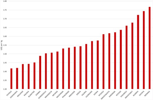
Unit values by district of origin.
Source: estimations based on TCC 2009 auction floor transaction data. Unit values are sales value (in US$) divided by sales volume (in kg)
The question arises if there is any correlation between the size of the individual seller on the auction floor – measured by the total volume sold on auction floors by an individual farmer, a farmers’ club or an estate – and the level of the price. We measure this by running a non-parametric estimation of unit values on size (classes): specifically by having distributed all transactions in 10 classes, equally sized in number of transactions, where the classes are constructed by ranking transactions by the total volume of sales of an individual seller. Note that each seller may have different transactions on different auction floors. The result of this exercise – as shown in Figure F3–indicates 4–11 per cent higher prices for smaller sellers (the darker bars in Figure F3), and this is specifically the case for the Lilongwe, Limbe and Mzuzu auction floors, but reversed on the Chinkhoma auction floor.
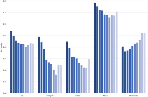
Unit values by size of seller.
Source: estimations based on TCC 2009 auction floor transaction data. Unit values are sales value (in US$) divided by sales volume (in kg). Transactions are ranked into 10 equally sized volume of transaction classes: the darker (lighter) the bar, the smaller (larger) the volume of the transaction
