


Abstract
I measure the economic effects of greenbelts that prohibit new construction beyond a predefined urban fringe and therefore act as urban growth boundaries. I focus on England, where 13% of the land is designated as greenbelt land. I provide reduced-form evidence and estimate a quantitative equilibrium model that includes amenities, housing supply, a traffic congestion externality, agglomeration forces, productivity and household location choices. Greenbelt policy generates positive amenity effects, but also strongly reduces housing supply. I find that greenbelts increase welfare because amenity effects are sufficiently strong. At the same time, however, greenbelts decrease housing affordability by limiting housing supply.
In most countries, urban growth leads to increasing pressure on developable land in and around cities. Many cities regulate urban development by imposing a range of constraints on, e.g., building height or type of land use. Local governments also frequently restrict the expansion of urban areas to prevent urban sprawl. These urban growth boundaries or greenbelts reduce land available for development at the urban fringe. Many US cities, such as Portland (OR), Miami, Minneapolis Saint-Paul and San Jose (CA), have urban growth boundaries (UGBs), and similar restrictions can be found in many other countries (e.g., Austria, Canada, China, France, Germany, Iran, the Netherlands, New Zealand, Norway and South Korea). I focus on England, where greenbelts are important as they cover approximately |$13\%$| of the total area and surround most larger cities.
Land-use regulation does not necessarily lead to welfare losses, because constraints may reduce negative land-use externalities and frictions associated with development. Greenbelt policy indeed intends to protect agricultural land and secure amenity benefits from open space (Brueckner, 2001). At the same time, when regulatory constraints are too strict, regulation may lead to substantial economic losses. Thus, economists have argued that greenbelt policy should be relaxed to mitigate the ‘housing affordability crisis’ because restrictions on housing supply lead to potentially strong price increases (Cheshire, 2014; Economist, 2017). Despite the potentially large impacts of greenbelts on the growth of cities and housing markets, to the best of my knowledge, no study has yet attempted to evaluate the welfare effects of greenbelt policy.
This study therefore seeks to measure the effects of greenbelt policy on the spatial distribution of economic activity. To do this, I first use data on the location of all dwellings in England. It appears that |$37\%$| of dwellings lie within 1 km of greenbelt land while |$2\%$| are on greenbelt land. I further exploit data on more than 10 million housing transactions between 1995 and 2017. Given information on the exact location, I can identify for each dwelling the share of greenbelt land in its vicinity. Furthermore, I use data at the middle-layer super output area (MSOA) level (which has on average a working population of around 3,800) on commuting flows and the locations of individuals and their workplaces.
The first aim of this paper is to identify the reduced-form supply and amenity effects of greenbelt land. The supply effect captures the reduction in the supply of housing in greenbelts. The amenity effect refers to the increased attractiveness of a location due to better access to green space. Estimates of these effects are potentially biased, as greenbelts are located on the outskirts of cities, where land is usually cheaper. Hence, houses close to greenbelts tend to be larger and may have gardens. To address omitted variable bias, I pursue two identification strategies. First, I exploit the fact that greenbelt boundaries in England have hardly changed since their imposition in the 1970s. I gather data on approved and proposed greenbelt land in 1973 and explain variation in prices and densities in those areas. Alternatively, as concerns may arise that the selection process of greenbelts is correlated to unobserved locational endowments, I only select areas close to greenbelt boundaries and apply spatial differencing in the spirit of Turner et al. (2014). I improve on this strategy by only including data on one side of the border so as to avoid discrete differences in housing and neighbourhood characteristics at the greenbelt border.
The local supply and amenity effects of greenbelts are only one part of the story. The substantial reduction in the supply of developable land close to cities will also influence the spatial equilibrium, resulting in a different spatial distribution of production, implying agglomeration effects. These effects are potentially relevant because residents have to commute to work. Moreover, workers are more productive when they are in the vicinity of other workers (Ciccone and Hall, 1996; Ciccone, 2002; Arzaghi and Henderson, 2008; Combes et al., 2008; Melo et al., 2009) and because traffic congestion arises when people cluster together (Combes et al., 2019; Proost and Thisse, 2019).
To model the complex interactions of amenity, supply and agglomeration effects, I set up a quantitative spatial general equilibrium model, following Ahlfeldt et al. (2015). In this model, residents and firms compete for floor space, while workers benefit from each other’s presence due to agglomeration economies. Residents commute to workplaces, so a greater concentration of firms typically implies higher commuting costs. I extend the model of Ahlfeldt et al. (2015) in three directions:
I embed land-use restrictions in the model, as greenbelt land reduces the available land available for development at certain locations;
I allow for greenbelts to generate a higher amenity level; hence, I explicitly specify the amenity residual in Ahlfeldt et al. (2015) and estimate the spatial decay of these amenities;
I allow for mode choice and endogenous travel times of road travel, i.e., for traffic congestion close to the workplace. Several papers show that UGBs affect the congestion level in a city and therefore have welfare implications through the potential reduction of congestion externalities (see Kanemoto, 1977; Arnott, 1979; Pines and Sadka, 1985; Anas and Rhee, 2007; Brueckner, 2007).
Using the recursive structure of the model, together with the identification strategies to identify the amenity and supply effects outlined above, I estimate (rather than calibrate) the structural parameters of the model.1
In contrast to Ahlfeldt et al. (2015), I do not choose, but rather estimate the share of construction cost spend on land inputs, which appears to be important. To identify this parameter, I follow Combes et al. (2021) in using the first-order condition for profit maximisation with respect to building capital and relying on variation in systematic determinants of demand for real estate across space. To identify the parameters related to agglomeration and congestion forces, I first propose a standard identification strategy using historic instruments. Alternatively, I use spatial instruments using exogenous characteristics of faraway locations, following Bayer and Timmins (2007). Given that one may question these instruments’ ability to identify causal spillover effects, I also provide analyses in which the instruments are only ‘plausibly exogenous’ (Conley et al., 2012).
I show that greenbelt policy has a small positive welfare effect given the structural parameters obtained in the preferred specifications. The income reduction if greenbelts were to be removed is |$1.4\%$|, which amounts to approximately £9 billion a year. Whether residents benefit from greenbelts critically depends on two parameters. First, it depends on the elasticity of building production with respect to non-land inputs. When this exceeds around 0.55, I find positive effects of greenbelts. For high values of this elasticity, it is cheaper to transform land into buildings, meaning that the reduction in land due to greenbelt policy is less costly. Second, I show that the benefits of greenbelts for residents dissipate once greenbelt amenities cease to exist. This shows that greenbelt amenities are key in understanding why welfare effects of greenbelts can be positive. Interestingly, agglomeration economies do not seem to be crucial, which is in line with Kline and Moretti (2014), who argued that agglomeration economies are a localised market failure that cancels out in the aggregate. Furthermore, I show that greenbelts lead to higher real estate prices: in cities like London, Birmingham and Manchester, property prices drop by 5%–|$20\%$| when greenbelts are removed. Hence, although greenbelts increase overall welfare, they inevitably and strongly reduce housing affordability.
The welfare measure used in this paper arguably does not include all possible general equilibrium effects. Still, to the extent I do not include potential other benefits of greenbelts (e.g., reductions in pollution, or city-wide amenity increases) that spill over to people living in cities, the estimate of welfare gains of greenbelts can be considered as an underestimate.
This paper contributes to the literature in several ways. Most previous studies on the effects of land-use regulation concentrate on housing supply restrictions and indicate that supply constraints are associated with increasing housing costs, a strong reduction in new construction and rapid price growth (Mayer and Somerville, 2000; Glaeser et al., 2005; Green et al., 2005; Ihlanfeldt, 2007). This effect is particularly pronounced for cities in England, in which land-use regulation is highly restrictive (Hilber and Vermeulen, 2016).2 Other evidence for England by Cheshire et al. (2018) shows that land-use restrictions may also lead to higher vacancy rates and longer commutes. Glaeser and Ward (2009) found that local constraints in Boston (i.e., within a city) do not increase the price of land because of close substitutes. At the same time, they found that density levels are too low from a welfare perspective. Koster et al. (2012) found that the costs of regulation for homeowners or developers (so-called ‘own-lot effects’) may be substantial (up to |$10\%$| of the housing value). Turner et al. (2014) evaluated the own-lot and amenity effects of land-use regulation in the United States. Own-lot effects appear to be substantial, but they did not find evidence for amenity effects, which suggests that land-use regulation has negative welfare consequences in that context.3 Harari (2020) showed that, for India, the shape of cities matters. Less compact cities, which imply longer within-city travelling distances, are associated with a lower quality of life. In India, land-use regulation typically promotes less compact developments and therefore further reduces urban accessibility and welfare.
This paper also relates to research that measures the local benefits of open space. Some studies have specifically focused on reduced-form house price impacts of greenbelt land. An early study by Correll et al. (1978), for instance, reports that properties near greenbelt land are generally more expensive, but the reported effects are unlikely to be causal. Jun (2006) showed no evidence of a significant difference between housing prices inside and outside the UGB, confirming that these areas are part of a single housing market. By contrast, Grimes and Liang (2009) found that land just inside the UGB in Auckland, New Zealand, is valued at approximately 10 times that of land just outside the boundary, which is the result of better redevelopment opportunities within the urban limit. While these reduced-form estimates show that UGBs are relevant, they do not provide clear implications as to whether greenbelts increase or decrease welfare. Other studies focus explicitly on the measurement of the benefits of open space. Bolitzer and Netusil (2000), for example, found that living close to green space increases property values by maximally |$5\%$|, while Irwin (2002) found that a hectare of farmland in the vicinity increases property values by |$0.75\%$|. Anderson and West (2006), however, found that the value of proximity to open space is higher in dense neighbourhoods. Geoghegan (2002) showed that open space labelled as ‘permanent’ increases nearby residential land values over three times as much as an equivalent amount of ‘developable’ open space. This may explain why I find somewhat strong effects of greenbelt land on house prices, as greenbelt land is non-developable. I note that none of the papers provides data on general equilibrium effects, such as the effects of commuting and housing supply.
Finally, this paper contributes to a mostly theoretical literature on the effects of urban growth boundaries on commuting—more specifically, whether UGBs can be a second-best policy to reduce congestion externalities. Early papers by Kanemoto (1977), Arnott (1979) and Pines and Sadka (1985) show that a not-too-stringent UGB is a second-best policy for congestion tolls when traffic congestion is unpriced. However, these papers assume that all jobs are exogenously located in one urban centre. Anas and Rhee (2007) showed that with cross-commuting, boundaries of any stringency can be inefficient even when tolls shrink cities, as boundaries do little to reduce inefficient commuting from the suburb to the city centre. Brueckner (2007) corroborated this conclusion, finding that greenbelts may not be a useful instrument for addressing the distortions caused by unpriced traffic congestion.
The plan for the remainder of the paper is as follows. In Section 1, I explain how greenbelts were designated, introduce the datasets and provide descriptives. In Section 2, I provide reduced-form evidence for the effects of greenbelt land on dwelling density and house prices. I also provide a wealth of robustness checks. Section 3 then outlines the quantitative model, and in Section 4 I report the estimated structural parameters and discuss the different counterfactual analyses. Finally, Section 5 concludes.
1. Context, Data and Descriptives
1.1. Greenbelts in England
There is a long-standing tradition in England of restricting urban growth. In the 1920s, proposals were put forward by the London Society and the Campaign to Protect Rural England (CPRE) to prevent development in a continuous belt within 2 km of London. Then, in the 1947 Town and Country Planning Act, local authorities were for the first time allowed to take planning decisions and to incorporate greenbelt proposals in their development plans.
In 1955, Duncan Sandy, who was then the Minister of Housing, encouraged local authorities around the country to consider protecting land around cities through the formal designation of well-defined greenbelts. In a statement in the House of Commons, he wrote the following:
I am convinced that for the well-being of our people and for the preservation of the countryside, we have a clear duty to do all we can to prevent the further unrestricted sprawl of the great cities. The Development Plans submitted by the local planning authorities for the Home Counties provide for a Green Belt, some 7 to 10 miles deep, all around the built-up area of Greater London. [...]. No further urban expansion is to be allowed within this belt. [...] I am accordingly asking all planning authorities to submit to me proposals for the creation of clearly defined Green Belts, wherever this is appropriate.
Greenbelts were introduced in the two decades after 1955 around almost all of England’s big cities (London, Birmingham, Liverpool and Manchester), but also around smaller cities (e.g., Bournemouth, York, Oxford and Cambridge). Most cities that put forward proposals to designate greenbelt land had at least a population of 100,000 inhabitants at that time and therefore qualified as ‘large urban areas’. Most proposals were submitted in the late 60s and early 70s, while the final approval and exact demarcation of the greenbelt borders took place in the early 80s.4 Since the official approval of greenbelts in the early 1980s, no new greenbelts have been introduced and the total amount of greenbelt land has essentially not changed in the last 35 yr.5 Currently, greenbelts cover approximately |$13\%$| of all land in England (for comparison, built-up land covers around |$10\%$|) and should, according to the National Planning Policy Framework in 2012, offer appreciable amenities to the urban population by improving access to the open countryside, by providing opportunities for outdoor sport and recreation, and by retaining attractive landscapes close to urban areas. Land-use data from Open Street Map indicate that roughly one-third of greenbelt land is used for agriculture, while only around |$5\%$| of the land is classified as parks or recreation grounds.6 Furthermore, greenbelts were not introduced to address the problems of inner cities (such as traffic congestion and walkability), but were instead introduced to protect the countryside and, in later years, to improve access to green space for people living in urban areas. Hence, although urban planners may apply other types of regulations (such as floor-area restrictions, historic building protection, etc.), this is not part of the greenbelt policy per se.
In Figure 1, I show the 14 greenbelts in England as well as national parks and areas of outstanding natural beauty (AONBs), which do not overlap. As can be seen, greenbelts are about 10–20 km deep, as suggested by Duncan Sandy, and unmistakeably surround the large cities such as London, Birmingham and Manchester. But, at the same time, Figure 1 also shows that greenbelt land is very patchy. Because towns and settlements existed before greenbelt policy was implemented, one can observe developments in greenbelt areas and on greenbelt land. In the identification strategy employed later in the paper, I employ a border-discontinuity design based on inner and outer greenbelt borders. I define those by looking at the border of development with greenbelt land surrounding the most important cities. Hence, inner greenbelt boundaries only surround the most important cities and not the small towns and villages that are fully surrounded by greenbelt land. I refer to locations as being in ‘a greenbelt area’ when they are in between the inner and outer greenbelt boundaries, although not all land in those greenbelt areas is necessarily designated as greenbelt land (for an illustration, see Online Appendix A.1).
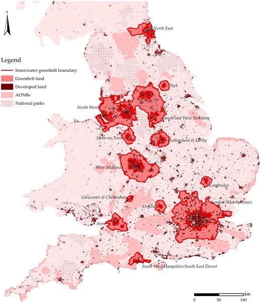
Greenbelts in England.
In the empirical analysis, I will also use the information on considered and approved greenbelt land in earlier times, i.e., in 1973. Online Appendix A.2 provides further details.
1.2. Data
1.2.1. Micro-data
I make use of four datasets on England. The first dataset pertains to the number of dwellings per postcode from the Office of National Statistics (ONS), which is based on the 2011 census (see Office of National Statistics, 2011). A postcode is very small and contains around 13 households.
Information on greenbelts in 2012 is obtained from the Department for Communities and Local Government (DCLG) (see Department for Communities and Local Government, 2012). Each local authority digitised land-use information and DCLG merged these separate datasets. I aim to identify amenity and supply effects using the boundaries of greenbelts, as these capture the actual urban containment boundaries. Hence, I determine for each greenbelt the inner and outer boundaries and calculate the distance of the centroid of each postcode to the nearest inner or outer boundary of a greenbelt. Furthermore, for each postcode, I calculate the share of greenbelt land. Because postcodes are so small, this is typically zero or one. Plus, to calculate the effects of greenbelt amenities, I calculate the share of greenbelt land within 500 m distance bands.
The third dataset contains the universe of housing transactions in England from the Land Registry between 1995 and 2017 (see H.M. Land Registry, 2017). These data provide information on the transaction price, the housing type, the date of the transaction and the ownership structure (leasehold or freehold), as well as the location at the postcode level. A disadvantage of the Land Registry data is the limited amount of information on housing characteristics. For example, the size of the property is missing.
Therefore, I merge each Land Registry transaction to energy performance certificates (EPCs) (see Department for Communities and Local Government, 2017). Since 2007, an EPC has been required whenever a home is constructed or sold. EPCs have been issued since October 1, 2008, and provide information regarding the energy performance of buildings and their characteristics, which are obtained by means of a physical inspection of the interior and exterior of the home by an independent assessor. Most notably, this provides me with the floor area of the property, the number of rooms and the energy efficiency.
My merging strategy is to sequentially match individual sales to the EPC data using the full address or a subset of the address and the date of the sale and certificate.7 Around one-third of the sales in the Land Registry remains unmatched, so I drop them from the analysis.8 I also drop some outliers and transactions that are matched to multiple EPCs (around 15%).9
Because greenbelt boundaries have hardly changed between 1995 and 2017, matching greenbelt data from 2012 to transactions in the past will imply little measurement error. Moreover, although EPCs are available from 2008 onwards, I still match transactions from the Land Registry from before 2008 to EPC, thereby assuming that housing characteristics do not change. Hence, I use the full temporal extent of the data (1995–2017).10 This leaves us with 10,070,791 sales.
1.2.2. MSOA data
For the structural model (to be introduced later), I use data at the middle-layer super output area from the 2011 census (Office of National Statistics, 2011). To obtain floor space prices, I use the above-discussed sales data from the Land Registry and EPCs and regress log prices per square metre on housing characteristics and MSOA fixed effects. I obtain floor space prices by taking the exponent of the estimated fixed effects.11 In the structural estimation, I normalise floor space prices to have a geometric mean of 1.
Furthermore, for each MSOA, I calculate the share of greenbelt land as well as the share in 1973 greenbelts. For each centroid of an MSOA, I calculate the distance to the nearest inner or outer greenbelt boundary.
From the 2011 census (Office of National Statistics, 2011), I obtain commuting flows between each of the 6,791 MSOAs, which means that I have 46,117,681 cells containing information on the number of workers commuting from home to work and by what mode. Using this information, I also calculate the total number of workers and residents by mode in each area. From Ordnance Survey I obtain information on the road network in 2012 (see Ordnance Survey, 2012). That is, I keep motorways, A roads and B roads for which I assume free-flow travel speeds of 110, 80 and 50 km/h.12 Using these network data, I calculate free-flow travel times between each MSOA pair. To obtain actual travel times, I obtain data on average speeds on major roads from the Department of Transport at the county level in 2015 (see Department of Transport, 2015). Because counties are much smaller in urban areas, this will provide a reasonable proxy for actual speeds. I then match each road to the county in which it is located and calculate actual travel times between each MSOA pair. For travel times by rail, I use data on the railway network from Open Street Map (see Open Street Map, United Kingdom, 2017). Data on London’s tube network is from Transport for London. The average speed on railways is from Cartmell (2016) and is assumed to be 57 km/h, while the average speed on tube lines from Transport for London is 33 km/h (see Transport for London, 2017).13 To calculate travel times for other modes (including walking, cycling and working from home), I use the road network, but I assume a speed on the network of 10 km/h.
In Online Appendix A.4, I provide some more details on commuting flows and show that calculated travel times are very highly correlated to actual travel times (obtained for a small subset of the data).
To construct instruments for agglomeration (to be discussed later), I gather data on the historic population at the parish level for 1931 (see A Vision of Britain, 2017). There were 11,450 parishes in 1931 (these are usually considerably smaller than MSOAs and parliamentary constituencies). For each MSOA and constituency, I calculate the share in each parish. I then assume that the population is uniformly distributed within each parish by multiplying the share of each MSOA/constituency in each parish by the parish population.
I further use information on historic travel times to calculate historic travel times between MSOA pairs. I obtain data on railway networks from Garcia-López et al. (2022) on England’s railway network in 1870. Assuming a speed of 50 km/h, I calculate travel time in minutes between each MSOA. I also gather data on developed land and soil characteristics. I use information from the British Geological Survey on the depth of bedrock and sediment thickness (see British Geological Survey, 2017). Data on elevation are obtained from the Surfzone DEM model (Environment Agency, 2019). From the 2011 census, I obtain the share of construction workers.
1.3. Descriptive Statistics
Panel A of Table 1 reports descriptive statistics for the housing transaction data. On average, 3.6% of the transactions are in a greenbelt. I show that the average price per m|$^2$| of floor space is £1,753 and the average floor size is 87 m|$^2$|. In greenbelts, this is respectively £2,057 and |$91~{\rm m}^2$|. Hence, houses in greenbelts are, on average, similar in size to other homes, but slightly more expensive. The highest share of the properties is taken up by terraced houses (|$41\%$|), while the shares of flats, semi-detached or detached properties are considerably lower. The average distance to the nearest greenbelt boundary is 16.4 km. Still, approximately |$37\%$| (|$27\%$|) of all dwellings in England lie within 1 km (500 m) of greenbelt land, so many properties will be potentially affected by greenbelt amenities. Of the dwellings |$2\%$| are located on greenbelt land, which is because these properties were built before greenbelts were assigned or exceptions were granted.
Key Descriptive Statistics for Micro-Data.
| (1) | (2) | (3) | (4) | |
|---|---|---|---|---|
| Mean | SD | Min | Max | |
| Panel A: descriptives for house prices | ||||
| Price per m2 | 1,754 | 1,268 | 100 | 10,000 |
| Size of the property in m2 | 87.40 | 31.62 | 25 | 250 |
| Share land in greenbelt | 0.0361 | 0.1635 | 0 | 1 |
| Share greenbelt land < 500 m | 0.0853 | 0.1903 | 0 | 1 |
| Distance to nearest greenbelt boundary (km) | 16.43 | 29.25 | 0 | 296.8 |
| Housing type—flat | 0.0318 | 0.1756 | 0 | 1 |
| Housing type—terraced | 0.4127 | 0.4923 | 0 | 1 |
| Share of developed land | 0.8327 | 0.3044 | 0 | 1 |
| Distance to the nearest city centre (km) | 35.80 | 33.49 | 0.0802 | 313.7 |
| Panel B: descriptives for postcode data | ||||
| Number of dwellings | 16.56 | 14.96 | 0 | 646 |
| Area size of postcode | 10.12 | 50.69 | 0.0010 | 7,827 |
| Share greenbelt land | 0.0624 | 0.2256 | 0 | 1 |
| Distance to nearest greenbelt boundary (km) | 18.61 | 32.30 | 0 | 298.6 |
| Share of developed land | 0.7218 | 0.3969 | 0 | 1 |
| Share parks in postcode | 0.0349 | 0.1254 | 0 | 1 |
| Distance to the nearest city centre (km) | 37.50 | 36.20 | 0 | 316.2 |
| Panel C: descriptives for MSOAs | ||||
| Population density (per ha) | 15.59 | 16.96 | 0.0226 | 157.6 |
| Worker density (per ha) | 14.99 | 44.85 | 0.0151 | 1,384 |
| Dwelling density (per ha) | 13.44 | 14.30 | 0.0253 | 133.6 |
| Floor space price (£ per m2) | 2,154 | 1,198 | 606.0 | 12,336 |
| Share greenbelt land | 0.1520 | 0.2715 | 0 | 1 |
| Share land in 1973 greenbelt | 0.0802 | 0.2237 | 0 | 1 |
| Distance to greenbelt boundary (km) | 15.94 | 29.13 | 0.0003 | 295.3 |
| Distance to the nearest city centre (km) | 34.03 | 33.41 | 0.0716 | 312.0 |
| Population density in 1931 (per ha) | 20.36 | 39.51 | 0 | 354.7 |
Notes: The number of observations for house prices is 10,070,791. For the postcode data, the number of observations is 1,309,635. The number of MSOAs is 6,791.
I further report descriptive statistics at the postcode level in panel B of Table 1. On average, |$6\%$| of the land is greenbelt land. I observe on average 17 (the median is 13) dwellings in a postcode. The median size of a postcode is only 0.93 ha.14 In the sample, |$72\%$| of land in postcodes is developed, which is much higher than the overall share of developed land (|$8.7\%$| in England), because postcodes in urban areas are much smaller and therefore overrepresented. The share of developed land in greenbelts, meanwhile, is only |$5.6\%$|, but definitely not zero. Hence, I observe properties that are on designated greenbelt land.
I also report descriptive statistics for MSOAs in panel C of Table 1. England’s total working population is 25,087,843. The average population density is 15.6 persons per hectare. There is a very high correlation of 0.980 to dwelling density. The floor space price is, on average, £2,154, but there is considerable variation.15 The floor space price is also strongly positively correlated with density; the correlations with population density and worker density are respectively 0.331 and 0.489.
The share of greenbelt land in an MSOA is, on average, 0.152. This is higher than for postcodes because postcodes are much smaller in cities. The correlation of historic population density (in 1931) with current densities is relatively high: it is 0.691 for current population density and 0.378 for current employment density. One may be surprised that the population density in 1931 was higher than the current population density. However, the current population (and employment) density only includes the working population, while the population in 1931 refers to the full population.
2. Reduced-form Results
In this section, I aim to show that greenbelt land has two major direct effects. First, it reduces the amount of land available for development and therefore leads to lower local densities. Second, it creates an amenity effect, leading to higher house prices within close vicinity of greenbelt land. I close this section by conducting a sensitivity analysis of these effects.
2.1. Supply Effects and Housing Density
2.1.1. Methodology
First, I am interested in determining to what extent greenbelts limit development—in other words, to what extent is the greenbelt policy binding? Let us define |$h_i$| as the number of dwellings in postcode i and |$g_i$| as the share of greenbelt land in the postcode. Note that |$h_i$| is a non-negative count variable. As the sizes of (postcode) areas differ, I control for the size of area |$L_i$|, so the effect of |$g_i$| can be interpreted as the effect on housing density. I use the Poisson-pseudo maximum likelihood to estimate
where |$f(\cdot )$| captures a third-order polynomial of the distance to the city centre, |$x_i$|. Here |$\phi _1$| is the coefficient of interest, |$\phi _2$| is another coefficients to be estimated and the |$\eta _{i \in \mathcal {A}}$| denote local authority fixed effects.
A concern with the above specification is that greenbelts are not randomly distributed over space, as greenbelt land can be found at the outskirts of cities. I then consider two identification strategies to identify the causal effect of greenbelt land. For the first identification strategy, I only keep postcodes on approved and proposed greenbelt land in 1973. These areas are likely similar in terms of unobservables. In the regression analyses, I therefore estimate regressions where I only keep postcodes that are in approved and proposed greenbelts in 1973.
As a second identification strategy, I rely on a boundary-discontinuity design. That is, I only include postcodes within a distance b to an inner or outer greenbelt border (e.g., within 1 km or even within 100 m in some sensitivity analyses), while controlling flexibly for the distance to the nearest greenbelt boundary on both sides of the border, captured by |$d_i^-$| and |$d_i^+$|:
This strategy addresses the issue of greenbelt borders being near the urban fringe (where commutes are longer and density is generally lower). Moreover, to address the potential issue that supply effects are still capturing the decrease in density when moving beyond the greenbelt boundary, I also estimate specifications where I only include postcodes in greenbelt areas (i.e., that are in between the inner and outer greenbelt borders).
2.1.2. Results
The results are reported in Table 2. In column (1) I include all postcodes and only control for postcode area size. It is shown that, when the share of greenbelt land in a postcode is higher, the number of dwellings is substantially lower. The coefficient implies that, when the whole postcode area is on greenbelt land, the number of dwellings changes by |$e^{-0.466}-1=-37\%$|. When I control for distance to the city centre and add local authority fixed effects, the reduction in dwellings is |$48\%$| (column (2)).
Supply Effects of Greenbelts: Effects on Dwellings.
| (Dependent variable: the number of dwellings in a postcode) | ||||||
|---|---|---|---|---|---|---|
| (1) | (2) | (3) | (4) | (5) | (6) | |
| Poisson | Poisson | Poisson | Poisson | Poisson | Poisson | |
| |$+$| Controls | Greenbelts | Greenbelt | Greenbelt | Inside | ||
| and fixed effects | in 1973 | border < 2 km | border < 1 km | greenbelt areas | ||
| Share greenbelt land | −0.4661*** | −0.6535*** | −1.1719*** | −1.0024*** | −0.9721*** | −1.0046*** |
| (0.0159) | (0.0142) | (0.0255) | (0.0177) | (0.0185) | (0.0349) | |
| Area size of postcode (log) | 0.0486*** | 0.1105*** | 0.2726*** | 0.2271*** | 0.2265*** | 0.1723*** |
| (0.0034) | (0.0026) | (0.0070) | (0.0046) | (0.0050) | (0.0096) | |
| Distance to the city centre | No | Yes | Yes | Yes | Yes | Yes |
| Distance to the border | No | No | No | Yes | Yes | Yes |
| Local authority fixed effects | No | Yes | Yes | Yes | Yes | Yes |
| Number of observations | 1,309,635 | 1,309,635 | 250,671 | 392,526 | 255,860 | 33,923 |
| Bandwidth (km) | |$\infty$| | |$\infty$| | |$\infty$| | 2 | 1 | 1 |
| Pseudo-|$R^2$| | 0.0123 | 0.0764 | 0.146 | 0.115 | 0.115 | 0.167 |
Notes: Distance to the city centre refers to a linear, squared and cubic term of distance to the nearest city centre. Distance to the border refers to a linear and squared term of distance to the nearest greenbelt border on either side of the greenbelt border. Column (3) includes observations in areas that are in greenbelts that were approved or considered in 1973. In columns (4) I include transactions that are within 2 km of a greenbelt border, which is reduced to 1 km in columns (5) and (6). In column (6) I only include postcodes in greenbelt areas. SEs are clustered at the MSOA level and in parentheses. *** |$p\lt 0.01$|.
Column (3) further improves on identification by only including postcodes in 1973 greenbelts. The effect is then considerably stronger (|$-69\%$|). Columns (4) and (5) rely on a border-discontinuity approach based on inner and outer greenbelt borders. I find that postcodes in dwellings have approximately |$60\%$| fewer dwellings and that the result is robust to the bandwidth choice. In the preferred specification in column (6), I only include postcodes that are in greenbelt areas. In this way, I address the issue that the supply effect captures a density gradient that is decreasing in distance to the city centre. The coefficient is essentially the same as in the previous specifications.
These reduced-form results confirm that the density of development is strongly affected by greenbelt policy with estimates that vary between |$37\%$| and |$70\%$|. However, the reduction is far from |$100\%$|; hence, recall that there are still (residential) buildings on greenbelt land, albeit in a much lower density.16 In Online Appendix B.2.1, I further investigate whether greenbelt policy also affects densities further away from greenbelt land, e.g., through different housing types provided close to greenbelt borders, or because developers build in higher densities in city centres. I do not find evidence for this.
2.2. Amenity Effects and House Prices
2.2.1. Methodology
I estimate the reduced-form local amenity effects of greenbelt policy using information on house prices. Let |$p_{\textit{it}}$| be the house price in postcode i in year t and |$\tilde{g}_i$| be the share of greenbelt land within 500 m. One may argue that the amount of greenbelt land in the vicinity is correlated to housing attributes; houses with particular characteristics may be predominantly located in greenbelts. For example, because of historic city limits, properties in greenbelts may be mostly detached, while houses outside greenbelts may appear more often in the form of apartments or terraced housing. To mitigate this problem, I include (time-invariant) housing characteristics, such as the log of house size and house type, denoted by |$c_{i}$|.
To control for unobservable locational attributes and aggregate housing supply effects, I include local authority |$\mathcal {A}$| fixed effects |$\rho _{i \in \mathcal {A}}$|. These fixed effects aim to capture time-invariant unobserved characteristics that could be correlated to the share of greenbelt land, such as the overall accessibility of the area and the provision of public goods. Moreover, they absorb price-increasing effects due to a limited supply of land in housing markets with an abundance of greenbelt land. I further control flexibly for distance to the nearest city centre of a city with at least 100,000 inhabitants. Hence,
where the |$\rho _{t}$| are year fixed effects and |$\epsilon _{it}$| is an error term. To further address omitted variable bias, I employ the same identification strategies as applied to measure the supply effect.
One may be concerned that unobserved housing quality is discontinuous at both sides of the border such that |$\tilde{g}_i$| does not capture greenbelt amenities, but instead captures a difference in housing quality (e.g., that properties are more often detached and larger inside greenbelts). I then exploit an identification strategy similar to Turner et al. (2014). First, I only include areas within a distance b of the inner or outer greenbelt border and control for a second-order polynomial of the distance to the nearest greenbelt boundary on both sides:
Next, I refine this approach by including observations on either side of the border. The effect of greenbelts can still be identified because properties on one side of the border have different shares of greenbelt land in the vicinity. In this way, I control for the issue that unobserved housing quality may be discontinuous at the greenbelt border. I will address omitted variable bias further in Online Appendix B.2.2 by obtaining Oster’s (2019) bias-adjusted estimates.
Moreover, one may object that the assumption of no impact of greenbelt land beyond 500 m is arbitrary. I therefore calculate the share of greenbelt land within 500 m distance bands to test for the spatial extent of the greenbelt amenity effect.
2.2.2. Results
In Table 3, I report the reduced-form amenity effects of greenbelts by looking at house prices. In column (1) I estimate a naive specification of having greenbelt land in the vicinity on house prices. I find that there is a strong effect of greenbelt land: a 10-percentage-point increase in the share of greenbelt land within 500 m increases prices by |$2.4\%$|. This is in line with papers that find an amenity effect of open space: greenbelts ensure that houses are closer to open space, which in turn generates positive benefits (see, e.g., Irwin, 2002; Anderson and West, 2006; Brander and Koetse, 2011).
Amenity Effects of Greenbelts: Effects on House Prices.
| (Dependent variable: the log of house price per m|$^2$|) | |||||||
|---|---|---|---|---|---|---|---|
| (1) | (2) | (3) | (4) | (5) | (6) | (7) | |
| OLS | OLS | OLS | OLS | OLS | OLS | OLS | |
| |$+$| Controls | Greenbelts | Greenbelt | Greenbelt | Outside | Inside | ||
| and fixed effects | in 1973 | border < 2 km | border < 1 km | greenbelt area | greenbelt area | ||
| Share greenbelt land | 0.2351*** | 0.2175*** | 0.1619*** | 0.1233*** | 0.1239*** | 0.0641*** | 0.1777*** |
| 0–500 m | (0.0194) | (0.0097) | (0.0123) | (0.0145) | (0.0184) | (0.0237) | (0.0239) |
| Housing attributes | No | Yes | Yes | Yes | Yes | Yes | Yes |
| Distance to the city centre | No | Yes | Yes | Yes | Yes | Yes | Yes |
| Distance to the border | No | No | No | Yes | Yes | Yes | Yes |
| Local authority fixed effects | No | Yes | Yes | Yes | Yes | Yes | Yes |
| Year fixed effects | Yes | Yes | Yes | Yes | Yes | Yes | Yes |
| Number of observations | 10,070,791 | 10,070,791 | 1,952,693 | 3,331,788 | 2,172,516 | 1,988,253 | 184,259 |
| Bandwidth (km) | |$\infty$| | |$\infty$| | |$\infty$| | 2 | 1 | 1 | 1 |
| |$R^2$| | 0.3778 | 0.7763 | 0.7911 | 0.7688 | 0.7682 | 0.7699 | 0.7821 |
Notes: Housing attributes include the log of house size, housing type dummies (flat, terraced, semi-detached, detached), the number of rooms and the number of habitable rooms, an indicator for newly built properties, the floor level of the property, the height of the property, the number of stories of the building, whether the property has a fire place, whether the property is freehold and variables capturing the energy efficiency of windows, roof, walls. Distance to the city centre refers to a linear, squared and cubic term of distance to the nearest city centre. Distance to the border refers to a linear and squared term of distance to the nearest greenbelt border on either side of the greenbelt border. Column (3) includes observations in areas that are in greenbelts that were approved or considered in 1973. In column (4) I include transactions that are within 2 km of a greenbelt boundary, respectively, while this is reduced to 1 km in columns (5)–(7). Columns (6) and (7) include properties outside and inside greenbelt areas, respectively. SEs are clustered at the MSOA level and in parentheses. *** |$p\lt 0.01$|.
In column (2) I include a wide range of housing attributes, I control flexibly for the distance to the nearest city centre and, importantly, I include local authority fixed effects. The latter implies that I identify the amenity effect within housing markets. This has limited repercussions for the effect I find, as the coefficient is very similar to the previous specification. Column (3) uses information on proposed and approved greenbelts. The impact of greenbelt land is slightly lower: a 10-percentage-point increase in the share of greenbelt land in the vicinity increases prices by |$1.6\%$|.
In the remainder of Table 3, I focus on observations close to inner or outer greenbelt borders. In column (4), I include observations within 2 km of a greenbelt border. This implies that I still include approximately one-third of the total number of observations. The coefficient is, again, very similar. Reducing the threshold distance to just 1 km does not materially change the results either (see column (5)).
One may object against these results that housing quality may be discontinuous at the greenbelt border. Although controlling for observed housing quality alleviates these concerns, the possibility remains that unobserved housing quality changes discontinuously at the border. In columns (6) and (7), I therefore include houses on either side of the border. It appears that the greenbelt amenity effect is somewhat lower, albeit highly statistically significant, when I only include properties outside greenbelt areas. The coefficient indicates that a 10-percentage-point increase in the share of greenbelt land within 500 m increases prices by |$0.6\%$|. The effect is considerably stronger when focusing on properties located inside greenbelt areas and more in line with previous specifications. A potential reason for this is that the effect of greenbelt land is somewhat non-linear. In Online Appendix B.2.3, I show that the effect of greenbelt land on prices is indeed increasing in the share of greenbelt land in the vicinity. The implication here is that a small amount of greenbelt land will hardly generate an amenity effect, while only beyond a certain share the effect is measurable and positive. Hence, because the share of greenbelt land inside greenbelt areas within 500 m is considerably higher (on average |$61\%$| versus |$38\%$|), this at least partly explains why the effect inside greenbelt areas is stronger.
Hence, these reduced-form regressions show a strong positive amenity effect of greenbelt land. One may wonder whether the assumption that the effect of greenbelt land is zero beyond 500 m is valid. I therefore explicitly test for the spatial decay of greenbelt amenities by calculating the share of greenbelt land within 500 m distance bands. I report the results in Table 4.
Amenity Effects of Greenbelts: Spatial Decay.
| (Dependent variable: the log of house price per m|$^2$|) | ||||
|---|---|---|---|---|
| (1) | (2) | (3) | (4) | |
| OLS | OLS | OLS | OLS | |
| All | Greenbelts | Greenbelt | Greenbelt | |
| obs. | in 1973 | border < 4 km | border < 2 km | |
| Share greenbelt land 0–500 m | 0.1346*** | 0.1216*** | 0.1205*** | 0.1136*** |
| (0.0101) | (0.0118) | (0.0114) | (0.0137) | |
| Share greenbelt land 500–1,000 m | −0.0009 | −0.0020 | −0.0070 | −0.0123 |
| (0.0159) | (0.0204) | (0.0180) | (0.0200) | |
| Share greenbelt land 1,000–1,500 m | 0.0565*** | 0.0467 | 0.0361 | 0.0277 |
| (0.0211) | (0.0286) | (0.0234) | (0.0251) | |
| Share greenbelt land 1,500–2,000 m | 0.0483* | 0.0215 | 0.0526* | 0.0345 |
| (0.0253) | (0.0355) | (0.0279) | (0.0310) | |
| Share greenbelt land 2,000–2,500 m | 0.0453 | 0.0780* | 0.0507 | 0.0509 |
| (0.0302) | (0.0421) | (0.0331) | (0.0368) | |
| Share greenbelt land 2,500–3,000 m | −0.0229 | −0.0042 | −0.0183 | −0.0329 |
| (0.0343) | (0.0497) | (0.0375) | (0.0421) | |
| Share greenbelt land 3,000–3,500 m | 0.0377 | 0.0629 | 0.0402 | 0.0443 |
| (0.0378) | (0.0526) | (0.0417) | (0.0486) | |
| Share greenbelt land 3,500–4,000 m | −0.0366 | −0.0059 | −0.0276 | −0.0314 |
| (0.0336) | (0.0455) | (0.0390) | (0.0441) | |
| Housing attributes | Yes | Yes | Yes | Yes |
| Distance to the city centre | Yes | Yes | Yes | Yes |
| Distance to the border | No | No | Yes | Yes |
| Local authority fixed effects | Yes | Yes | Yes | Yes |
| Year fixed effects | Yes | Yes | Yes | Yes |
| Number of observations | 10,070,791 | 1,952,693 | 4,710,723 | 3,331,788 |
| Bandwidth (km) | |$\infty$| | |$\infty$| | 4 | 2 |
| |$R^2$| | 0.7770 | 0.7924 | 0.7700 | 0.7690 |
Notes: Housing attributes include the log of house size, housing type dummies (flat, terraced, semi-detached, detached), the number of rooms and the number of habitable rooms, an indicator for newly built properties, the floor level of the property, the height of the property, the number of stories of the building, whether the property has a fire place, whether the property is freehold and variables capturing the energy efficiency of windows, roof, walls. Distance to the city centre refers to a linear, squared and cubic term of distance to the nearest city centre. Distance to the border refers to a linear and squared term of distance to the nearest greenbelt border on either side of the greenbelt border. Column (3) includes observations in areas that are in greenbelts that were approved or considered in 1973. In column (4) I include transactions that are within 2 km of a greenbelt boundary, respectively. SEs are clustered at the MSOA level and in parentheses. *** |$p\lt 0.01$|, * |$p\lt 0.10$|.
In the specification in column (1), where I include all observations, I find that the main effect is by far the largest and the most precise within 500 m of the property. Still, coefficients are positive and (marginally) statistically significant between 1 and 2 km. Column (2) is a more convincing specification in that it restricts the sample to observations in 1973 greenbelts. Only the coefficient within 500 m is now strong and statistically significant at the |$1\%$| level. Alternatively, in column (3), I adopt the boundary-discontinuity approach and include observations within 4 km of the greenbelt border, which confirms the previous result that the effect is only strong and statistically significant within 500 m. Column (4) further reduces the distance to the nearest greenbelt border to 2 km.17 The finding that the amenity effect of greenbelts is local is in line with a literature showing that amenity effects of open space are very local (Bolitzer and Netusil, 2000; Anderson and West, 2006). I further study the spatial decay of greenbelt amenities in the structural model.
2.3. Sensitivity
In Online Appendix B.2, I investigate the robustness of the reduced-form effects. First, I test in Online Appendix B.2.1 whether the supply effects extend beyond the borders of greenbelts. For example, density close to greenbelts may be lower, while in city centres a few kilometres away the density may be higher due to greenbelts. I show that the supply effect only pertains to one’s own postcode.
Second, to the extent one is still worried that houses on greenbelt land are different in unobservable housing characteristics from other properties, I obtain in Online Appendix B.2.2 bias-adjusted estimates using the GMM approach of Oster (2019). This approach exploits coefficient movements after the inclusion of controls together with the variance of the added control variables. I show that, for the preferred identification strategies (e.g., selecting observations in 1973 greenbelt areas or properties close to greenbelt borders), the bias-adjusted estimates are very close to the estimates shown in Table 3.
Third, as noted earlier, I test in Online Appendix B.2.3 for the non-linearity of the greenbelt amenity effect, where I find that the effect of greenbelt land on prices is increasing in the share of greenbelt land.
Fourth, in Online Appendix B.2.4, I categorise greenbelt land in six land-use types (parks and recreation areas, golf courses, forests, farms, meadows and other) using data from OpenStreetMap (see Open Street Map, United Kingdom, 2017). I find that parks and recreation areas do not have a statistically significant effect. This may be because recreation areas like football fields or cricket grounds are not particularly aesthetically pleasing and even may generate negative externalities. By contrast, golf courses and open land generally command a (strong) positive price premium. This is in line with existing evidence showing that open land is valued more highly by residents than, e.g., forested land (Irwin, 2002, Montgomery, 2015, pp. 114–15).
Fifth, one may be concerned that the effects of greenbelts partly capture a sorting effect, which would mean that residents with price-increasing characteristics end up in the greenbelt (see Bayer et al., 2007). To test for sorting effects and other omitted variables, in Online Appendix B.2.5, I include output area (OA) fixed effects, which are very small areas and the lowest geographical level at which census estimates are provided (the median size of an OA is just 6.6 ha). I find that this does not materially change the supply and amenity effects of greenbelts, which strongly suggests that what I capture here is a direct effect rather than a sorting effect due to greenbelts.
Sixth, in Online Appendix B.2.6, I test for the sensitivity of the results by only including observations within just 100 m of an inner or outer greenbelt border. This does not significantly affect my results, although coefficients are, unsurprisingly, less precise.
Seventh, as the structural estimation results will mostly rely on census data from 2011 and the greenbelt data from 2012, I also re-estimate the preferred specifications including data only for 2011–2012 in Online Appendix B.2.7, leading to essentially the same results. Because one may be concerned that flats are under-represented in the data, I further estimate regressions where I only include flats, which leads to very similar results.
Eighth, one may be concerned that the spatial distribution of sales is not random and correlated to the share of greenbelt land. For example, particular houses in greenbelts may stay in the family or are passed through inheritance, and hence are not traded on the market. This would lead to a lower number of sales per dwelling in postcodes in greenbelts. In Online Appendix B.2.8, I do not find that this is an issue.
Finally, one of the other effects on greenbelts is that they ‘absorb’ air pollution from cities and therefore lead to lower pollution levels in cities with a greenbelt. I test this by exploiting data on concentrations of particulate matter (PM10) and nitrogen oxides (NOx). These are pollutants commonly associated with the concentration of human activities. Nitrogen oxides are particularly associated with (gas) heating, traffic and electricity production. I show in Online Appendix B.3 that areas with more greenbelt land do seem to have lower pollution levels. However, I find that the effect is confined to one’s own MSOA. This implies that pollution reductions of greenbelts are relatively local and that generally, throughout the city, pollution levels are not lower.
3. A Spatial General Equilibrium Model
3.1. Introduction
In this section, I introduce a structural model to analyse the general equilibrium effects of greenbelt policy. I extend the model of Ahlfeldt et al. (2015) in three ways. First, I embed land-use restrictions in the model, as greenbelt land reduces the density for development at certain locations (see Section 2.1). Second, I allow for greenbelts to generate a higher amenity level (see Section 2.2); hence, I explicitly specify the amenity residual in Ahlfeldt et al. (2015) and allow for the spatial decay of those amenities. Third, I allow for mode choice and endogenous travel times of road travel. Furthermore, I estimate, rather than choose, the share of land in construction costs, which is critical in determining the effect of greenbelts on floor space supply and prices.
In Section 3.2, I first introduce how workers choose residential, workplace locations and transport modes as a function of amenities, floor space prices and commuting costs. Then, in Section 3.3, I proceed to discuss production at each location, which is a function of agglomeration economies. Third, in Section 3.4, I discuss land use and construction, followed by the modelling of traffic congestion in Section 3.5. I elaborate on welfare issues in Section 3.6. The estimation of the model’s parameter will be discussed in Section 3.7.
3.2. Workers and Greenbelt Amenities
There are |$i=1,\ldots ,\mathcal {L}$| locations, each with land area |$L_{i}$| and |$m=\lbrace \mathcal{rd}, \mathcal{rw}, \mathcal{oth}\rbrace$| are transport modes. I distinguish between travel by road (|$\mathcal{rd}$|), rail (|$\mathcal{rw}$|) and other modes (|$\mathcal{oth}$|). In what follows, only road traffic is subject to traffic congestion. Land may be used for residential purposes and/or production. A worker z that lives in i and commutes to j by mode m has preferences over a consumption good |$c_{\textit{ijmz}}$| and residential floor space |$\ell _{\textit{ijmz}}$|. The worker also has an idiosyncratic preference for pair |$\textit{ijm}$|, denoted by |$\xi _{\textit{ijmz}}$|.18 After deciding to locate in England, but before determining where exactly, the idiosyncratic component of utility is revealed to the worker. I assume a Cobb–Douglas utility function:
with |$\Psi _{i}$| the given amenity level of a location and preferences for the consumption good |$0\lt \beta \lt 1$|. The idiosyncratic component is drawn from a Fréchet distribution:
The location-mode-specific scale parameters |$\bar{\nu }_{\textit{im}}$| and |$\bar{\upsilon }_{\textit{jm}}$| determine the average utility of living in i and working in j given transport mode m, respectively, and |$\varepsilon$| governs the amount of commuting heterogeneity. Note that a higher value of |$\varepsilon$| implies a smaller dispersion of utilities.
Workers earn a wage |$w_{j}$| at their workplace j. They must commute to work, which implies a loss in their net wage. More specifically, the workers’ budget constraint is given by |$\textrm {e}^{-\kappa _m \tau _{\textit{ijm}}}w_j = p_i \ell _{\textit{ijmz}} + c_{\textit{ijmz}}$|, where |$\textrm {e}^{-\kappa _m \tau _{\textit{ijm}}}$| represents iceberg commuting costs, |$\tau _{\textit{ijm}}$| is the travel time between location i and j by mode m, and |$p_i$| is the price per unit of floor space.19
The indirect utility is then given by |$u_{\textit{ijmz}} = \Psi _{i}\, \textrm {e}^{-\kappa _m \tau _{\textit{ijm}}} w_j p_i^{\beta -1} \xi _{\textit{ijmz}}$|. Given that |$\xi _{\textit{ijmz}}$| is Fréchet distributed, I can determine the probability that a worker chooses to reside in i and work in j and use transport mode m:
I define ‘transformed’ wages as |$\omega _{\textit{jm}} = \bar{\upsilon }_{\textit{jm}} w_j^\varepsilon$|. ‘Transformed’ amenities are given by |$a_{\textit{im}} = \bar{\nu }_{\textit{im}}\Psi _i^\varepsilon p_i^{\varepsilon (\beta -1)}$|. The probability that a worker is employed in j, conditional on living in i and taking mode m, is given by
Similarly, the probability that someone lives at i, conditional on working in j and taking mode m, is given by
Note that I observe the number of workers in the data, |$H_{\textit{Mjm}}$|, as well as the number of residents living at i and using mode m, |$H_{\textit{Rim}}$|. Given the above probability, I can define the commuting market-clearing conditions
The first condition implies that the number of workers in j is the sum of the residential population multiplied by the probability that they commute to j. The second condition ensures that the number of residents at i equals the sum over the workplace population multiplied by the probability that they commute from j.
The total residential floor consumption |$F_{Ri}$| at i is obtained by summing the floor space demand over all workers in a location, i.e.,
where |$\mathbb {E}[\tilde{w}_{im}]=\sum _{j=1}^\mathcal {L} \pi _{ijm|im} \,\textrm {e}^{-\kappa _m \tau _{ijm}} w_{j}$| denotes the expected wage net of commuting at location i for transport mode m.
I assume that workers obtain an expected utility equal to a reservation utility |$\bar{u}$| that is the same for everyone. Moving is costless and population mobility implies that
where |$\Gamma (\,\,\cdot \,\,)$| is the gamma function.
Given the reduced-form results, I expect a higher amenity level in areas that are closer to or inside greenbelts. Moreover, residents may dislike areas with high densities (e.g., because in dense areas buildings appear more often in the form of apartments; see Glaeser et al., 2008). Let |$\hat{\Psi }_i$| denote the amenity value recovered from the data (I explain how |$\Psi _i$| is recovered in Section 3.7). Then,
where |$\breve{\Psi }_i$| is an amenity constant, |$\zeta > 0$| indicates the amenity effect of greenbelt land on the amenity level |$\Psi_i$|, and
Hence, |$\tilde{g}_i(\theta )$| is a spatially weighted share of greenbelt land around i as |$G_j$| is the total amount of greenbelt land at j and recall that |$L_j$| is the total amount of land at j. Furthermore, |$\theta \gt 0$| indicates the decay of this amenity effect and |$\psi$| indicates how much residents value residential density.20
3.3. Production and Agglomeration Economies
I now turn to production. A single final good is produced in a perfectly competitive market with constant returns to scale and sold to the wider economy without costs. Cobb–Douglas production in location j is given by
where |$\Omega _{j}$| denotes the final goods productivity at j, given mode m, |$F_{Mj}$| is the amount of floor space consumed by production and |$\varsigma$| is a scale parameter.21 Recall that the costs of labour are given by wages |$w_j$|, while prices |$p_i$| are the costs for using floor space. Assuming profit maximisation implies that floor space consumption at a certain location j is then given by
Given the optimal use of labour, the final goods productivity of a location j, |$\Omega _j$| can then be recovered up to a normalisation constant:22
As there is a large literature showing that firms are more productive in the vicinity of others (see, e.g., Combes et al., 2008; Melo et al., 2009), I assume that productivity is dependent on employment density. Using (6) and data on floor space prices and transformed wages, I recover |$\hat{\Omega }_j$| from the data. Then,
where |$\breve{\Omega }_j$| denotes the constant exogenous productivity of a location j, |$\gamma$| is the agglomeration elasticity, |$A_{\textit{Mj}}$| measures employment density and |$\delta$| captures the spatial decay of agglomeration economies.23 Hence, productivity is positively affected by employment density if |$\gamma \gt 0$|.
3.4. Land, Construction and Greenbelts
Greenbelts limit the available supply of land for development. Let |$\Lambda _i$| be the amount of developed land in i and |$L_i$| the total land area in location i. In line with the reduced-form estimations in Section 2.1, I assume that the relationship between the share of built-up land and greenbelts is given by
where |$\Phi _i$| is a location-specific constant and |$g_i = G_i / L_i$| is the share of greenbelt land at i.
I assume that floor space |$F_i$| is supplied in a competitive construction market that uses developed land |$\Lambda _i$| and capital |$K_i$| as inputs, with land prices |$P_i$| and the rental costs of capital denoted by r. I use a standard Cobb–Douglas production function. Land market clearing then implies that
The first-order condition for optimal capital use is then
which I substitute into (9) to obtain
By substituting the first-order condition (10) into (9), I can solve for innate supply conditions |$\Upsilon _i$|:
3.5. Traffic Congestion
In the model of Ahlfeldt et al. (2015), travel times between two locations are exogenous. However, according to a large literature on transportation, it is clear that travel times on the road are endogenous because of congestion. Traffic congestion mostly occurs in peak hours when commuting to work (Vickrey, 1969; Peer et al., 2015; Proost and Thisse, 2019). Workplaces tend to be more spatially concentrated than residences, meaning that congestion tends to occur mostly at the workplace. I therefore focus on congestion costs at the workplace when workers choose to travel by car, defined as |$m=\mathcal{rd}$|.24
Pigou (1932) assumed a relationship between traffic flow and travel speed, but what matters here is the relationship between (traffic) density and travel time (Small and Verhoef, 2007). I assume a generalisation of the relationship between density and travel time proposed by Underwood (1961) and for which there is ample empirical support (see, e.g., Geroliminis and Daganzo, 2008; Daganzo et al., 2011; Adler et al., 2021; Russo et al., 2021):
Here |$\tau _{ij}^f$| is the free-flow travel time between i and j, |$T_{i}$| and |$\breve{T}_{j}$| are location-specific constants and |$\lambda \gt 0$| is the congestion elasticity. Importantly, the density of traffic is given by
where |$\mathcal {R}_{s}$| is the total length of roads at s. Hence, I divide the spatially weighted employment by car in a commuting area by the total available roads to obtain the traffic density of workers. Equation (12) is, for example, in line with traffic congestion models, where congestion is modelled as a bathtub that is filled up by traffic (Arnott and Rowse, 2013; Fosgerau, 2015).
3.6. Welfare
To evaluate whether greenbelt policy improves welfare, I analyse the change in expected utility once greenbelt land is removed. The change in expected utility can be interpreted as the change in income that is necessary to obtain the same utility as in the baseline situation. The equivalent income increase that is necessary to make residents in the original scenario have the same utility as in the new scenario can be defined as (using (4))
with |$\Delta \bar{w} ={\bar{u}_1}/{\bar{u}_0}$|. Recall that |$w_{j0}$| and |$w_{j1}$| are wages in the baseline and counterfactual scenario without greenbelt land, respectively. Furthermore, recall that the |$\tau _{ijm}$| are mode-specific travel times, the |$\Psi _{i}$| are amenity levels, while the |$p_{i}$| are floor-space prices. Here |$\Delta \bar{w}$| is the income increase that compensates for the utility differential, to which I refer to as the change in equivalent income.
Moreover, as the workers in my model are renters, I should also take into account the change in the land rents for absentee landlords. Given that construction firms make zero profits, I have
Then, the change in aggregate land prices is given by |$(P_{i1} \Lambda _{i1})/(P_{i0} \Lambda _{i0})-1$|.
3.7. Model Estimation
3.7.1. Set up
I use the recursive structure of the model to solve for the parameters of interest |$\lbrace \kappa_\mathcal{rd}$|, |$\kappa _\mathcal{rw}$|, |$\kappa _\mathcal{oth}$|, |$\varepsilon$|, |$\lambda$|, |$\phi$|, |$\zeta$|, |$\theta$|, |$\psi$|, |$\gamma$|, |$\delta \rbrace$|. I assume that the expenditure on labour costs equals |$\alpha =0.75$|, which is in line with the long-run average in the UK (Batini et al., 2000). The share of household expenditure on floor space is assumed to be |$1-\beta =0.25$| (Department for Communities and Local Government, 2013). I set the parameter |$\varsigma =0.1435$| based on data on floor spaces from and DCLG (see Department for Communities and Local Government, 2018).25 I estimate the model at the MSOA level.
Note that in what follows I use practically the same identification strategies to identify the parameters of interest as those outlined in the reduced-form regressions (see Section 2), but the dependent variables are now different and based on the model-implied location fundamentals (such as |$\hat{\Psi }_i$| and |$\hat{\Omega }_j$|).
3.7.2. The gravity equation and wages
I obtain information on bilateral commuting pairs by travel mode from the Census (Office of National Statistics, 2011). In order to estimate the model, I only keep commuting pairs for which the free-flow travel time is less than 120 min (one way), as there are few people (around |$1\%$|) commuting more than this.26
Let us now define |$\varkappa _m \equiv \kappa _m \varepsilon$|. I estimate the gravity equation
where |$\bar{H}$| is England’s total population, the |$\varkappa _m$| are the mode-specific commuting travel time elasticities, |$\tilde{\nu }_{im}$| is a residential location-by-mode fixed effect absorbing |$\lbrace \Psi _i,p_i,\bar{\nu }_{\textit{im}}\rbrace$| and |$\tilde{\upsilon }_{\textit{jm}}$| is a workplace-by-mode fixed effect absorbing |$\lbrace \bar{\upsilon }_{jm},w_j\rbrace$| (see (1)). Because the dependent variable |$\pi _{\textit{ijm}}\bar{H}$| has many zeroes, I estimate (13) using a Poisson model with two-way fixed effects. In Online Appendix C.1, I consider different specifications to obtain |$\varkappa _m$|. Most importantly, I consider the issue that travel times might be endogenous: between locations where there is a higher commuting flow, it is more likely that new transport infrastructure is provided, leading in turn to lower travel times. Moreover, the measuring of travel times may be vulnerable to error. Travel times by road are also endogenous because a higher flow may imply that congestion may be more severe, which in turn increases travel times by road. I show in Online Appendix C.1 that, when instrumenting travel times with the Euclidean distance, endogeneity hardly matters.
Using data on the (working) population |$H_{\textit{Rim}}$|, the number of workers |$H_{\textit{Mjm}}$| and the estimated parameters |$\hat{\varkappa }_m$|, I can recover transformed wages |$\omega _{\textit{jm}}$| at each location j for each mode m by solving the equation
Similarly, I obtain amenities up to a constant by solving |$H_{\textit{Rim}} - \sum _{j=1}^\mathcal {L} \pi _{\textit{ijm}|\textit{jm}} H_{\textit{Mjm}} = 0$|, which produces an estimate for transformed amenities |$\hat{a}_{\textit{im}}$|. Given (2), I recover the amenity level, |$\Psi _i$|:
3.7.3. Commuting heterogeneity
I recover |$\varepsilon$| by using information on the distribution of estimated household incomes in England.27 Following Ahlfeldt et al. (2015), I choose |$\varepsilon$| in such a way that it minimises the squared differences between the variances within local authority areas of log-transformed wages in the model and log wages in the data. I estimate
Using |$\hat{\varepsilon }$|, I obtain |$\hat{\kappa }_m=\hat{\varkappa }_m/\hat{\varepsilon }$|.
3.7.4. Effects of greenbelt policy on land and construction
By log-linearising (8), I estimate the impact of greenbelts on the land available for development:
Here |$\phi$| captures the parameter of interest and the |$\eta _{i \in \mathcal {G}}$| are greenbelt-by-government region fixed effects.28 Note that greenbelt policy is expected to lead to less land being available for development (as shown in the reduced-form results in Section 2.1); hence, |$\phi$| is expected to be negative. I also use alternative identification strategies to mitigate endogeneity issues. More specifically, I use (i) only areas for which the share in proposed or approved greenbelt land in 1973 exceeds |$90\%$| and (ii) I focus on MSOAs that are within 1 km of an inner or outer greenbelt boundary.
The next step is to recover the share of construction costs used for capital, as denoted by μ. I can calculate floor space consumption (see (3) and (5)) using the estimated parameters |$\lbrace \hat{\kappa }, \hat{\varepsilon }\rbrace$|, implied transformed wages, data on floor space prices, number of residents and workers, productivities and amenities. By log-linearising (11), I estimate
where |$s_i$| denotes supply conditions, such as distance to bedrock and sediment thickness. Hence, I recover μ from a standard linear regression. However, I face endogeneity issues because the supply of floor space may also impact the floor space price (Combes et al.,2021). As is shown in Online Appendix C.2.1, μ even has the wrong sign if I estimate the above equation using OLS.
Following Combes et al. (2021), I therefore propose to instrument for |$p_i$| using the distance to the city centre as an instrument for floor space prices. According to the monocentric city model (Alonso, 1964; Mills, 1967; Muth, 1969), demand for housing closer to the city centre is higher due to shorter commutes, not because of differences in supply conditions. Still, one may be concerned that unobserved supply conditions are correlated to the distance to the centre. It has been argued that construction costs are related to supply conditions and therefore the locations of city centres may be related to, say, the depth to bedrock (Rosenthal and Strange, 2008; Barr et al., 2011; Holl, 2019). I therefore include greenbelt-by-government region effects and variables capturing supply conditions, such as the elevation and share of the workforce in construction (which may affect the wages for construction workers). To the extent one is concerned that the instrument is not valid, in Online Appendix C.2.2, I consider the methodology of Conley et al. (2012) to relax the assumption of strictly exogenous instruments. This enables me to construct bounds on the estimated μ if part of the effect of distance to the city centre is related to supply conditions. In this Online Appendix, I further consider alternative instruments based on temperature as a proxy for amenities and therefore demand for housing (see Glaeser et al., 2001).
Furthermore, one may argue that μ is heterogeneous across locations and dependent on the share of greenbelt land in i. To investigate this further, I estimate a semi-parametric version of (16) in Online Appendix C.2.3, but find little variation in μ. Given that allowing for variation in the share of capital costs in construction will considerably complicate the estimation procedure, I assume μ to be identical across locations for the remainder of this paper.
3.7.5. Greenbelt amenities
Armed with estimates for amenities (up to a normalisation constant) based on (14), I identify the impact of greenbelts and residential density on amenities using
By adopting non-linear least squares and by using the above-discussed identification strategies, I identify |$\zeta$|, the decay of greenbelt amenities |$\theta$|, as well as the effect of residential density |$\psi$|, on the implied amenity level.
A concern with (17) is that |$H_{\textit{Ri}}/L_i$| may be endogenous. It may well be that amenities attract more people, which in turn affects amenities. Also, |$H_{\textit{Ri}}/L_i$| may be correlated to unobserved endowments. I follow two approaches in order to address this. First, I use the familiar approach to use population density in 1931 (|$H_{1931i}/L_i$|) as an instrument. The idea here is that past unobservables are uncorrelated to current unobservables (see Ciccone and Hall, 1996; Ciccone, 2002; Combes et al., 2008; Melo et al., 2009). Moreover, this allows me to address any reverse causality.
Still, the identifying assumption that the unobserved reasons why people cluster are uncorrelated over 80 yr may fail to be fully convincing. I therefore also consider an alternative identification strategy: I use the share of greenbelt land between 10 and 25 km. Following Bayer et al. (2007) and Bayer and Timmins (2007), the identifying assumption is therefore that the share of greenbelt land far away does not generate direct utility effects other than via the effects on the spatial distribution of residents.
Because (17) is non-linear, I adopt a control function approach (see Cameron and Trivedi, 2005) where the first-stage errors are included as a third-order polynomial in (17).
3.7.6. Productivity and agglomeration economies
I also recover productivity |$\hat{\Omega }_i$| using (6). I then estimate
The above equation is non-linear in parameters |$\gamma$| and |$\delta$|. Recall from (7) that |$A_{\textit{Mi}}$| is a function of |$H_{\textit{Mj}}=\sum _{m=1}^\mathcal {L}H_{\textit{Mjm}}$| for all j. I therefore sum |$H_{\textit{Mj}}$| using two-minute travel time ‘doughnuts’ and estimate the above equation using non-linear least squares.29
A concern with the above equation is that |$H_{\textit{Mj}}$| is endogenous. For example, |$\delta$| may capture the effect of unobserved locational endowments rather than agglomeration economies. I therefore once more use the standard strategy to instrument for spatial externalities. That is, I use the population in 1931 and estimate the first stage
where |$H_{1931\textit{j}}$| is the population in the same MSOA in 1931 and |$\tilde{ \tau }_{1870\textit{ij}}$| is the travel time over the railway network of 1870 (which was the closest year from which I could retrieve infrastructure data). I then obtain residuals |$\tilde{\epsilon }_{i}$|. To determine |$\gamma$| and |$\delta$| simultaneously, I then use a control function approach where I include a third-order polynomial of |$\tilde{\epsilon }_{i}$| in (18).
As an alternative instrument, I once more use the share of greenbelt land between 10 and 25 km. Thus, the identifying assumption is that the share of greenbelt land far away does not generate direct productivity effects other than via the effects on the spatial equilibrium of workers choosing workplaces. Hence, the alternative first stage is given by
Again, I substitute a third-order polynomial of the residuals |$\breve{\epsilon }_{i}$| into (18) to obtain values for the parameters of interest.
3.7.7. Traffic congestion elasticity
To obtain the congestion elasticity |$\lambda$|, I first log-linearise (12) and estimate
Recall that |$\tau _{\textit{ij}}^f$| is the free-flow travel time between i and j. I estimate the above equation using a regression with two-way fixed effects. In the second step, I recover the workplace fixed effects (|$\log T_{\textit{Mj}}$|), resulting in the equation
where the |$\eta _{i \in G}$| are greenbelt-by-government fixed effects, and I use the estimated parameter |$\hat{\kappa }_\mathcal{rd}$| to calculate traffic density |$\mathcal {D}_{\textit{Mi}}$|. I estimate this equation using OLS.30
One may be concerned that |$\mathcal {D}_{\textit{Mi}}$| is endogenous because of reverse causality; that is, short travel times may attract residents and workers that are interested in shorter commutes, thus leading to a higher density. I follow a similar strategy as when measuring agglomeration economies: I instrument traffic densities with the population density in 1931. Alternatively, I use the weighted share of greenbelt land between 10 and 25 km as an instrument for traffic density at i.
3.7.8. SEs
I obtain SEs by bootstrapping this whole procedure 250 times. More specifically, I begin by randomly selecting |$\mathcal {L}$| MSOAs (with replacement) and, given this set of locations, estimate each of the consecutive steps. In this way, I take into account the fact that errors are correlated between different equations.
4. Model Parameters and Counterfactuals
4.1. Structural Parameters
Table 5 reports the estimated model parameters for different specifications. I first discuss the estimated parameters related to commuting, then the parameters related to greenbelt restrictions and amenities. Finally, I discuss the parameters capturing spillovers.
Structural Parameters.
| Baseline | Historic instrument | Spatial instrument | |||||||
|---|---|---|---|---|---|---|---|---|---|
| All | Greenbelts | Greenbelt | All | Greenbelts | Greenbelt | All | Greenbelts | Greenbelt | |
| areas | in 1973 | border < 1 km | areas | in 1973 | border < 1 km | areas | in 1973 | border < 1 km | |
| (1) | (2) | (3) | (4) | (5) | (6) | (7) | (8) | (9) | |
| Commuting parameters: | |||||||||
| Elasticity of commuting time by road, |$\hat{\varkappa }_\mathcal{rd}$| | 0.0686*** | 0.0686*** | 0.0686*** | 0.0670*** | 0.0670*** | 0.0670*** | 0.0670*** | 0.0670*** | 0.0670*** |
| (0.0002) | (0.0002) | (0.0002) | (0.0002) | (0.0002) | (0.0002) | (0.0002) | (0.0002) | (0.0002) | |
| Elasticity of commuting time by rail, |$\hat{\varkappa }_\mathcal{rw}$| | 0.0428*** | 0.0428*** | 0.0428*** | 0.0445*** | 0.0445*** | 0.0445*** | 0.0445*** | 0.0445*** | 0.0445*** |
| (0.0001) | (0.0001) | (0.0001) | (0.0001) | (0.0001) | (0.0001) | (0.0001) | (0.0001) | (0.0001) | |
| Elasticity of commuting time by other mode, | 0.0121*** | 0.0121*** | 0.0121*** | 0.0111*** | 0.0111*** | 0.0111*** | 0.0111*** | 0.0111*** | 0.0111*** |
| |$\hat{\varkappa }_\mathcal{oth}$| | (0.0000) | (0.0000) | (0.0000) | (0.0000) | (0.0000) | (0.0000) | (0.0000) | (0.0000) | (0.0000) |
| Commuting heterogeneity, |$\hat{\varepsilon }$| | 5.5274*** | 5.5274*** | 5.5274*** | 5.5274*** | 5.5274*** | 5.5274*** | 5.5274*** | 5.5274*** | 5.5274*** |
| (0.1269) | (0.1269) | (0.1269) | (0.1269) | (0.1269) | (0.1269) | (0.1269) | (0.1269) | (0.1269) | |
| Greenbelt parameters: | |||||||||
| Greenbelt restrictions, |$\hat{\phi }$| | −1.1600*** | −2.2111*** | −1.7926*** | −1.1600*** | −2.2111*** | −1.7926*** | −1.1600*** | −2.2111*** | −1.7926*** |
| (0.0408) | (0.0374) | (0.0199) | (0.0408) | (0.0374) | (0.0199) | (0.0408) | (0.0374) | (0.0199) | |
| Share capital in construction costs, |$\hat{\mu }$| | 0.7115*** | 0.5624*** | 0.7058*** | 0.7115*** | 0.5624*** | 0.7058*** | 0.7115*** | 0.5624*** | 0.7058*** |
| (0.0114) | (0.0939) | (0.1229) | (0.0114) | (0.0939) | (0.1229) | (0.0114) | (0.0939) | (0.1229) | |
| Greenbelt amenity effect, |$\hat{\zeta }$| | 0.0672*** | 0.1530*** | 0.1384*** | 0.0830*** | 0.1547*** | 0.1563*** | 0.0631*** | 0.1522*** | 0.1658*** |
| (0.0046) | (0.0143) | (0.0072) | (0.0051) | (0.0128) | (0.0147) | (0.0155) | (0.0155) | (0.0147) | |
| Greenbelt amenity decay, |$\hat{\theta }$| | 0.6534*** | 0.8232*** | 0.5517*** | 0.5165*** | 0.7648*** | 0.5341*** | 0.1486 | 0.7501*** | 0.5984*** |
| (0.0795) | (0.1304) | (0.0748) | (0.0788) | (0.1336) | (0.0926) | (0.1678) | (0.1017) | (0.0804) | |
| Spillover parameters: | |||||||||
| Household density elasticity, |$\hat{\psi }$| | −0.0435*** | −0.0181*** | −0.0367*** | −0.0667*** | −0.0183*** | −0.0307*** | −0.0595*** | −0.0192*** | −0.0264*** |
| (0.0015) | (0.0023) | (0.0039) | (0.0021) | (0.0036) | (0.0084) | (0.0139) | (0.0042) | (0.0083) | |
| Agglomeration elasticity, |$\hat{\gamma }$| | 0.0464*** | 0.0464*** | 0.0464*** | 0.0463*** | 0.0463*** | 0.0463*** | 0.0413*** | 0.0405*** | 0.0405*** |
| (0.0062) | (0.0062) | (0.0062) | (0.0055) | (0.0055) | (0.0055) | (0.0036) | (0.0016) | (0.0016) | |
| Agglomeration decay, |$\hat{\delta }$| | 0.0306*** | 0.0306*** | 0.0306*** | 0.0302*** | 0.0302*** | 0.0302*** | 0.0221** | 0.0224** | 0.0224** |
| (0.0110) | (0.0110) | (0.0110) | (0.0103) | (0.0103) | (0.0103) | (0.0101) | (0.0037) | (0.0037) | |
| Congestion elasticity, |$\hat{\lambda }$| | 0.1310*** | 0.1310*** | 0.1310*** | 0.1304*** | 0.1304*** | 0.1304*** | 0.1451*** | 0.1451*** | 0.1451*** |
| (0.0033) | (0.0033) | (0.0033) | (0.0050) | (0.0050) | (0.0050) | (0.0038) | (0.0038) | (0.0038) | |
| Greenbelt-by-government region fixed effects | Yes | Yes | Yes | Yes | Yes | Yes | Yes | Yes | Yes |
| Number of areas | 6,701 | 6,701 | 6,701 | 6,701 | 6,701 | 6,701 | 6,701 | 6,701 | 6,701 |
| Number of area pairs | 19,673,517 | 19,673,517 | 19,673,517 | 19,673,517 | 19,673,517 | 19,673,517 | 19,673,517 | 19,673,517 | 19,673,517 |
Notes: We estimate the parameters using data at the MSOA. Bold indicates instrumented. To identify |$\hat{\varkappa }_\mathcal{rd}$|, |$\hat{\varkappa }_\mathcal{rw}$| and |$\hat{\varkappa }_\mathcal{oth}$|, we use the Euclidean distance as an instrument in columns (4)–(9). To identify |$\hat{\mu }$|, we use the distance to the nearest city centre and the distance to the nearest city centre squared as an instrument in all columns. For |$\hat{\lambda }$|, |$\hat{\psi }$|, |$\hat{\gamma }$| and |$\hat{\delta }$|, we use (the log of) the population density in 1931 in columns (4)–(6), and the share of greenbelt land 10–25 km in columns (7)–(9). SEs are bootstrapped (250 replications) and in parentheses; *** |$p\lt 0.01$|, ** |$p\lt 0.5$|.
4.1.1. Commuting parameters
In columns (1)–(3) of Table 5, I do not instrument for travel time. I find a commuting semi-elasticity for road travel |$\varkappa _\mathcal{rd} = \kappa _\mathcal{rd} \varepsilon = 0.0686$|. This is somewhat lower than Ahlfeldt et al. (2015) because I use the actual travel time between i and j, rather than the free-flow travel time. I show in Online Appendix C.1 that commuting time elasticity is approximately twice as strong when using free-flow travel times. In Online Appendix C.3, I show that around |$50\%$| of utility ‘melts’ away with a commute of 10 min by car and only |$2\%$| remains for a one-hour commute. This indicates that workers strongly dislike commuting. For travel time by train, meanwhile, I find a semi-elasticity of 0.043, which is somewhat lower than for car travel. An explanation for this may be that the opportunity costs when travelling by train may be lower, because people can engage in other activities while travelling (see Ohmori and Harata, 2009). The travel time elasticity for other modes is low (|$\varkappa _\mathcal{oth} = 0.0121$|). I calculated travel time whilst assuming a speed of 10 km over the network. However, when workers use other travel modes (such as travelling by bus or by bicycle), the travel time elasticity will be underestimated. In columns (4)–(9), I instrument for travel times by Euclidean distance. This hardly influences the estimated parameters.
The commuting heterogeneity parameter |$\hat{\varepsilon }=5.527$| is very similar to that reported by Ahlfeldt et al. (2015) and within the range provided by Eaton and Kortum (2002).
4.1.2. Greenbelt parameters
Let us now move to the parameters capturing greenbelt restrictions and amenities, which are of primary interest.
When identifying the effect of greenbelt restrictions, I use different identification strategies. I have obtained |$\hat{\phi }$| using a regression of the log of the share of the built-up area on the share of greenbelt land (see (15)). The reduction in land used for development due to greenbelts is very large: column (1) suggests that a 10-percentage-point increase in greenbelt land leads to a decrease in the share of built-up land of |$\textrm {e}^{-1.160\times 0.1}-1=11\%$|. This effect is similar in terms of magnitude when compared to the reduced-form results on dwelling density (see Section 2.1). The effects are stronger in areas that are in 1973 greenbelts (column (2)). If I keep only the areas within 1 km of an inner or outer greenbelt boundary in column (3), the reduction in the share of built-up land is |$16.4\%$| for a 10-percentage-point increase in greenbelt land.
I find in column (1) that the share of capital in construction costs |$\hat{\mu }=0.712$|. This value is close to the value assumed in Ahlfeldt et al. (2015) and within the range provided by the literature, which is between 0.5 and 0.75. It is slightly lower, though, than the value of 0.80 estimated in Combes et al. (2021) for single-family houses in France. I believe that it is reasonable that |$\hat{\mu }$| is somewhat higher in England than in France, as England is known for its stringent land-use regulation and height restrictions (Hilber and Vermeulen, 2016; Dericks and Koster, 2021). This implies that a higher share of the costs of construction will be paid to land.
To establish a valid estimate for μ, I use distance to the city centre as an instrument for floor space prices, which may be problematic if the distance to the city centre is correlated to supply conditions. In Online Appendix C.2.1, I show that the effect is robust when I control for soil conditions and the share of construction workers in the area. Moreover, I relax the assumption of strict exogeneity of the distance to the city centre instrument in Online Appendix C.2.2 so that part of the effect of distance to the city centre may relate to supply conditions. The results are robust.
I also test for heterogeneity in μ in Online Appendix C.2.3 and investigate whether μ varies for different levels of greenbelt land. Only for a very high share of greenbelt land (|$g_i\gt 0.95$|) in one’s own MSOA do I find that μ is somewhat lower. In line with this finding, when only including greenbelts in 1973 in column (2), the estimate is lower (|$\hat{\mu }=0.562$|), albeit not significantly different from the previous estimate. In 1973 greenbelts, there are few large towns, while buildings are low and the share of greenbelt land is high. Hence, a higher share of construction costs will be devoted to land. However, one may therefore be concerned that μ estimated in column (2) is not representative of the whole of England. When only including areas within 1 km of a greenbelt border in columns (3), I find an estimate of |$\hat{\mu }$| that is again close to 0.70.
I find a statistically significant residential amenity effect, denoted by |$\hat{\zeta }$|, which is robust across specifications. The preferred estimate in column (3) suggests that amenities |$\Psi _{i}$| increase by |$1.4\%$| when the share of greenbelt land increases by 10 percentage points. The decay parameter |$\hat{\theta }$| indicates a relatively strong decay of greenbelt amenities. In Online Appendix C.3, I show that most of the amenity effect attenuates within 1 km, which is in line with the reduced-form results. Although the effect attenuates quickly over distance, the estimates still imply that the majority of England’s residents benefit somewhat from greenbelt amenities.
4.1.3. Spillover parameters
I find that residential density has a negative effect. Doubling residential density implies a reduction in amenities, |$\Psi _{i}$|, of approximately 1.5%–|$4.5\%$|. These estimates are very similar if I use population density in 1931 as an instrument in columns (4)–(6) or use greenbelt land far away as an instrument in columns (7)–(9). I believe that the negative coefficient is intuitive as residents may dislike living in higher densities, e.g., because people do not prefer to live in apartments (Glaeser et al., 2008). Moreover, negative externalities, such as air pollution and crime, may be higher in denser areas.
The estimates of agglomeration economies are in line with expectations. I find an agglomeration elasticity |$\hat{\gamma }$| of 0.046. This is very close to the mean estimate (0.058) provided by Melo et al. (2009). When instrumenting for agglomeration economies in columns (4)–(9), the estimates do not materially change. The decay parameter |$\hat{\delta }$| is 0.031, which implies that around |$60\%$| of the productive effect of density disappears after a 30-minute drive (see Online Appendix C.3). After a one-hour drive, |$5\%$| remains. The decay is weak compared to Arzaghi and Henderson (2008), Ahlfeldt et al. (2015) and Dericks and Koster (2021). This makes sense as these studies identify productivity externalities within cities, while this study takes into account the whole of England. Hence, one would expect the decay to be less strong because, for example, input-output linkages are usually less important over short distances within cities. Indeed, the estimate is comparably close to Rosenthal and Strange (2008), who also used between-city variation in densities.31
I further estimate the parameter capturing congestion externalities, |$\hat{\lambda }$|. The parameter indicates that travel times increase by |$e^{0.1006}-1=10.6\%$| if traffic density on the road |$\mathcal {D}_M$| increases by one SD. In columns (4)–(6), I show that this coefficient is stronger when addressing endogeneity concerns. This makes sense when infrastructure is constructed in places where traffic density is higher, as this would imply shorter travel times. Consequently, I would expect to find a (strong) underestimate if one does not instrument for traffic density. With the historic instrument being based on the population in 1931, a one-SD increase in |$\mathcal {D}_M$| implies an increase in congestion of |$25\%$|. When using the spatial instrument based on the share of greenbelt land 10–25 km, the impact is somewhere in between the baseline estimate and the estimate with population density in 1931 as the instrument. I provide additional sensitivity checks on |$\hat{\lambda }$| in Online Appendix C.4.
4.2. Counterfactual Analyses and Welfare—Aggregate Effects
Armed with the estimated structural parameters, I calculate counterfactual scenarios to investigate changes in the provision of greenbelt land for workers and absentee landlords. I consider the coefficients reported in column (6) of Table 5 to be the preferred estimates. I will show that the results are similar when using parameters based on other specifications. The procedure to obtain the counterfactual outcomes is described in Online Appendix D.1.
I consider three experiments. I first determine inner greenbelt boundaries and shift the boundary approximately 800 m outwards so that the total amount of greenbelt land is reduced by |$10\%$|. In the second experiment, I remove all greenbelt land. In the third experiment, I increase the size of greenbelts by constructing so-called counterfactual greenbelts around all major cities in England.
4.2.1. Counterfactual scenario 1
Let us first concentrate on a |$10\%$| reduction in greenbelt land. In panel A of Table 6, I show that the equivalent income decrease is |$0.25\%$|. If one multiplies this with the median gross earnings and the working population, this amounts to approximately a loss of £1.6 billion per year. There are two effects counteracting each other here. First, a reduction in greenbelt land implies a loss in the amenity value and therefore a loss in utility. At the same time, due to the easing of restrictions on greenbelt land, floor space availability increases by |$1.6\%$|. This, in turn, leads to lower floor space prices (|$-2.4\%$|) and a higher utility. The fact that the overall utility of residents decreases implies that the amenity effect of greenbelt land dominates the supply effect, albeit marginally.
Note that the sign of the effect on aggregate land rents is a priori indeterminate. On the one hand, a reduction in greenbelt land reduces the price per unit of floor space, leading to lower land rents. But, on the other hand, more land becomes available for development. Because of lower prices, residents consume more floor space, which then increases land rents. The latter effect appears to dominate as total land rents increase, albeit with a very small amount (the increase is |$0.17\%$|). Given a discount rate of |$1.8\%$| (see Bracke et al., 2018), a total amount of developed land of 2 km2 and a median land price of £461 per m2, the gain in land prices is equal to only £27 million per year.32 Hence, the losses for workers are considerably larger compared to the gains to absentee landlords. On top of that, homeowners only benefit slightly from higher land prices as only |$5\%$| of the land is owned by homeowners; most of the benefits of greenbelts accrue to other parties owning the land. Shrubsole (2019) showed that approximately |$30\%$| of England’s land is owned by the aristocracy (which may even be an underestimate), |$18\%$| by corporations, |$17\%$| by oligarchs and bankers, |$17\%$| is unaccounted for and |$8.5\%$| is owned by the public sector.
Finally, note that the sign of the effect of a reduction in greenbelt land on aggregate output is also a priori unclear. On the one hand, travel times become longer because development becomes less concentrated. Also, with lower densities, firms will benefit less from agglomeration economies. Both of these effects imply a reduction in output. On the other hand, floor space prices drop, which in turn may increase output. I find that the output decreases slightly by |$0.15\%$|, so the latter effect does not dominate.
4.2.2. Counterfactual scenario 2
In the second counterfactual, where I consider removing all greenbelt land, the effects are somewhat amplified. The equivalent income increase of greenbelt policy is |$1.4\%$|. The total costs for workers if greenbelts are removed are roughly £9 billion per year. The overall land rents thus decrease by |$2.9\%$|, meaning that the reduction in floor space prices dominates the increased availability of developed land. The reduction in land prices is therefore equivalent to a total loss in land prices of around £470 million per year.
Note further that the reduction in overall floor space prices is sizeable (|$7.3\%$|). This number seems realistic as Hilber and Vermeulen (2016) provided back-of-the-envelope calculations showing that house prices would be reduced by |$35\%$| when all regulatory constraints are lifted.33
What are the exact sources of the welfare benefits of greenbelts? In panel B of Table 6, I turn off the amenity effect by restricting |$\zeta =0$|. Thus, removing greenbelts implies an equivalent income increase to workers of |$2.7\%$|. Land revenues are now hardly affected, so without greenbelt amenities, removing greenbelts would generate positive welfare effects because of overall cheaper housing supply. I further test the sensitivity of the results with respect to the importance of greenbelt amenities in Figure 2(a). I show that the change in land rents monotonically increases in |$\zeta$|, while workers lose from the removal of greenbelts when |$\zeta \gt 0.1$|. In other words, when |$\zeta \gt 0.1$|, the amenity effect exceeds the supply effect of greenbelts.
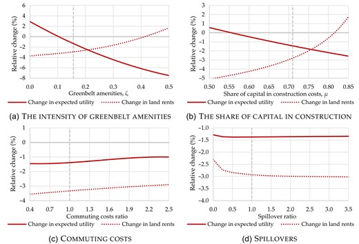
No Greenbelt Scenario for Different Parameter Values.
Notes: I estimate the effects using parameters estimated in column (6) of Table 5. The dashed lines indicate the baseline parameters. I consider the scenario where all greenbelts are removed. In (c), commuting cost parameters |$\lbrace \varkappa _\mathcal{rd}, \varkappa _\mathcal{rw}, \varkappa _\mathcal{oth}\rbrace$| are multiplied by the commuting cost ratio. In (d), I multiply spillover parameters |$\lbrace \hat{\psi }, \hat{\gamma }, \hat{\lambda } \rbrace$| with the spillover ratio.
Results of Counterfactual Analyses.
| Scenario 1: 10% reduction in greenbelts | Scenario 2: no greenbelts | Scenario 3: counterfactual greenbelts | |
|---|---|---|---|
| (1) | (2) | (3) | |
| Panel A: baseline | |||
| Change in expected utility (in %) | −0.250 | −1.400 | 0.332 |
| Change in overall land rents (in %) | 0.442 | −2.674 | 4.457 |
| Change in output (in %) | −0.172 | 1.017 | −1.100 |
| Change in average floor space price (in %) | −2.350 | −7.320 | 6.719 |
| Change in average wages net of commuting (in %) | −0.171 | −0.184 | −0.203 |
| Change in total developable land (in %) | 8.804 | 54.480 | −5.517 |
| Change in total floor space (in %) | 1.563 | 6.780 | −3.208 |
| Panel B: no greenbelt amenities, |$\zeta =0$| | |||
| Change in expected utility (in %) | 0.743 | 2.747 | −0.714 |
| Change in overall land rents (in %) | 4.060 | −0.318 | 7.370 |
| Change in output (in %) | 1.696 | 2.782 | 0.509 |
| Change in average floor space price (in %) | −1.619 | −6.618 | 7.408 |
| Change in average wages net of commuting (in %) | −0.060 | 0.036 | −0.115 |
| Change in total developable land (in %) | 8.804 | 54.480 | −5.517 |
| Change in total floor space (in %) | 2.952 | 8.054 | −2.197 |
Notes: I take the parameter values estimated in column (6) of Table 5.
Whether greenbelts increase welfare also depends critically on the value of μ. I find in Figure 2(b) positive utility effects of greenbelts for workers when μ exceeds 0.55. With a high μ, it is economical to build in higher densities in existing urban areas. Hence, the removal of greenbelts mostly leads to a loss in amenities, while the supply effect is limited. On the other hand, with a low μ, buildings are land intensive and the removal of greenbelts will mean that the reduction in floor space prices due to increased supply is more substantial. With respect to land rents, a high μ means that the benefits of land are larger because building construction is capital intensive. In sum, when μ is higher, it is easier to build taller, and therefore revenues per unit of land increase.
Figure 2(c) shows that the size of commuting costs does not have much of an influence on the aggregate welfare effects of greenbelts. I have studied the importance of spillovers in more detail in Figure 2(d). I then show the welfare effects of removing greenbelts for lower and higher parameters capturing spillovers |$\lbrace \hat{\psi }, \hat{\gamma }, \hat{\lambda } \rbrace$| than originally estimated. The welfare effects when greenbelts are removed for different values of spillovers are hardly affected by the size of the spillover parameters. Kline and Moretti (2014) showed that agglomeration economies are a localised market failure that, given their stylised model, cancels out in the aggregate when the agglomeration elasticity is constant across space. Hence, agglomeration economies and congestion do not exactly cancel out in my model, which explains why there is a tiny change in welfare if spillovers are absent.
All in all, whether greenbelts generate positive welfare effects depends predominantly on the interplay between the intensity of greenbelt amenities, |$\zeta$|, and how easy it is to build, μ. I observe that, with strong greenbelt amenities and a reasonably high share of capital in construction costs, greenbelts are welfare improving.
4.2.3. Counterfactual scenario 3
Let us now turn back to Table 6. The third counterfactual scenario describes what would happen if all major cities in England had greenbelts, which can be seen as a push towards more environmentally friendly urban planning. I explain the procedure to determine these so-called counterfactual greenbelts in Online Appendix D.2. I observe in Table 6 that the equivalent income change is approximately |$0.3\%$|, so the overall effect is small. Hence, it is unlikely that adding more greenbelt land will lead to substantial positive welfare effects. Total land revenues increase by approximately |$4.3\%$| because land becomes more scarce and therefore much more expensive. Housing affordability thus strongly reduces as prices rise by |$6.8\%$|.
I have explored the issue of increasing greenbelt land further by calculating utility and land rents for different scenarios. Using the counterfactual cities as shown in Online Appendix D.2, I consecutively increase the size of the greenbelt ‘doughnut’ around each city. Figure 3 shows that expected utility is monotonically increasing in the share of greenbelt land in England, although the utility gains are essentially flat beyond a share of greenbelt land that equals |$30\%$|. Land rents are also monotonically increasing in the total amount of greenbelt land. I caution, however, that, for very high shares of greenbelt land, non-linear effects not taken into account in the current model may become relevant. For example, accommodating all workers and residents in currently existing cities may become prohibitively expensive.
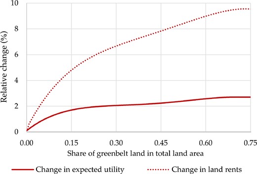
Increasing Greenbelt Land.
Notes: I estimate the effects using parameters estimated in column (6) of Table 5. Here, I calculate changes with respect to a situation where all greenbelts are removed.
In Online Appendix D.6, I provide a robustness analysis for these findings. First, I use the parameters identified when using all MSOAs (see column (1) of Table 5) or when using locations in 1973 greenbelts, which leads to similar results. Second, because one may be concerned about the identification strategies used to identify spillovers, I also estimate counterfactuals where I borrow parameters from the literature, leaving the results essentially unaffected.
4.3. Counterfactual Analyses and Welfare—Local Effects
Although aggregate effects may seem modest, local effects are large in relative terms. I plot the local effects of scenario 2 (no greenbelts) in Figure 4.
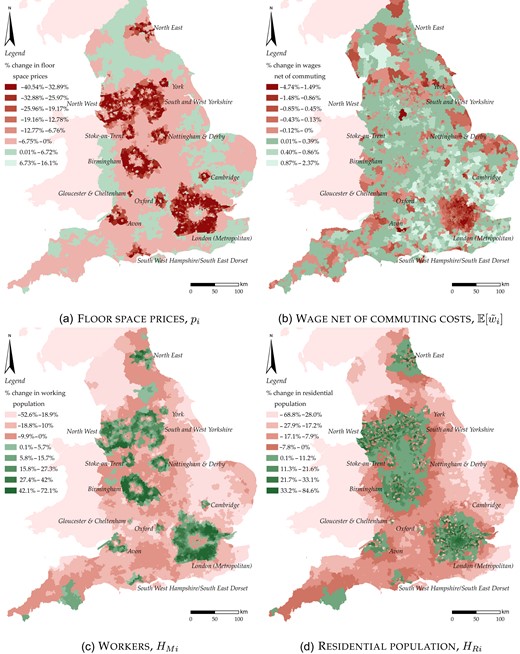
Counterfactual 2: No Greenbelts.
Notes: I estimate the effects using parameters estimated in column (6) of Table 5. I consider the scenario where all greenbelts are removed.
In some locations, floor space prices drop substantially (Figure 4(a)). In former greenbelt areas, this price drop can be as high as |$40\%$|. A key reason why prices drop in greenbelts is the loss in amenities. Outside greenbelts prices also drop substantially due to an increased supply of floor space. For example, in cities like London, Manchester and Birmingham, prices drop by 5%–|$20\%$|. Given that England’s cities are known to be expensive (Hilber and Vermeulen, 2016), removing greenbelt land seems to imply a substantial improvement in housing affordability. Wage effects are considerably smaller on average (see Figure 4(b)). Wages decrease in Greater London because of longer commutes, but the effects are small.
In Figure 4(c) I show that employment moves from city centres to former greenbelt areas. The relative increases in employment range from 5%–|$70\%$|. This may seem large, but note that these are relative differences. Because there were hardly any jobs in many former greenbelt areas in the first place, the relative increase in jobs is large. However, absolute changes are smaller. In Online Appendix D.3, it is shown that the absolute changes are relevant, but are too small to fundamentally change England’s urban structure.
For the residential population, the picture is somewhat similar (see Figure 4(d)). Because cities and their surrounding areas are now considerably cheaper, residents prefer to live in and around cities on former greenbelt land. At the same time, residents move into the inner cities of London and Birmingham. There are two reasons why people are doing this. First, given that production moves partly to former greenbelt areas, prices in city centres tend to be lower. This makes it attractive for people to move into city centres (which in turn increases floor space prices again). Second, areas close to former greenbelt areas lose greenbelt amenities, which in relative terms makes areas of central cities more attractive. One may be concerned that it is very unlikely that city centres will accommodate many new residents because other restrictions, such as height restrictions, floor-area restrictions and restrictions on new buildings in historic districts, may apply in central cities. However, when I plot the change in demand for floor space, it appears that the total amount of floor space is roughly constant in inner cities, so it is in actuality the space that lies empty due to firms moving to former greenbelt areas that is occupied by residents.
In Online Appendix D.6, I also consider the local effects of the other scenarios (i.e., the |$10\%$| reduction in greenbelts and the counterfactual greenbelts). The baseline mechanisms underlying the predictions discussed above hold up.
In Online Appendix D.6, I further calculate correlations between predicted percentage effects of specifications with different parameters. I show that the bivariate correlations with predicted local effects are mostly above 0.95; hence, the results are very similar. If I set amenities to zero, I find that correlations with the baseline counterfactual values are somewhat lower. This is not surprising given that greenbelt amenities play a pivotal role in explaining the local effects. Because of the fact that in the absence of greenbelt amenities, locations do not become less attractive when greenbelts are removed, I find that people move particularly to former greenbelt areas where there is a greater availability of cheap floor space. By contrast, the bivariate correlations with the predicted effects if I set spillovers to zero are very high, confirming that the main results can be explained mostly by the presence of greenbelt amenities and the share of capital in construction.
Interestingly, although commuting costs do not materially influence the aggregate effects, they are important for changes in the residential population. With low commuting costs, the effects of removing greenbelts are far more spread out, as residents can now commute long distances without incurring high costs. Given the current level of commuting costs, commuter towns like Milton Keynes, Reading and Ashford are all relatively far away.34 For lower commuting costs, commuter towns are more relevant, but become partly obsolete when removing greenbelts because residents do not have to ‘leapfrog’ greenbelts anymore. This, in turn, will considerably shorten commuting trips. With high commuting costs, the changes in residential population are much more contained to the areas that were formerly designated as greenbelt land.
5. Conclusions
In this paper, I have investigated the economic effects of greenbelt policy that prohibit new construction beyond a predefined boundary. I focus on England, where |$13\%$| of the land area is designated greenbelt land. Greenbelts were constituted between the 1950s and 1970s—a time when cities were much smaller—and have hardly changed ever since.
Using reduced-form regressions, I first establish that the restrictions implied by greenbelts are binding: within greenbelts the density is more than |$50\%$| lower. Greenbelts also imply positive amenity effects as measured by house prices. These effects are relatively local and are mostly relevant within 500 m. Still, given that approximately |$27\%$| of all dwellings in England lie within 500 m of greenbelt land, many properties are affected by greenbelt amenities.
I proceed by setting up a general equilibrium model that takes into account the effects of greenbelts on amenity values and housing supply. Moreover, I take into account commuting, mode choice, congestion on the road and agglomeration economies, all of which I show to be empirically relevant.
A counterfactual analysis then shows that greenbelt policy increases the utility of workers: when removing all greenbelts, the equivalent income decrease caused by greenbelts is roughly |$1.5\%$|, which amounts to £10 billion a year. On the other hand, monetary gains accrue to absentee landowners as total land revenues are around |$1.3\%$| higher. This amounts to £650 million per year. When greenbelts are removed, property prices inside greenbelts drop by |$20\%$| or more, but outside greenbelts prices also drop substantially due to an increased supply of floor space. For example, in cities like London, Manchester and Birmingham, prices drop by approximately 5%–|$20\%$|. Given that England’s cities are known to be expensive, removing greenbelt land seems to imply a substantial improvement in housing affordability.
Hence, greenbelts seem to imply overall welfare gains, but inevitably they worsen housing affordability. The finding of positive welfare effects critically depends on the strength of greenbelt amenities, which may depend on the local context (such as the quality of provided open space and cultural traits). Only when greenbelt amenities are strong enough, greenbelts imply benefits to residents. Interestingly, agglomeration economies do not seem to play an important role, which is in line with Kline and Moretti (2014), who argued that agglomeration economies are a localised market failure that cancels out in the aggregate.
Additional Supporting Information may be found in the online version of this article:
Online Appendix
Replication Package
Notes
The data and codes for this paper are available on the Journal repository. They were checked for their ability to reproduce the results presented in the paper. The replication package for this paper is available at the following address: https://doi.org/10.5281/zenodo.8260847.
This paper has received the Sakıp Sabancı International Research Award 2020. Mohammad Saeed Zabihidan provided useful research assistance in the early stages of this project. Paul Cheshire and Jos van Ommeren are thanked for their particularly helpful discussions. I also thank the editor, Barbara Petrongolo, four anonymous referees, Gabriel Ahlfeldt, Federico Curci, Robert Elliott, Sofia Franco, Steve Gibbons, Stephan Heblich, Christian Hilber, Matthias Kalkuhl, Joris Klingen, Camille Landais, Michael Pflüger, Tobias Seidel, Saeed Tajrishy, Matthew Turner, Erik Verhoef, Xiao Yu, as well as seminar participants in Birmingham, Düsseldorf, London, Lugano, Madrid, Neuchâtel, Potsdam, Philadelphia, St. Petersburg, Vancouver and Würzburg for their useful input. Data on historic transportation networks were kindly provided by Miquel-Àngel Garcia-López, Ilias Pasidis and Elisabet Viladecans-Marsal.
Footnotes
When using calibration, parameters are chosen based on other studies and research contexts. By contrast, when estimating parameters, current data are used and empirical strategies are devised to obtain the model’s parameters.
An older paper by Cheshire and Sheppard (2002) attempts to evaluate the welfare effects of land-use regulation for the city of Reading by relying on a monocentric city model. They found that expanding the city will yield positive welfare effects. However, the model is subject to several strong functional form assumptions and does not include commuting, congestion and agglomeration economies.
Turner et al. (2014), meanwhile, did not present a general equilibrium analysis of supply restrictions, because they focused on the effects of areas close to municipal borders. By contrast, I focus on a situation where land-use regulation is ubiquitous and where general equilibrium effects are expected to be sizeable.
Greater London was the first urban area to discuss the implementation of a greenbelt and did so before World War II. However, it was only in the late 1950s that greenbelt land around London was officially approved. The greenbelt area increased five-fold in 1965, while in 1971, the government decided to extend the Metropolitan Green Belt to include almost all of Hertfordshire. The Bristol and Bath Green Belt was adopted locally in 1957 and approved in 1966. The North-West greenbelt around Manchester, Liverpool and Leeds was first considered in the early 1960s, but it was approximately 20 yr before it received official approval. The same holds for the greenbelt around York, which was formally created in 1980 after decades of being a local policy.
For example, the total hectares of greenbelt land in 1997 was 1,652,310, while it was 1,638,610 in 2013, a change of less than |$1\%$|, which may as well be due to measurement error.
In the empirical analysis, I will therefore include specifications where I distinguish between different types of greenbelt land.
Specifically, I first match a sale to an EPC using the primary address object name, secondary address object name, street name and postcode. I then keep the certificate that is closest in days to the sale. I repeat this exercise for unmatched properties, but allow the address identifiers to be different. The final round of matching matches on the full postcode.
The matching is more challenging for flats that often share an address, implying that the proportion of flats is reduced from |$23\%$| in the Land Registry sample to 3% in the final sample. My analysis therefore mainly focuses on single-family homes. One may be concerned that this implies sample selection bias. However, if I calculate floor space prices at the MSOA prices using the full Land Registry dataset and using the matched dataset, the correlation is 0.988. Moreover, I show in Online Appendix B.2.7 that the results are essentially the same if I only include apartments.
More specifically, I drop transactions with prices that are above £1.5 million or below £15,000 and properties that are smaller than 25 m2 or larger than 250 m2. Together this applies to less than |$0.5\%$| of the data.
To ensure that measurement error in greenbelt land does not bias my results, I also estimate regressions where I only include observations from the closest census year 2011, which does not change the results (see Online Appendix B.2.7 for more details).
The results of this regression are available upon request. Housing characteristics included in the regression are the log of house size, house type (i.e., terraced, semi-detached or detached), a dummy indicating whether the house is newly built, the number of rooms, the number of habitable rooms, the floor level (if it is an apartment), the height of the average floors, the number of floors of the building, whether the property has a fireplace and the quality of the windows, the roof, walls and overall energy efficiency. I also include a dummy indicating whether the property is freehold. All the coefficients have the expected signs and magnitudes.
The average speed on motorways is obtained from statista.com.
One may argue that I underestimate the speed of intercity services, say, between London and Birmingham. However, for most commutes, only local trains are used that have lower average speeds.
Postcodes are on average 10 ha due to a few very large postcodes.
The highest floor space can be found in London in the borough of Kensington-Chelsea.
The more convincing identification strategies (columns (3)–(6)) show larger supply effects. In these specifications, I use a control group of areas that are similar and geographically close. The effect is thus stronger because I compare areas that are only part of cities or towns to areas that are restricted by greenbelts. This helps to identify arguably the ‘true’ supply effect of greenbelts.
I also consider including observations on either side of the border, as in columns (6) and (7) of Table 3. However, coefficients are then too imprecise to yield much information.
Other than heterogeneity through idiosyncratic preferences, I abstract from heterogeneity in, e.g., income, such as in Tsivanidis (2020) or Gaigné et al. (2021). Unfortunately, I lack good micro-data on incomes. Moreover, allowing for heterogeneous workers would render the model much more difficult and probably obscure the key forces at work.
One may argue that commuting costs contain a time and pecuniary component. I do not dispute this, but allowing for this type of commuting cost goes beyond the scope of this paper. Importantly, given the value of time obtained in empirical studies (see Small and Verhoef, 2007), it appears that time costs far exceed the pecuniary component of commuting costs.
I may also allow for the decay of residential density, as in Ahlfeldt et al. (2015). In the current paper, it appears that this decay parameter is difficult to estimate but is, if anything, very high. In other words, density effects only pertain to one’s own MSOA, which is in line with the strong decay found in Ahlfeldt et al. (2015).
More specifically, I choose |$\varsigma$| in such a way that |$(\sum _{j=1}^\mathcal {L} \sum _{m=1}^3 F_{Mjm})/ (\sum _{j=1}^\mathcal {L} \sum _{m=1}^3 F_{Rjm})$| is equal to the overall ratio of commercial floor space to residential floor space in the data. Workers need relatively less office space than residential space, so |$\varsigma \lt 1$|.
The optimal use of floor space is given by |$F_{jm}^{*} = ((1-\alpha ) Y_{jm})/p_j$|, while the optimal use of labour is |$H_{jm}^{*} = (\alpha Y_{jm})/\varsigma w_j$|. I then substitute |$F_{jm}^{*}$| and |$H_{jm}^{*}$| into |$Y_j$| to obtain |$\Omega _j$|. As in Ahlfeldt et al. (2015), |$\Omega _{j}$| is identified up to a normalisation constant. I normalise |$\bar{\upsilon }_{j,\mathcal{rd}}=1$|, while I choose values of |$\bar{\upsilon }_{j,\mathcal{rw}}$| and |$\bar{\upsilon }_{j,\mathcal{oth}}$| to ensure that |$\Omega _{j}=\Omega _{j,\mathcal{rd}}=\Omega _{j,\mathcal{rw}}=\Omega _{j,\mathcal{oth}}$|.
In a previous version of this paper, I also allowed for the direct effects of greenbelts on productivity. I did not find clear evidence for a ‘productive amenity’ effect of greenbelts. More importantly, the results of the counterfactuals are hardly affected by the inclusion of direct effects of greenbelts, while they complicate the estimation. These results are therefore available upon request.
I show in Online Appendix C.4 that congestion at the residential location indeed matters less.
Note that |$\varsigma$| does not capture the share of commercial space to total real estate space, but it is a parameter that ensures that the ratio of commercial floor space to residential floor space matches the data. In 2008, the total commercial and industrial space was 562 million m2, while the total residential floor space was 22.2 million dwellings |$\times$| 92 m2|$=2.042$| billion m2. Hence, the ratio of commercial to residential floor space was 0.2745. In the baseline scenario, the total amount of commercial floor space predicted by the model is 1,543, while the predicted amount of residential floor space is 805. Hence, to adjust the amount of commercial floor space to match the ratio to residential floor space, I set |$\varsigma =0.1435$|.
To be more specific, I exclude only |$1\%$| of commuters by road, |$1.1\%$| of commuters by rail and |$1.2\%$| of commuters by other modes.
I obtain data on estimated household incomes using MSOA by the Office of National Statistics from 2011.
There are nine government regions in England. When intersecting those with 12 greenbelts, I end up with 32 areas.
More specifically, for each location i, I calculate the travel time to all j. I then generate variables that sum workers for a given travel time ring, implying that I will include 60 variables; the total number of workers between 0–2-minute travelling, 2–4-minute travelling, etc.
I show in Online Appendix C.4 that my results are robust to omitting home location fixed effects.
If I fit the exponential decay function through Rosenthal and Strange’s preferred estimates, I obtain decay parameters ranging from 0.027–0.064.
I obtain data on estimated land prices for 326 local authorities from the Department for Communities and Local Government from 2014. I deflate land prices to 2011 values using the consumer price index. The estimated total land revenues at i are then given by |$p_i F_i - r K_i$|.
Of course, greenbelt policy is an important example of a supply constraint, but it is definitely not the only one.
For example, to travel from Milton Keynes, Reading and Ashford to the City of London takes, 54, 56 and 63 min, respectively.
