


Abstract
Based on artefactual field experiments, we investigate whether finance professionals differ from a sample of the working population in terms of industry-relevant preferences and personality traits. When adjusting for socioeconomic characteristics, we find only few and less marked differences: finance professionals are less risk averse, less trustworthy, show higher levels of psychopathy and are more competitive than participants from the general population. In an additional survey, experts with hiring experience consider industry selection, self-selection and imprinting by industry norms as explanatory for the observed subject pool differences.
The finance industry is one of the biggest industries worldwide1 and bears systemic relevance and risk for the economy in general (Acharya et al., 2016). It is characterised by peculiar features: Financial products are typically complex (Brunnermeier and Oehmke, 2009; Inderst and Ottaviani, 2012a) and information asymmetries as well as conflicts of interest exist in financial markets (Cain et al., 2005; Inderst and Ottaviani, 2012b). This context makes room for severe problems, which can be aggravated by the fact that inferior decisions and advice by professionals are difficult to detect even ex post (Bluethgen et al., 2008) and, consequently, hard to monitor and prevent (Egan et al., 2019). In such an environment, the main protagonists—finance professionals—shape the finance industry with their personality traits and economic preferences, such as their altruism, risk tolerance, honesty and trustworthiness. These traits and preferences can be expected to determine professionals’ behaviour, which has direct consequences for both their clients and society as a whole. Thus, it is important to understand what kind of people work in the finance industry—even more so, given that the public perception has not been overall positive. As a consequence of the financial crisis of 2008 and subsequent scandals, such as the Libor manipulation, the public reputation of finance professionals took a nose dive. Many times the resulting public debate and negative press coverage have drawn an undifferentiated picture of finance professionals as being greedy and dishonest and substantially different from other occupational groups.2
In the previous literature, most studies on finance professionals’ behaviour only focus on one particular behavioural bias or a single economic preference dimension.3 Moreover, several previous studies on behavioural differences between finance professionals and other populations do not account for individual-level characteristics (see, e.g., Glaser et al., 2005; Haigh and List, 2005 and Kaustia et al., 2008), although economic preferences and behavioural traits have been shown to correlate with sociodemographic factors (see, e.g., Falk et al., 2018). With our study, we shed light on the economic preferences and personal characteristics of finance professionals by comparing a selection of industry-relevant economic preferences and personality traits between a sample of finance professionals and a randomly selected sample of the general working population (henceforth also referred to as the ‘general population’). We contribute to the literature by providing a comprehensive picture of a multitude of characteristics to gain insights along which dimensions finance professionals differ from people employed in other industries.
In particular, we conducted a pre-registered artefactual field experiment, eliciting participants’ risk preferences, distributional preferences, trustworthiness, dishonesty and various personality traits. In total, 298 financial analysts,4 investment advisers,5 traders, fund managers and financial brokers, and 395 participants from a randomly selected sample of the Swedish working population—excluding finance professionals—participated in our study. Note that our sample of finance professionals is not representative for all people working in the finance industry, which would be an exceedingly heterogeneous group (Huber and König-Kersting, 2022). Rather, we deliberately chose the subset described above, as these people are at the core of financial decision-making or central for customers in the way they manage portfolios, provide analyses and manage funds.
A multi-faceted line of research has established that preference relations and personal traits tend to be systematically correlated with various demographic and socioeconomic characteristics (see, e.g., Croson and Gneezy, 2009; Algan and Cahuc, 2010; Niederle and Vesterlund, 2011 and Falk et al., 2018). Considering that the groups of finance professionals and the general working population are likely to differ systematically in socioeconomic characteristics (e.g., due to self-selection into the industry or the selection of the industry itself), not adjusting for this potential source of heterogeneity may induce an omitted variable bias in estimating effects between subject pools: differences in preferences and traits may be spuriously attributed to the variation in a subject pool indicator, although (part of) the variation may actually be due to systematic heterogeneity in socioeconomic characteristics. By adjusting the differences between subject pools for the variability in potentially relevant socioeconomic drivers (obtained from Statistiska centralbyrån (SCB; Statistics Sweden)), we can infer whether differences between the subject pools actually persist over and beyond the variation explained by participants’ socioeconomic background.
In order to examine preferences and personality traits that are relevant for financial decision-making, our experiment involved four incentivised tasks. In particular, we set up single choice lists (Eckel and Grossman, 2002) to assess participants’ attitudes toward risk, losses and skewness, and elicited distributional preferences (Kerschbamer, 2015), trustworthiness (Berg et al., 1995) and cheating behaviour (Fischbacher and Föllmi-Heusi, 2013). In addition, we analyse individuals’ personality traits, measured by means of the Big-Five personality test by Rammstedt and Oliver (2007), the Dark Triad inventory by Jonason and Webster (2010) and the sub-module of the Work and Family Orientation questionnaire focusing on competitiveness (Helmreich and Spence, 1978).
We find that the sample of finance professionals, as compared to participants from the general population, is significantly more risk tolerant, more selfish, less trustworthy, more competitive and shows higher levels of narcissism, psychopathy and Machiavellianism. These results suggest that finance professionals effectively differ from people employed in other industries—particularly in those characteristics that the general public is keen to pick up to sketch the dark side of the finance industry. This finding is in line with the assumption that the finance industry—in our case proxied by financial analysts, investment advisers, traders, fund managers and financial brokers—is indeed different to other industries. However, this argument leaves aside that finance professionals also differ from the general working population along several socioeconomic dimensions.
A substantial part of the differences between finance professionals and the general population can actually be explained by the variation in participants’ socioeconomic characteristics. We observe that after adjusting the differences between subject pools for gender, age, income and educational background, finance professionals tend to be only slightly more risk tolerant, remain less trustworthy, show a slightly increased level of psychopathy and are still more competitive than comparable participants from other industries. While several differences entirely disappear when adjusting for sociodemographic characteristics, the effect sizes of those characteristics that remain statistically significant tend to be deflated. Thus, given the number of preferences and traits examined in our study, our results indicate that finance professionals and people employed in other industries with comparable socioeconomic background are not that different after all.
Finally, we shed light on potential drivers (channels) of subject pool differences by running a pre-registered expert survey. We recruited 205 experts from within the finance industry with hiring experience (i.e., human resource specialists and middle managers) to investigate whether they consider any of the three channels—industry selection, self-selection or imprinting by industry norms—explanatory for behavioural patterns of the four experimental tasks showing significant subject pool differences (i.e., attitudes toward risk, trustworthiness, competitiveness and psychopathy). We find that all three channels are considered to play at least some role for risk aversion, trustworthiness and competitiveness. For psychopathy, only self-selection into the industry is perceived somewhat explanatory for subject pool differences. These findings indicate that experts do not conceive self-selection, industry selection and imprintment to be mutually exclusive concepts. The survey results are consistent with the assumption that the three channels are mutually correlated, presumably in a self-reinforcing manner.
1. Experimental Procedure
We conducted an online experiment in Sweden in cooperation with Statistics Sweden (SCB), who invited participants and provided a set of predefined variables from the registry for those participants who completed the experiment.6 The hard-copy invitations were distributed to a subset of highly skilled finance professionals (FP) and a random sample of Sweden’s general working population (GP ; excluding finance professionals). In particular, invitations were sent out to all (but only) finance professionals with SCB’s job code classifications ‘2413’ (financial analysts and advisers), ‘2414’ (traders and fund managers) and ‘3311’ (financial brokers). While the average ages of both subject pools are almost identical (FP = 41.0, GP = 41.2), the fraction of females (FP = 24.5%, GP = 41.0%), the annual gross income (in Swedish Krona, SEK) (FP = 711,268, GP = 396,878) and the fraction of participants without a university degree (FP = 8.1%, GP = 28.1%) differ significantly (|$p \lt 0.001$| for all three comparisons) between the two samples and reveal first industry-specific peculiarities of the finance sector. Further details and additional information on the recruitment, data collection and experimental implementation are provided in Online Appendix A, where we report and discuss response rate analyses and self-selection effects.7
Once participants logged in to the software (programmed in oTree; Chen et al., 2016) using a personal identifier, they were presented with a detailed outline of the experiment and could continue once they provided informed consent. The experiment consisted of four parts that were presented to each participant in random order. The tasks on attitudes toward risk, losses and skewness, the distributional preferences elicitation, the trust game and the cheating task were incentivised, as is common practice in experimental economics. The surveys on personality traits (i.e., the Big-Five and Dark Triad inventories, as well as the sub-scale of the Work and Family Orientation questionnaire on competitiveness) were unincentivised, as, again, is standard in the literature. At the end of the experiment, one of the incentivised measures was randomly selected for payout. Details of the experimental tasks, treatment variations and payments are described in Section 2. For completing the online experiment, participants received a participation fee of 100 Swedish krona (SEK ).8 The experimental data were collected between January 7 and February 24, 2019. In total, 298 finance professionals and 395 people from the general population, working in other sectors, completed the experiment. The experiment was conducted in Swedish and took on average 15 minutes to complete. The average payment to participants was 211.13 SEK (SD |$= 51.92$|), which was approximately $23.50 by the time the experiment ended.9 To ensure full privacy of the data collected during the experiment, payouts were handled by the third-party survey firm Enkätfabriken.
In addition to the data collected in the online experiment, we obtained register data from SCB for each participant who completed the experiment. In the analysis of the experimental results, we use part of the registry data as adjustment variables, in particular, participants’ gender (binary indicator for female), age (in years), net income from major employment in 2017 (in thousand SEK) and maximum education level (dichotomous indicators for high school education or less, university education less than or equal to three years and university education greater than three years).10
A detailed summary of participants demographics compared to the characteristics of the sample invited is presented in Table A1 in Online Appendix A. In particular, Table A1 reports the number of respondents and non-respondents per category of several sociodemographic characteristics, separated for both samples, as reported by SCB. Moreover, we report |$\chi ^2$| tests comparing whether participants in our samples differ significantly from those who have been invited by SCB, but did not participate in the experiment. We report self-selection effects into the experiment in terms of gender, age, country of birth, income and education for the general population sample, and self-selection effects with respect to gender, age and education for the finance professional sample.
2. Experiments and Results
We address each of the five parts in our experiment separately. In particular, each subsection briefly motivates our research agenda, provides a concise description of the experimental implementation, relates our contribution to the previous literature and discusses the main findings related to the particular part of our study. Each of the subsections is accompanied by a separate annex (see Online Appendices B–E), providing additional details on the experimental design and the definition of measures, descriptive results, as well as supporting and ancillary analyses.
The figures in the main text show the coefficient estimates of the dummy variable indicating the finance professional subject pool in the corresponding regression models (which are presented in the accompanying tables in the appendices).
For the sake of interpretability, we report standardised effect sizes whenever suitable. We follow the Open Science Collaboration (2015) and Camerer et al. (2018) and determine standardised correlation coefficients (|$r_s$|) and 95% confidence intervals (CIs) for key effects relevant to our research questions—in particular, the effects attributable to differences between the two subject pools.11 Standardised correlation coefficients allow us to provide a unified measure of the magnitude of an effect, which is independent of the scaling of the dependent variable and the statistical method used to determine the effect. As a rule of thumb, we follow the guidelines proposed by Cohen (1992) and refer to correlation coefficients with thresholds of 0.1, 0.3 and 0.5 as being indicative of small, medium and large effects, respectively.
In an exploratory analysis, we examine whether the various preferences and characteristics differ systematically between the three different job functions from which finance professionals were sampled; the results are tabulated and discussed in Online Appendix F. An additional exploratory analysis presents correlations between the different preferences and personality traits for the two subject pools in Table G1 in Online Appendix G. In general, we find qualitatively homogeneous correlational patterns within both samples.
2.1. Attitudes toward Risk, Loss and Skewness
Since risk-taking is at the core of financial decision-making (Nosić and Weber, 2010; Weber et al., 2013), the question of whether finance professionals differ in their risk preferences from other populations arises naturally. The qualification for the finance profession might require a certain attitude toward risk, and the individual risk appetite might change with specific training and day-to-day experience in making risky decisions. Despite the regular exposure to risky decision environments, there is some evidence of higher myopic loss aversion (Haigh and List, 2005) and a more intuitive risky decision-making process (Gilad and Kliger, 2008) among finance professionals as compared to student participants. Moreover, existing evidence indicates that professionals’ behaviour can be explained by prospect theory (Gurevich et al., 2009; Abdellaoui et al., 2013), and that professionals—similar to laypeople—perceive risk as the likelihood of incurring losses rather than symmetric deviations from the expected return (Holzmeister et al., 2020). Since a mere focus on ‘risk as variance’ might fall short of contributing to a better understanding of finance professionals’ behaviour in ‘risky’ decision environments, we address attitudes toward a broad spectrum of characteristics that are intimately related to the concept of risk. We ask the following research question: is there a difference in tolerance toward volatility, skewness and losses between finance professionals and people from the general working population?
2.1.1. Method
To answer this research question, we implemented a series of four single choice lists, based on Eckel and Grossman (2002). In particular, we varied the lotteries’ prospective payoffs in such a way that a single characteristic of the gambles was systematically varied while holding the other characteristics constant. In each of these four tasks, participants were presented with a menu of six lotteries, and were asked to indicate which of the prospects they prefer. In all four tasks, the lotteries were decreasing in their risk-adjusted expected return. To assess participants’ attitudes toward risk, skewness and losses, we varied two characteristics of the gambles—the skewness of lottery outcomes and the possibility to incur losses—using a factorial design.
For the sake of denotation, we introduce the indicator functions |$S_i$| and |$L_i$| for skewness and losses, respectively. The parametrisation of the four tasks is shown in Table 1. While the lottery outcomes in tasks |$S_0L_\times $| were symmetric, the outcomes were positively skewed in tasks |$S_1L_\times $| (without altering their SD). In tasks |$S_\times L_0$|, the minimum outcome was strictly positive, whereas a constant was subtracted from all payoffs in tasks |$S_\times L_1$| (i.e., the prospects’ SD and skewness were unaffected). While a participant’s lottery choice in |$S_0L_0$|, which only involves symmetric gambles in the non-negative domain, serves as a proxy of the decision-maker’s risk tolerance, the other preference types are characterised by the difference in the lottery choices between tasks. For instance, |$S_0L_1 - S_0L_0$| captures the difference in choice behaviour between tasks |$S_0L_1$| and |$S_0L_0$| that is attributable to loss tolerance; likewise, |$S_1L_0 - S_0 L_0$| accounts for the difference in choice behaviour attributable to attitudes toward skewness.12 Further details regarding the implementation, as well as descriptive and supplementary results are provided in Online Appendix B.
Parametrisation of the Four Tasks Used to Elicit Participants’ Attitudes Toward Risk, Losses and Skewness.
| Task |$\boldsymbol {S_0L_0}$| | |||||
|---|---|---|---|---|---|
| |$x_1$| | |$x_2$| | ||||
| 50% | 50% | EV | SD | SK | |
| 96.0 | 96.0 | 96.0 | 0.0 | ||
| 80.0 | 128.0 | 104.0 | 24.0 | 0.0 | |
| 64.0 | 160.0 | 112.0 | 48.0 | 0.0 | |
| 48.0 | 192.0 | 120.0 | 72.0 | 0.0 | |
| 32.0 | 224.0 | 128.0 | 96.0 | 0.0 | |
| 16.0 | 240.0 | 128.0 | 112.0 | 0.0 | |
| Task |$\boldsymbol {S_0L_1}$| | |||||
| x1 | x2 | ||||
| 50% | 50% | EV | SD | SK | |
| 16.0 | 16.0 | 16.0 | 0.0 | ||
| 0.0 | 48.0 | 24.0 | 24.0 | 0.0 | |
| −16.0 | 80.0 | 32.0 | 48.0 | 0.0 | |
| −32.0 | 112.0 | 40.0 | 72.0 | 0.0 | |
| −48.0 | 144.0 | 48.0 | 96.0 | 0.0 | |
| −64.0 | 160.0 | 48.0 | 112.0 | 0.0 | |
| Task |$\boldsymbol {S_1L_0}$| | |||||
| x1 | x2 | x3 | |||
| 50% | 49% | 1% | EV | SD | SK |
| 96.0 | 96.0 | 96.0 | 96.0 | 0.0 | |
| 82.1 | 123.9 | 223.0 | 104.0 | 24.0 | 1.1 |
| 68.2 | 151.8 | 350.1 | 112.0 | 48.0 | 1.1 |
| 54.2 | 179.8 | 477.1 | 120.0 | 72.0 | 1.1 |
| 40.3 | 207.7 | 604.2 | 128.0 | 96.0 | 1.1 |
| 26.4 | 220.4 | 684.0 | 128.0 | 111.5 | 1.1 |
| Task |$\boldsymbol {S_1L_1}$| | |||||
| x1 | x2 | x3 | |||
| 50% | 49% | 1% | EV | SD | SK |
| 16.0 | 16.0 | 16.0 | 16.0 | 0.0 | |
| 2.1 | 43.9 | 143.0 | 24.0 | 24.0 | 1.1 |
| −11.8 | 71.8 | 270.1 | 32.0 | 48.0 | 1.1 |
| −25.8 | 99.8 | 397.1 | 40.0 | 72.0 | 1.1 |
| −39.7 | 127.7 | 524.2 | 48.0 | 96.0 | 1.1 |
| −53.6 | 140.4 | 604.0 | 48.0 | 111.5 | 1.1 |
Notes: Here Si and Li are indicator functions for skewness and losses, respectively; e.g., S1L0 indicates the task with skewed lottery outcomes in the gain domain. We indicate by x1, x2 and x3 the potential lottery outcomes in SEK. By EV, SD and SK we denote the lotteries’ expected value, standard deviation and skewness, respectively.
2.1.2. Results
Panel (a) of Figure 1 depicts the cumulative distributions of choices attributed to risk, skewness and loss tolerance, separated for finance professionals and the general population, respectively. While we report that finance professionals, on average, are significantly more risk tolerant than participants from the general population, we do not find evidence of systematic differences between the two samples with respect to attitudes toward skewness or losses (see the test statistics of Kolmogorov-Smirnov (KS) tests in panel (a) of Figure 1).
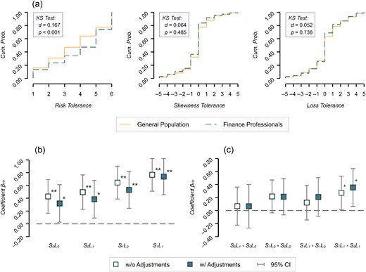
(a) Cumulative Distributions of Risk Tolerance (|$S_0L_0$|), Skewness Tolerance (|$S_1L_0 - S_0L_0$|) and Loss Tolerance (|$S_0L_1 - S_0L_0$|), Separated for the General Population and Finance Professional Samples. (b) Coefficient Plots for the Dichotomous Variable Indicating the Finance Professional Subject Pool in Ordinary Least-Squares Regressions for Each of the Four Tasks Eliciting Attitudes Toward Risk, Skewness and Losses. (c) Differences between Coefficient Estimates per Task, i.e., Estimates Isolating the Effects of Attitudes Toward Losses and Toward Skewness, Respectively. For Instance, |$S_0L_1 - S_0L_0$| Denotes the Difference in Choice Behaviour Attributable to Loss Tolerance (in Lotteries without Skewed Outcomes).
Notes: In (a) Kolmogorov-Smirnov tests are reported in boxes. Here |$n_{{{\it GP}}} = 395, n_{\it FP} = 298$|. In (b) and (c) |$S_i$|and |$L_i$| are indicator functions for skewness and losses, respectively; e.g., |$S_1L_0$| indicates the task with skewed lottery outcomes in the gain domain. Hollow markers show estimates from models without adjustments (n = 693); solid markers show estimates from models with adjustment variables (n = 688). Error bars indicate 95% confidence intervals based on robust standard errors. The regression estimates are summarised in Table B2 in Online Appendix B. |$^*\, p \lt 0.05,\ ^{**}\, p \lt 0.005.$|
Turning to panels (b) and (c) of Figure 1, these effects can be examined in more detail: panel (b) shows the differences in the average lottery choices between the finance professional and general population samples for each of the four tasks eliciting attitudes toward risk, skewness and losses. The coefficients represent the dichotomous variable indicating differences between the finance professional subject pool and the general population estimated using ordinary least-squares regressions summarised in Table B2 in Online Appendix B.
We find that the coefficient estimates of the dummy variable indicating the finance professional sample turns out being significantly positive in each of the four tasks, in both models not including and models including adjustment variables. While the significant coefficient for task |$S_0L_0$| immediately points toward a systematic difference in risk preferences (in the absence of skewness and losses), the coefficients for tasks |$S_0L_1$|, |$S_1L_0$| and |$S_1L_1$| only indicate that finance professionals, on average, are also systematically more willing to take risk in decision environments that involve skewed payouts and/or potential losses.
To isolate differences in choice behaviour attributable to skewness and loss tolerance between the subject pools, we illustrate the effect of the subject pool indicator variable on the differences in risky choices between tasks in panel (c) (see also the full regression results in panel (b) in Table B2 in Online Appendix B). In contrast to contributions by Haigh and List (2005) and Abdellaoui et al. (2013), we do not find evidence for systematic differences in participants’ loss tolerance between subject pools, neither in decision environments without skewed outcomes (|$S_0L_1 - S_0L_0$|) nor in decision environments with skewed outcomes (|$S_1L_1 - S_1L_0$|).13 Likewise, we do not find evidence for differences in skewness tolerance between subject pools if the lottery payoffs are non-negative (|$S_1L_0 - S_0L_0$|). If the decision situation involves the possibility to incur losses, however, our data suggest that finance professionals are more skewness tolerant than laypeople, but the effect size is small (|$r_s = 0.079$|, |$\rm{95\% CI} = [0.005, 0.155]$|).
Thus, we can conclude that finance professionals, on average, tend to be systematically less risk averse. While the difference in risk-taking behaviour between finance professionals and laypeople is in line with results reported in the literature (see, e.g., Kirchler et al., 2018; 2020 and Stefan et al., 2022), it should be noted that the magnitude of the effect is rather small in our sample (|$r_s = 0.120$|, |$\rm{95\% CI} = [0.046, 0.198]$|).
2.2. Distributional Preferences
For a long time, economic theory has assumed that economic decisions are only determined by the decision-maker’s self-interest. The study of ‘social preferences’ has become a focal point for a modified view on economic decision-making (see, e.g., Becker, 1974 and Rabin, 1993). With regards to the finance industry, there seems to be a common perception of finance professionals being closer to the conceptualisation of fully rational and selfish decision-makers. Yet, this view is not always supported by existing evidence on behavioural biases, for instance with regards to overconfidence (Deaves et al., 2010; Pikulina et al., 2017), anchoring (Kaustia et al., 2008) or framing (Roszkowski and Snelbecker, 1990). Moreover, existing experimental evidence suggests that distributional preferences are heterogeneous for various groups within a society (see, e.g., Fisman et al., 2015; 2017), and that economics students value efficiency more than equality compared to students in other fields and non-academics (Fehr et al., 2006). Since finance professionals have been trained in economic thinking, these findings might suggest that they are likely to differ from the rest of society in terms of distributional preferences. Furthermore, since finance professionals frequently act as ‘money doctors’ (Gennaioli et al., 2015)—involving decisions about other people’s money—distributional preferences can be of utmost importance. For instance, conflicts of interest in financial advice might be mediated by benevolent preferences toward the client, or rather be aggravated by purely selfish preferences (see, e.g., Angelova and Regner, 2013). Thus, we address the following yet unexplored research question: is there a difference in distributional preferences between finance professionals and people from the general population?
2.2.1. Method
We elicit distributional preferences using the equality equivalence test (EET ) introduced by Kerschbamer (2015). The EET consists of two lists with five binary choices each—one in the domain of disadvantageous inequality (x list) and one in the domain of advantageous inequality (y list). In both lists, each outcome of the five binary choices specifies a payoff for both the decision-maker and a randomly matched counterpart, and participants are asked to indicate whether they prefer option ‘Left’ or option ‘Right’. For all items in both lists, option ‘Right’ implies an equal payoff distribution, yielding 100 SEK for both participants. Outcomes associated with the option ‘Left’ in the x list increase from 60 to 140 SEK (in steps of 20 SEK) for the decision-maker, whereas the matched counterpart receives a payment of 160 SEK (disadvantageous inequality). The five prospectus outcomes for the decision-maker in the y list increase from 60 to 140 SEK, but the counterpart receives a payment of 40 SEK instead (advantageous inequality). Based on a participant’s switching points in the menu of binary choices in the two lists, the EET assigns one of nine archetypes of distributional preferences and a two-dimensional index of preference intensity, measured as the decision-makers’ willingness to pay in case the second player is ahead or behind, respectively. The parametrisation used in the experiment is summarised in Table 2.
Parametrisation of the Equality Equivalence Test.
| ‘Left’ | ‘Right’ | ||
|---|---|---|---|
| m | o | m | o |
| |$\boldsymbol {x}$| list | |||
| 60 | 160 | 100 | 100 |
| 80 | 160 | 100 | 100 |
| 100 | 160 | 100 | 100 |
| 120 | 160 | 100 | 100 |
| 140 | 160 | 100 | 100 |
| |$\boldsymbol {y}$| list | |||
| 60 | 40 | 100 | 100 |
| 80 | 40 | 100 | 100 |
| 100 | 40 | 100 | 100 |
| 120 | 40 | 100 | 100 |
| 140 | 40 | 100 | 100 |
Notes: The table shows the monetary payoffs (in SEK) for the ‘active’ player (m, for ‘me’) and the ‘inactive’ player (o, for ‘other’) for the two choices ‘Left’ and ‘Right’ for both the x list (disadvantageous inequality) and the y list (advantageous inequality).
2.2.2. Results
Panel (a) of Figure 2 shows the fractions of distributional preference types based on the EET, separated for the general population and finance professional samples. We find that the share of participants whose behaviour can be characterised as selfish is higher among finance professionals as compared to the general population (FP = 36.6%, GP = 26.8%; |$r_s = 0.104$|, |$\rm{95\% CI} = [0.030, 0.181]$|; |$p = 0.006$|), and that the proportion of inequality averse types is lower among finance professionals (FP = 10.1%, GP = 17.5%; |$r_s = 0.105$|, |$\rm{95\% CI} = [0.030, 0.182]$|; |$p = 0.006$|). We do not find evidence for systematic differences in the share of maximin (FP = 30.9%, GP = 27.6%; |$r_s = 0.036$|, |$\rm{95\% CI} = [-0.039, 0.111]$|; |$p = 0.347$|) and purely altruistic types (FP = 15.4%, GP = 13.2%; |$r_s = 0.032$|, |$\rm{95\% CI} = [-0.042, 0.107]$|; |$p = 0.396$|) between the two subject pools. With regards to more ‘exotic’ archetypes, the shares of participants exhibiting equality aversion (FP = 2.0%, GP = 5.1%; |$r_s = 0.079$|, |$\rm{95\% CI} = [0.005, 0.155]$|; |$p = 0.036$|) and kick-down preferences (FP = 0.7%, GP = 2.8%; |$r_s = 0.077$|, |$\rm{95\% CI} = [0.003, 0.153]$|; |$p = 0.042$|) tend to be higher among the general population.
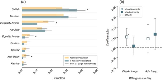
(a) Fractions of Distributional Preference Archetypes Based on the EET . (b) Coefficient Plots for the Dichotomous Variable Indicating the Finance Professional Subject Pool in Interval Regressions for Participants’ Willingness to Pay in the Domains of Disadvantageous and Advantageous Inequalities, Respectively.
Notes: In (a) the error bars indicate logit-transformed 95% confidence intervals; significance indicators are based on two-sample tests of proportion. Here |$n_{\it GP} = 395, n_{\it FP} = 298$|. In (b) hollow markers show estimates from models without adjustments (n = 693); solid markers show estimates from models with adjustment variables (n = 688). Error bars indicate 95% confidence intervals based on robust standard errors. The regression estimates are provided in Table C2 in Online Appendix C. |$^*\, p < 0.05.$|
Above and beyond the delineation of distributional preference types, the EET allows characterising the observed choice behaviour in terms of participants’ willingness to pay for an increase or decrease of the counterpart’s material payoff in the domains of disadvantageous (|$\text{wtp}\, ^d$|) and advantageous inequalities (|$\text{wtp}\, ^a$|), respectively. As such, |$\text{wtp}\, ^d$| (|$\text{wtp}\, ^a$|) can be interpreted as the monetary amount a decision-maker is willing to give up in order to increase (if |$\text{wtp}\, \gt 0$|) or decrease (if |$\text{wtp}\,$| < 0) the other player’s payoff by one unit in the domain of disadvantageous (advantageous) inequality.
Panel (b) of Figure 2 shows the coefficient estimates for the dichotomous variable indicating finance professionals in interval regressions for participants’ willingness to pay in the domains of disadvantageous and advantageous inequalities (as reported in Table C2 in Online Appendix C). With regards to the domain of advantageous inequality, we find that both subject pools tend to be benevolent toward their counterpart when they are ahead in terms of material payoffs. We do not find evidence for differences in participants’ willingness to pay (|$\text{wtp}\, ^a$|) between subject pools in this domain of inequality. Turning to participants’ willingness to pay in the domain of disadvantageous inequality we find that finance professionals tend to have a slightly higher willingness to pay (|$\text{wtp}\, ^d$|) when they are behind in terms of material payoffs as compared to participants from the general population. This mirrors our earlier finding that financial professionals are less inclined to be inequality averse compared to participants from the general population. However, the magnitude of the effect is small (|$r_s = 0.093$|, |$\rm{95\% CI} = [0.019, 0.170]$|; |$p = 0.014$|) and the difference between subject pools vanishes if the model takes into account the heterogeneity in sociodemographic variables.14
2.3. Trust and Trustworthiness
Large sectors of the finance industry build on the foundation of trust (Zingales, 2015). For instance, financial advisory services call for clients’ trust in the consultant (Gurun et al., 2018; Burke and Hung, 2021)—not least due to information asymmetries, implying that clients cannot even assess the quality of the advice provided (Dulleck and Kerschbamer, 2006; Balafoutas and Kerschbamer, 2020). Moreover, stock market participation has been shown to be conditional on individuals’ trust in the finance sector (Guiso et al., 2008; Balloch et al., 2015; Georgarakos and Pasisi, 2015). While survey evidence indicates at best moderate levels of trust in the financial sector (Sapienza and Zingales, 2012; Holzmeister et al., 2022), we lack further evidence on prevalent trust in finance professionals, and whether the extent to which finance professionals are trusted is actually ‘justified’. Particularly little is known about the latter, i.e., finance professionals’ trustworthiness.15 A recent study by Gill et al. (2020) provided long-term causal evidence on lower levels of trustworthiness among college students who self-select into pursuing a career in the finance industry. These findings raise serious questions about the trustworthiness of finance professionals compared to the general population, thereby leading to the following research question: is there a difference in trustworthiness between finance professionals and people from the general population?
2.3.1. Method
To examine trust and trustworthiness, we implement a standard investment game (Berg et al., 1995),16 where participants are assigned to the roles of either the trustor (first mover) or the trustee (second mover). Trustors are endowed with 100 SEK and can forward between 0 and 100 SEK (in steps of 20 SEK) to the trustee, who receives three times the distributed amount. The trustee then decides how much of the tripled amount to return to the first mover (in steps of 20 SEK). We interpret the first-mover’s behaviour as indicating trust (in the trustee) and the second-mover‘s behaviour as indicating trustworthiness (Brülhart and Usunier, 2012).
In our setting, finance professionals were always assigned the role of the trustee, whereas participants from the general population were assigned one of the two roles at random: with a probability of two-thirds, they were the first mover, and with a probability of one-third, they were the second mover. To examine whether trust differs depending on whether the trustee is a participant from the general population or a finance professional, we assign first movers randomly into both conditions and tell them whether the matched player is a finance professional or a person from the general population. Since the matching of trustors and trustees was only implemented once all participants had finished the experiment, the second movers were required to decide strategically, i.e., they had to report how much they would return to the first mover conditional on each potentially received amount. Because of the asynchronous setting of our online experiment, we opted for the strategy method, bypassing the requirement that participants are matched in real time. Besides practical considerations, adopting the strategy methods entails the benefit that it results in more comprehensive experimental data, as one obtains observations even at nodes that are only reached occasionally in the actual course of game play. In case the trust game was chosen for payout, the payments for both roles were determined based on the decision of the second mover, which was conditioned on the decision of the randomly matched first mover.
2.3.2. Results
On average, participants from the general population acting as first movers entrust 69.3% (|${\rm SD} = 30.0\%$|; |$n = 105$|) of their endowment to trustees from the general population and 66.2% (|${\rm SD} = 31.1\%$|; |$n = 200$|) to trustees from the finance professional sample. The difference in the amounts sent to the second mover is not statistically significant between the two treatments (two-sample t-test: |$t(303) = 0.846$|, |$p = 0.3980$|; |$r_s = 0.049$|, |$\rm{95\% CI} = [-0.064, 0.163]$|).17
With regards to the second movers’ behaviour, we find that finance professionals, on average, tend to be less trustworthy than participants from the general population, as they return systematically less at all amounts sent by the first mover (see panel (a) in Figure 3). In ordinary least-squares regressions of the amount returned by the trustee for each amount sent by the first mover, we show that the coefficient for the dichotomous variable indicating finance professionals turns out to be significantly negative, even after adjusting for the variation in socioeconomic variables (see panel (b) in Figure 3 and the detailed regression results in Table D2 in Online Appendix D).
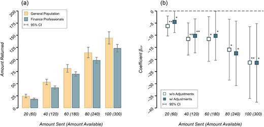
(a) Mean Amount Returned by Second Movers in the (Strategy Method) Trust Game Conditional on Each Possible Amount Sent by the First Mover, Separated for the General Population and Finance Professional Samples. (b) Coefficient Plots for the Dichotomous Variable Indicating the Finance Professional Subject Pool in Interval Regressions for the Amount Returned by Second Movers in the Trust Game for Each Amount Sent by the First Mover (the Tripled Amount Available is Indicated in Parentheses).
Notes: In (b) hollow markers show estimates from models without adjustments (n = 388); solid markers show estimates from models with adjustment variables (n = 387). Error bars indicate 95% confidence intervals based on robust standard errors. The estimates from the regressions are provided in Table D2 in Online Appendix D. |$^*\, p < 0.05,\ ^{**}\, p < 0.005.$|
Thus, our results suggest that finance professionals reciprocate trust (measured by the amount sent to them by the first mover) systematically less than participants from the general population. Importantly, this result prevails in comparable magnitude even when controlling for socioeconomic background variables. This finding is in line with the results of Gill et al. (2020) and resonates with perceived mistrust toward protagonists of the finance industry that is regularly encountered (Sapienza and Zingales, 2012).
2.4. Dishonesty Behaviour
The question of whether finance professionals tend to behave dishonestly has been widely studied and discussed, arguably not least due to a prevalent perception of misconduct among bank employees (Cohn et al., 2014; Zingales, 2015; Egan et al., 2019; Rahwan et al., 2019; Huber and Huber, 2020). In particular, the finding of Cohn et al. (2014) that finance professionals are more dishonest than others when being experimentally primed with their professional identity gained widespread attention. These results suggest that the culture prevailing in the banking industry leads to more dishonest behaviour. More recently, these findings have been questioned (Rahwan et al., 2019), which has led to a discussion revolving around questions concerning the replicability and the method of priming (see, e.g., Vranka and Houdek, 2015 and Cohn et al., 2019). We add to this discussion by asking the following research question: do finance professionals show a higher or lower tendency to exhibit dishonest behaviour compared to people from the general population?
2.4.1. Method
To address this question, we experimentally examine dishonest behaviour based on a design similar to Fischbacher and Föllmi-Heusi (2013): participants throw three simulated dice (see, e.g., Kocher et al., 2018 for an application of the procedure using computer-simulated die rolls) and report the sum of the observed pips (i.e., between 3 and 18). The participants’ payoff is the sum of reported pips, multiplied by a factor of 10 SEK. Thus, participants have a financial incentive to report a higher number of pips than the actual number realised by the three dice. Since the actual outcome of the simulated die rolls is known to the experimenters, the task allows determining a measure of misreporting on the individual level.
2.4.2. Results
We find that 90.6% of the general population and 94.6% of the finance professional sample report the realised number of pips truthfully. Only 5.5% (GP) and 3.7% (FP) over-report the number of pips, respectively, whereas comparably small fractions of participants under-report the actual number of pips (3.8% of GP and 1.7% of FP). The general population sample, on average, reports 0.144 more pips than shown (one-sample t-test: |$t(394) = 1.785$|, |$p = 0.075$|; |$r_s = 0.090$|, |$\rm{95\% CI} = [-0.009, 0.191]$|); finance professionals, on average, over-report by 0.104 pips (one-sample t-test: |$t(297) = 1.584$|, |$p = 0.114$|; |$r_s = 0.092$|, |$\rm{95\% CI} = [-0.022, 0.2091]$|). Given that participants’ reports do not significantly differ from the actual number of pips in both samples, it does not come as a surprise that the difference in misreporting between the two subject pools does not significantly differ from zero (independent sample t-test: |$t(691) = 0.369$|, |$p = 0.712$|; |$r_s = 0.014$|, |$\rm{95\% CI} = [-0.061, 0.089]$|).
In general, we find only very little cheating—among both the general population and finance professional samples—in our experiment. While there are several results reported in the literature that indicate preferences for truth-telling or costs of dishonesty (see, e.g., Abeler et al., 2014; 2019), the virtual absence of dishonest behaviour in our experiment appears to be striking. While we cannot provide a conclusive explanation for the absence of dishonest behaviour, two potential reasons come to mind. First, there is evidence that potential observability of dishonest behaviour can lead to less dishonest reporting (Abeler et al., 2019). However, we apply a similar procedure (using computer-simulated die rolls) as, e.g., Kocher et al. (2018). Second, we usually expect participants of online surveys to provide truthful answers, so that a norm of honesty might prevail. Third, the modus operandi—i.e., the distribution of invitations by SCB as the official statistical office and participants’ awareness that register data provided by SCB will be matched with the experimental data—might have influenced the overall level of dishonest behaviour. More important for our research agenda is that we do not find differences in individual preferences for honesty between finance professionals and the general population in our experiment. However, if the experimental procedure influences the overall level of dishonesty, a potential difference between subject pools might have become less salient.18
2.5. Personality Traits
As personal characteristics are an elusive concept, we confine our research on personality traits that are typically the focus of public debates: (i) socially undesirable characteristics (i.e., the ‘Dark Triad’, measuring narcissism, psychopathy and Machiavellianism), (ii) competitiveness and (iii) the habitual patterns of personality traits (Zillig et al., 2002) as a whole (i.e., the Big Five: openness, conscientiousness, extraversion, agreeableness and neuroticism). Despite public interest in the question of whether finance professionals differ systematically from people employed in other fields, only few scientific studies address certain aspects of personality characteristics of practitioners in finance. For instance, in two papers Kirchler et al. (2018; 2020) reported higher levels of competitiveness among finance professionals compared to students, academics and the general population, but lower levels compared to professional athletes. The trait of psychopathy is particularly relevant for financial decision-making, since it explains misbehaviour in taking risk on behalf of others (Jones, 2014) and gambling with the money of someone else (Jones, 2013). Furthermore, there is evidence on correlations between low neuroticism and high openness (as Big-Five personality traits) and risk-taking (Lauriola and Levin, 2001) in general. Brown and Taylor (2014) reported on the correlation between extraversion and openness and the levels of debt and assets held and Bucciol and Zarri (2017) showed that agreeableness is negatively associated with stock holdings (see Bucciol and Zarri, 2017 for further evidence on the impact of personality traits beyond the Big Five).19
Thus, if personality traits of finance professionals systematically differ from the rest of the population, this might well have an influence on decisions made within the finance industry, in particular on behalf of clients. We therefore ask the following research question: is there a difference in personality traits (i.e., Big Five, Dark Triad and competitiveness) between finance professionals and people from the general population?
2.5.1. Method
We elicit the Big-Five personality traits (openness, conscientiousness, extraversion, agreeableness and neuroticism) using the validated 10-item inventory introduced by Rammstedt and Oliver (2007). Moreover, we elicit the socially undesirable personality traits of narcissism, psychopathy and Machiavellianism using the 12-item Dark Triad inventory by Jonason and Webster (2010). Finally, we run a five-item questionnaire on competitiveness, based on the sub-module of the Work and Family Life Orientation questionnaire by Helmreich and Spence (1978). The scores for each trait are z standardised across the pooled sample, implying a mean of zero and SD of one for all measures of personality characteristics.
2.5.2. Results
Figure 4 summarises the differences in the various personality characteristics between participants from the general population and finance professional samples (based on the results of ordinary least-squares regressions of the various personality traits on a variable indicating the finance professional sample, as well as the full models including adjustments for participants’ socioeconomic characteristics reported in Table E4 in Online Appendix E). As illustrated in panel (a) of Figure 4, we find that finance professionals tend to score higher on all three socially undesirable traits captured by the Dark Triad inventory: narcissism (|$r_s = 0.091$|, |$\rm{95\% CI} = [0.017, 0.167]$|), Machiavellianism (|$r_s = 0.106$|, |$\rm{95\% CI} = [0.032, 0.183]$|) and psychopathy (|$r_s = 0.182$|, |$\rm{95\% CI} = [0.109, 0.264]$|). Importantly, once we adjust the differences between the two subject pools for the variation in socioeconomic characteristics, the effect sizes are attenuated: while the effects in narcissism and Machiavellianism scores are virtually set to zero, the difference in psychopathy is reduced by a third, but remains significant (|$r_s = 0.122$|, |$\rm{95\% CI} = [0.048, 0.200]$|).
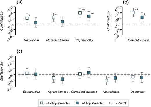
Coefficient Plots for the Personality Traits Elicited Using the (a) Dark Triad Inventory, (b) Competitiveness Items from the Work and Family Orientation Questionnaire and (c) Big-Five Inventory.
Notes: All panels depict estimates for the dichotomous variable indicating the finance professional subject pool in ordinary least-squares regressions. Hollow markers show estimates from models without adjustment variables (n = 693); solid markers show estimates from models with adjustments (n = 688). Error bars indicate 95% confidence intervals based on robust standard errors. The estimates from the regressions are provided in Table E4 in Online Appendix E. |$^*\, p < 0.05,\ ^{**}\, p < 0.005.$|
As outlined in panel (b) of Figure 4, we find that finance professionals, on average, tend to be significantly more competitive than participants from the general population. While this effect is in line with previous findings (Kirchler et al., 2018; 2020), the magnitude of the effect is rather small (|$r_s = 0.187$|, |$\rm{95\% CI} = [0.115, 0.270]$|) in our sample, and nearly halved (|$r_s = 0.105$|, |$\rm{95\% CI} = [0.031, 0.182]$|) by significant effects of gender, age and income (see Table E4 in Online Appendix E for details).
Finally, as illustrated in panel (c) of Figure 4, we do not find evidence on systematic differences between subject pools in terms of personality traits addressed by the Big-Five personality test. The only exception is a difference in neuroticism scores, which is of small magnitude (|$r_s = 0.098$|, |$\rm{95\% CI} = [0.023, 0.174]$|) and only to be found in the model not adjusting for socioeconomic characteristics. Once we control for participants’ socioeconomic background, the significant difference between subject pools is deflated.
Based on the analyses sketched above, we conclude that there is evidence for some differences between the two subject pools in our experiment. These differences are particularly pronounced before adding adjustment variables, pointing at sample characteristics of finance professionals. After adjusting for the socioeconomic background, we report that finance professionals tend to score higher on the psychopathy scale—a personality trait associated with untruthfulness, selfishness and being callous (see, e.g., Paulhus and Williams, 2002)—and tend to self-report being more competitive than participants from the general population. These results on competitiveness and psychopathy might emphasise the relevance of the question of a banking culture, as discussed above, and are consistent with a higher propensity of selfish behaviour among professionals that we find in our experiment (see Section 2.2).
3. Self-Selection, Industry Selection or Imprintment?
So far, we have shown that, without adjusting for participants’ socioeconomic characteristics, finance professionals are more risk-taking, more selfish, less inequality averse, show lower levels of trustworthiness and exhibit higher levels of narcissism, Machiavellianism, psychopathy and competitiveness. However, when controlling for differences in socioeconomic adjustments, we find that most differences vanish and that the prevailing findings on risk-taking, trustworthiness, psychopathy and competitiveness show lower effect sizes. For the remaining differences, however, the question about their origin arises. Can the differences between subject pools be explained by self-selection of professionals with certain characteristics into the industry, selection by the finance industry and/or imprintment of industry norms (i.e., the assimilation to industry-specific norms and its specific culture)?
To shed light on this question, we apply the following approach. First, we run additional analyses investigating the role of demographic variables, in particular gender and age, on behavioural differences across subject pools. Second, we run a survey, eliciting experts’ interpretation of our experimental findings. With this survey we analyse whether experts consider any of the three channels—industry selection, self-selection or imprinting—explanatory for the experimentally observed subject pool differences. Finally, we discuss implications derived from the experimental findings and the survey responses of the experts in this section.
3.1. Moderating Effects of Sociodemographics
To begin with, we analyse the role of demographic variables on behavioural differences between the two subject pools. We only consider age and gender as they are exogenous, whereas income and education are supposedly endogenous. In particular, we conduct ordinary least-squares regressions of the particular trait on an indicator variable for the finance professional subject pool (FP) and the socioeconomic adjustment variables (gender, age, income and education), extended by the interaction term FP |$\times$| age and FP |$\times$| gender. Up front we would like to note that the analyses below are post hoc and, accordingly, they should be interpreted with caution. In addition, analysing interaction effects sacrifices statistical power; thus, significant results might be exaggerated and insignificant results should be interpreted with even greater care.
The results of our analysis treating age as a moderator (left panels in Figure 5) show that the interaction effect FP |$\times$| age tends to narrow the difference between subject pools for all four characteristics. Yet, only the effect for competitiveness turns out being statistically significant: the effect of age on competitiveness differs between subject pools, as particularly young finance professionals are significantly more competitive than their non-finance counterparts.
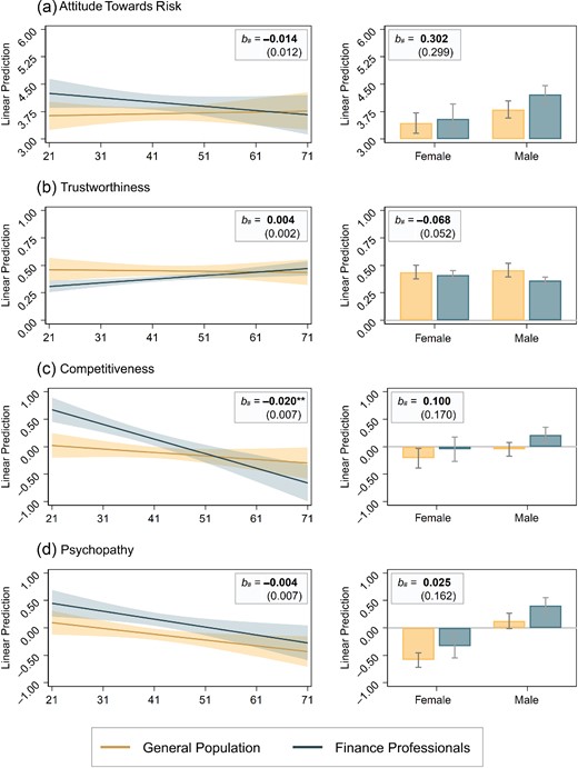
The Figure Plots Linear Predictions (and 95% Confidence Intervals) for (a) Attitudes toward Risk, (b) Trustworthiness, (c) Competitiveness and (d) Psychopathy Conditional on Age (Left Panels) and Gender (Right Panels), Separated for Finance Professional and General Population Samples.
Notes: Risk aversion enters in levels, competitiveness and psychopathy are standardised scores; trustworthiness enters as the average amount returned in percent across the five decisions in the strategy-method trust game (i.e., trustworthiness is percent scaled). The predicted margins are based on ordinary least-squares regressions of the particular trait on an indicator variable for the finance professional subject pool (FP) and the socioeconomic adjustment variables (gender, age, income and education), extended by the interaction term FP × age (left panels) and FP × gender (right panels). Here b# reported at the top of each panel presents the estimate of the interaction effect (with the corresponding standard error in parentheses). |$^{**}\, p < 0.005$|; n = 688 in all regression models.
Identifying why the gap narrows with age is difficult as the finding can be driven by self-selection in (and out) of the industry, selection by the industry itself or imprinting of industry norms. Using age as a proxy implies that people are exposed to industry norms for many years, which could be an indirect measure of imprintment of industry norms. However, it can also be the case that the prevailing culture in the finance industry has changed over time. In addition, age could also indirectly measure that professionals with different personality traits and preferences entered the industry decades ago—potentially because of different industry norms or different prerequisites from the industry. Therefore, we are cautious in the interpretation of the role of age for preferences and personality traits.20
Second, the finance industry is well known for its imbalance in terms of gender (Adams and Kirchmaier, 2016; Niessen-Ruenzi and Ruenzi, 2019). If differences between subjects pools observed in the experiment should be due to (industry or self-)selection effects, one would expect these differences to be larger for males than for females. As can be seen in the right panels of Figure 5, the interaction effect FP |$\times$| gender indeed tends to amplify the main effect (i.e., subject pool difference) for all four characteristics, although none of the coefficient estimates reaches statistical significance.
As for the analyses of the moderating effects of age, we are cautious in interpreting the moderating effects of gender. Gender can be considered as a coarse proxy for potential selection effects, either in terms of industry selection or self-selection into the industry. However, industry norms could—and probably will—interact with (industry and self-)selection, as purely male-dominated industry norms and a low fraction of female professionals might be unattractive for females to enter the industry. Therefore, in this analysis we cannot cleanly separate the roles of the different channels of selection into the industry or industry norms.
3.2. Expert Survey
3.2.1. Procedure
To circumvent the identification problems outlined in the previous subsection, we implemented a survey eliciting experts’ interpretation of our experimental findings (pre-registered at https://osf.io/5akcp).21 We obtained contact details of a pre-selected sample of experts from within the finance industry from SCB. We targeted human resource specialists (job code ‘2423’) and middle managers with personnel responsibility (job code ‘1612’) within the financial services (industry code ‘64’) and insurance industry (industry code ‘66’), respectively. In total, we contacted a random sample of 580 human resource specialists and 1,200 middle managers out of a total of 3,141 individuals that would have qualified as eligible participants. The contact details of this sample (postal addresses) obtained from SCB were forwarded to the third-party survey company Enkätfabriken, who generated and merged participant identifiers and login codes with the contact details for each participant and sent out the questionnaire during May 2022. As per the a priori power calculations, we aimed for 199 completes. Following our pre-registered stopping rule, we closed the survey after having reached this number of participants, leaving us with 205 complete observations. For completing the online survey, one out of 10 participants was randomly chosen and received 990 SEK for participation (provided as a gift card) via Enkätfabriken.
In the survey, participants were presented, in random order, with a description of the four tasks for which differences between financial professionals and the general population have been found after adjusting for the effect of variation in socioeconomic variables (i.e., attitudes toward risk, trustworthiness, competitiveness and psychopathy). For each of these tasks, participants were provided with a short description of the findings with regards to differences between financial professionals and participants from other industries.22 The survey was approved by the Internal Review Board at the University of Innsbruck.
For each of the four presented results, survey respondents were asked to indicate to what extent each of three potential explanations would likely account for the differences observed in the experiment. The three explanations (channels) were the following: (i) industry selection (‘Hiring decisions in the finance industry favor applicants with these characteristics.’); (ii) self-selection (‘People with these characteristics choose to work in the finance industry.’) and (iii) imprinting (‘The prevailing norms and culture in the finance industry over time influences the employees so that these characteristics become more common.’). For each of the three items (i.e., channels), subjects had to state to what degree the statements were correct using the following Likert scale: 1 (‘completely incorrect’); 2 (‘incorrect’); 3 (‘somewhat incorrect’); 4 (‘somewhat correct’); 5 (‘correct’); 6 (‘completely correct’). The order of the three items was randomised on the participant level to counter potential order effects (but remained constant for each participant to avoid confusion among respondents). For screenshots of the survey, see the pre-registration at https://osf.io/5akcp.
The goal of the expert survey is two-fold. First, the survey responses allow analysing whether or not experts with experience in hiring decisions in the finance industries consider any of the three channels (i.e., industry selection, self-selection or imprinting) explanatory for the observed subject pool difference for each of the four tasks. Second, the survey allows one to infer whether one particular channel is considered relatively more/less explanatory as compared to other channels for each of the four tasks.
3.2.2. Results
The mean survey responses, separated by the three channels, for the characteristics (i) attitudes toward risk, (ii) trustworthiness, (iii) competitiveness and (iv) psychopathy are illustrated in Figure 6. All tests based on the expert survey, as far as not otherwise indicated, have been pre-registered at https://osf.io/5akcp.
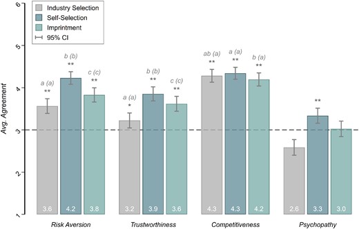
Average Survey Responses per Channel (Self-Selection, Industry Selection and Imprintment) for Attitudes toward Risk, Trustworthiness, Competitiveness and Psychopathy.
Notes: Survey questions were answered on a scale from 1 to 6. Error bars indicate 95% confidence intervals. Asterisks indicate statistical significance in one-tailed one-sample t-tests for |$\mu _0 = 3$| per channel per preference/trait type; |$^*\, p < 0.05,\ ^{**}\, p < 0.005$|; n = 205 in each test. Letters and letters in parentheses indicate significance groupings for pairwise comparisons between channels (that are statistically significantly larger than |$\mu _0 = 3$| in the one-sided tests) based on two-tailed paired-sample t-tests for p < 0.05 and p < 0.005, respectively (n = 205 in each test). That is, channels (per preference/trait type) with a common letter in the significance group label do not significantly differ in means.
In a first step, we examine whether or not experts consider any of the three channels explanatory for the observed differences between the finance professional and general population samples. We do so separately for each characteristic |$\times$| channel combination, by testing whether the mean level of agreement exceeds 3 (‘somewhat incorrect’) in a one-sided one-sample t-test, i.e., whether experts perceive a particular channel at least somewhat explanatory for the observed difference between subject pools in a particular task. Note that the statements were phrased as positive conjectures (e.g., ‘hiring decisions [...] favor applicants with these characteristics’). Choice options 3 (‘somewhat incorrect’) and 4 (‘somewhat correct’) divide the six-point scale into domains of agreement and disagreement. Thus, we interpret any choice exceeding 3 (‘somewhat correct’) on the scale to be indicative that a particular channel is at least somewhat explanatory for the differences observed in the main experiment. As reported in Figure 6, all three channels are perceived to play at least some role for the observed differences between subject pools for risk aversion, trustworthiness and competitiveness. For psychopathy, only self-selection is perceived somewhat explanatory, but not the industry-related channels of industry selection and imprintment.
In a second step, we investigate whether, for each of the four characteristics, any particular channel is considered relatively more or relatively less explanatory compared to other channels. For each task, we test whether responses differ systematically in pairwise comparisons of channels using (two-sided) paired-sample t-tests. The results are reported in Figure 6.23 For risk aversion and trustworthiness, the three pairwise comparisons between channels are significant at an |$\alpha = 0.5\%$| level; for competitiveness, only the difference between self-selection and imprintment turns out to be significant (|$p \lt 0.05$|), but the practical relevance is likely negligible. Notably, respondents’ average agreement is highest for self-selection into the industry for all four characteristics; imprintment ranks second and industry selection third in a horse race (except for competitiveness for which mean responses are approximately at par).
3.3. Discussion
The survey results shed light on the question of whether differences between subject pools are driven by self-selection, selection by the finance industry or industry imprintment from the perspective of experts who have an inside view into the finance industry. As such, the survey responses reveal several observations that allow for a more multi-faceted discussion of mechanisms potentially driving subject pool differences.
First, we observe that experts agree to a relatively large extent with the conjecture that differences between finance professionals and the general population are—at least partly—explained by the three channels, except for the difference in psychopathy. Conversely, respondents’ endorsement of the three channels suggests that experts in the field would expect finance professionals to differ from the general population in various characteristics due to the implications of self-selection, industry selection and imprintment that shape the industry.
Second, experts’ firm affirmation to all three channels indicate that they do not conceive self-selection, industry selection and imprintment to be mutually exclusive concepts: all three channels are considered relevant to explain the differences in attitudes toward risk, trustworthiness and competitiveness, but not psychopathy, between finance professionals and the general population. As such, the survey results are consistent with the assumption that the three channels are mutually correlated, probably even in a self-reinforcing manner. For the sake of illustration, suppose that people on average hold the belief that the finance industry endorses certain types of behavioural characteristics, say competitiveness and preparedness to take risk. This belief will translate into the expectation that competitive and risk-loving applicants will have an edge in the industry’s hiring processes, such that people will expect that the industry is indeed made up of competitive and risk-loving individuals. In turn, this expectation will presumably lead to a relative increase in applications from people who are willing to compete and take risks as compared to applications from less competitive and risk-taking candidates. As in the proverb ‘birds of a feather flock together’, individuals tend to associate and bond with similar others—a concept referred to as homophily (see, e.g., Lazarsfeld and Merton, 1954 and McPherson et al., 2001)—which can be expected to influence people’s choice of the industry (‘inbreeding homophily’; see, e.g., McPherson et al., 2001 and Currarini et al., 2016). Consequently, competition-seeking and risk-loving people will indeed be over-represented in the industry. The resulting proximity in terms of behavioural characteristics within the network could serve as a ‘breeding ground’ for a self-enhancing business culture (see, e.g., Charness et al., 2019 and Dimant, 2019). As employees tend to remain in the same industry for most of their working lives (Ellul et al., 2020), we can expect that they shape the industry (Gill et al., 2020).24 Managers with the mentioned risk preference and competitiveness are expected to more likely hire similar peers (see, e.g., Guenzel and Malmendier, 2020). Eventually, any of the steps in this chain of reasoning would feed back into the loop and would give people a good reason to strengthen their prior belief about the industry. The anticipation that industry selection, self-selection and imprintment shape the industry could suffice to make industry selection, self-selection and imprintment a self-fulfilling prophecy.
Third, we observe that different channels are still perceived to be explanatory to a varying degree for the different characteristics. As illustrated in Figure 6, experts conceive self-selection to be most relevant among the three channels to explain the observed differences in preferences and characteristics. Yet, we call for care when comparing the relevance of channels in a horse race based on our survey results: since the sample of respondents in our survey consists of human resource specialists and middle managers in the finance industry, they might be prone to motivated reasoning (see, e.g., Kunda, 1990), which would lead them to attribute differences in negatively connoted characteristics between finance professionals and the general population to self-selection rather than industry-related mechanisms (i.e., industry selection or imprinting). Given this potential limitation, the observation that industry selection is perceived to be at play for three out of four characteristics is even more remarkable, as it indicates that hiring decisions are not made to counteract the over-representation of employees that are more competitive, more risk tolerant or less trustworthy—despite the awareness of a lack of diversity in these characteristics.
4. Conclusion
With our study, we investigated differences in economic preferences and personality traits between a Swedish sample of finance professionals and a sample of the Swedish working population. In an online experiment, we assessed participants’ attitudes toward risk, losses and skewness, and elicited distributional preferences, trustworthiness, honesty and personality characteristics, including the Big-Five personality traits, the Dark Triad and competitiveness. The experimental data have been merged with registry data on socioeconomic characteristics provided by Statistics Sweden, which allows for adjusting the effects of interest for the variability of background variables.
First, we find that finance professionals are indeed different from the ‘average working adults’ employed in other industries, inasmuch as they are significantly less risk averse, more selfish, less trustworthy, more competitive and show higher levels of narcissism, psychopathy and Machiavellianism. Second, we show that after adjusting for socioeconomic background variables, finance professionals are not so different from a sample of the general population employed in other industries sharing a similar background: finance professionals ‘only’ tend to be slightly less risk averse, less trustworthy, show a slightly increased level of psychopathy and are more competitive than comparable participants from other industries. All other differences vanish and the magnitude of the effects remaining statistically significant tends to be deflated.
We would like to mention two points for discussion. First, although our analysis accounts for the variation in a number of socioeconomic characteristics, our adjustments are still limited (for reasons described in Online Appendix A). We cannot rule out that including additional information on participants’ socioeconomic background would not affect the observed (or not observed) differences between the finance professional and general working population samples. However, it is noteworthy that already a small set of standard socioeconomic characteristics entering our analysis as adjustment variables explains a substantial part of the differences between subject pools. In addition, self-selection into our experiment based on unobserved characteristics might affect our estimates (see Online Appendix A).
Second, our results provide hints where the differences in preferences and characteristics between finance professionals and the general working population stem from. Existing literature argues for both selection effects (e.g., Gill et al., 2020) as well as an influence (imprinting) from the industry (e.g., Cohn et al., 2014). It is difficult to disentangle selection into the finance industry on behalf of the industry and on behalf of individuals’ self-selection, as they are likely to be correlated with each other and with a prevailing industry culture. This raises the question about the distinction between selection and imprinting (industry culture norms). We therefore ran an experts survey with participants from the finance industry with hiring experience—human resource specialists and middle managers—to investigate whether they consider any of three channels, i.e., industry selection, self-selection or imprinting by industry norms, to be explanatory for the observed behavioural patterns. The results of the survey underline the idea that the three channels are mutually correlated: all three channels are perceived to play at least some role for the observed differences between subject pools for risk aversion, trustworthiness and competitiveness.
For these reasons, we would like to call for caution when interpreting observed selection effects as opposed to industry culture, because the latter can affect (self-)selection into the industry as well. This insight is also relevant when choosing where to set policy measures, because it shows that the selection of finance professionals into the industry might affect the peculiarities and culture of the finance industry, which, in turn, can lead to selection effects. Adams et al. (2016) surveyed the 2016 CFA membership and showed that female CFA members are less tradition and conformity oriented than male members. This suggests that gender-related barriers discourage women from entering the finance industry. Those barriers could, for instance, involve inflexible and/or long working hours, disadvantaging women facing more obligations outside their profession (e.g., due to child care). Goldin (2014) argued that long and inflexible working hours discourage women from self-selecting into industries where earnings have a non-linear relationship with respect to hours (see also Bertrand et al., 2010), which is particularly relevant for the legal, consulting and financial industries.
In tandem with the findings in our expert survey, this highlights the possibility of mutual correlations between the channels industry selection, self-selection and imprintment. This hints at possible policy measures, such as increasing the fraction of female professionals by changing the industry culture (e.g., flexible working hours, childcare facilities, mentoring programs). It can be expected that such measures would lead to increased self-selection of female professionals into the industry in the future. Further policy measures could already target increased university enrolment in relevant academic programs, as outlined by Adams and Kirchmaier (2016). If such interventions change the culture and in turn self-selection, in the long run we can also expect a transition in industry selection and screening (Gill et al., 2020). Maybe this is also what Christine Lagarde (president of the European Central Bank) had in mind when she said: ‘As I have said many times, if it had been Lehman Sisters rather than Lehman Brothers, the world might well look a lot different today.’25
Additional Supporting Information may be found in the online version of this article:
Online Appendix
Replication Package
Notes
The data and codes for this paper are available on the Journal repository. They were checked for their ability to reproduce the results presented in the paper. The replication package for this paper is available at the following address: https://doi.org/10.5281/zenodo.10122137.
We thank the Editor, Steffen Huck, and four anonymous reviewers for excellent comments and a very professional review process. We also thank Sebastien Duchene, Cary Frydman, Christoph Huber, Steffen Huck (the editor), Rudolf Kerschbamer, Christian König-Kersting, Stefan Palan and Julia Rose for very valuable comments on earlier versions of this paper. We particularly thank Fredrik Bergdahl and Ingrid Persson at Statistiska centralbyrån for the excellent collaboration on the project. Financial support from the Austrian Science Fund FWF (START-grant Y617-G11 and SFB F63), the Austrian National Bank (grant 17788), the Swedish Research Council (grant 2015-01713) and Formas (grant 2020-00199) is gratefully acknowledged. This study was ethically approved by the review boards at Statistiska centralbyrån (SCB; Statistics Sweden) and in Gothenburg (Sweden).
Footnotes
For instance, the share of the financial services industry in the gross domestic product in the United States was approximately 20% in 2019 (Bureau of Economic Analysis, https://bit.ly/39c9rHW; retrieved November 25, 2020).
See, for instance, the mediocre ratings for the banking industry in the United States during the last two decades: Gallup Business and Industry Ratings (http://bit.ly/3Jv4sU6, June 23, 2023).
Moreover, following the financial crisis of 2008, the tone of press coverage became substantially more negative; see Picard et al. (2014). Since our study has been conducted in Sweden, it is noteworthy that Sweden has also not been without scandals in the financial sector. For example, in 2020, one of the biggest banks, Swedbank, was found guilty and had to pay 4 billion SEK for money laundering in their Baltic subsidiaries. It was argued that the bank most likely suspected it, but did not take appropriate actions (see https://reut.rs/42PTwqY, April 9, 2021). In 2010, one of the largest Swedish bank crashes ever happened when HQ Bank was liquidated after it was found out that they were severely manipulating the values in the trading book in order to hide losses (https://bit.ly/3r7G5SF, April 09, 2021).
To name but a few examples, see Glaser et al. (2005), Pikulina et al. (2017) on overconfidence, Haigh and List (2005) on myopic loss aversion, Gilad and Kliger (2008) on risk priming, Kaustia et al. (2008) on anchoring, Cohn et al. (2014) on dishonesty, Kirchler et al. (2018) on social comparison and Holzmeister et al. (2020) on risk perception. For a recent overview of experiments with finance professionals, see Huber and König-Kersting (2022).
‘A financial analyst is responsible for a variety of research tasks in order to inform investment strategy and make investment decisions for their company or clients. This can include things like evaluating financial data, examining current events and market developments, examining an organization’s financial statements, and creating financial models to predict future performance.’ Retrieved from CFA Institute, July 11, 2022.
‘Investment adviser means any person who, for compensation, engages in the business of advising others, either directly or through publications or writings, as to the value of securities or as to the advisability of investing in, purchasing, or selling securities, or who, for compensation and as part of a regular business, issues or promulgates analyses or reports concerning securities.’ Retrieved from Legal Information Institute, July 11, 2022.
The experimental protocol has been registered at https://osf.io/r2fqn prior to the data collection.
In summary, we observe the following response patterns in our sample (note that the response rate refers to both the experiment reported in this paper as well as the accompanying experiment reported in Holzmeister et al., 2022 and Stefan et al., 2022). For the finance professional sample, the response rate analysis shows that men responded to a greater extent than women, and that finance individuals in the age group 45–59 years responded to a slightly lesser extent than other ages. For the general population group, the response rate analysis shows similar patterns regarding gender and age. We further observe a difference between the three job codes within the finance professional sample, where the response frequency was slightly lower (5%) in the group of traders and portfolio managers (job code ‘2414’) compared with analysts and advisers (code ‘2413’) and brokers (code ‘3311’) (6.4%).
At the time of the experiment, the exchange rate between USD and SEK was about 1:9; the exchange rate between EUR and SEK was about 1:10.5.
Extrapolating this number, the average hourly payout for the participants amounts to approximately $94 at the time of the experiment. This amount is comparable to other studies with finance professionals (e.g., Haigh and List, 2005; Kirchler et al., 2018) and general population samples (e.g., Andersson et al., 2016).
Note that we use only part of the available registry data. The main reason is that, for some of the registry data provided by SCB, we face substantial restrictions that are discussed in Online Appendix A. See Online Appendix A for further details on the register data.
We calculate standardised correlation coefficients per degree of freedom. For z statistics, the standardised correlation coefficient |$r_s$| is given by |$r_s = \tanh (z \cdot (n-3)^{-0.5})$|; for |$t(df)$| statistics, |$r_s = (t^2 \cdot (t^2 + df)^{-1})^{0.5}$| is applied. The 95% confidence intervals around |$r_s$| are determined by |$r_s \pm \tan (\arctan ^{-1}(r_s) - \Phi ^{-1}(0.975) \cdot (n-3)^{-0.5})$|, where |$\Phi ^{-1}(\cdot )$| denotes the inverse cumulative standard normal distribution function.
While our focus is on attitudes toward risk, skewness and losses, the symmetric 2|$\times$|2 variation across tasks also allows us to assess attitudes toward skewness in a mixed domain (including losses) or toward losses given skewed gambles, respectively. However, we only discuss these two types of attitudes parenthetically.
Note that the discrepancy between our results and the findings reported by Haigh and List (2005) and Abdellaoui et al. (2013) could be due to various reasons. For instance, the results could be specific to the samples (Haigh and List, 2005 recruited |$n=54$| ‘professional futures and options pit traders from the Chicago Board of Trade’; Abdellaoui et al. (2013) recruited |$n=46$| private bankers and fund managers from the United States and Lebanon) and/or specific to the experimental design (Abdellaoui et al., 2013 used a bisection method where subjects had to select one of two presented prospects varying in the payouts and the probabilities; Haigh and List, 2005 adopted the investment task of Gneezy and Potters, 1997).
As non-parametric robustness checks, we replicate the analysis based on participants’ |$(x,y)$| score, which constitutes an ordinal measure of distributional preferences and their intensities, using ordered logistic regressions (see panel (b) in Table C2 in Online Appendix C). It is reassuring that our results are qualitatively robust to the non-parametric measure.
There has been a discussion of the limitations of this investment game as a measure of trust. In particular, confounds, such as altruism (Cox, 2015) and betrayal aversion (Fehr, 2009), might dilute the observed behaviour in trust games, while at the same time other aspects of trusting behaviour might be neglected (Ermisch et al., 2009; Ben-Ner and Halldorsson, 2010). Since the investment game, arguably, remains the most popular experimental procedure to measure trust among researchers (Johnson and Mislin, 2011), we stick to this standard experiment, while we note cautiousness when it comes to interpreting the observed behaviour.
For further details on trusting behaviour, see Table D1 in Online Appendix D.
Note that we do not directly compare our findings to those reported by Cohn et al. (2014). The reason is that we do not examine the finance business culture and we can only provide little additional insight for this discussion, as our primary focus is on the comparison of individuals working in the finance industry and the general population. Thus, we have a different research question and a different methodological approach to Cohn et al. (2014).
For similar findings on stock market participation using the Temperament and Character Inventory instead of the Big-Five questionnaire, we refer the reader to Conlin et al. (2015).
Apparently, our analysis assumes that preference relations and personality traits are not rigid once they are formed, but rather can change over time. The psychological and economic literature indeed provides support for this assumption: for instance, previous studies provide evidence that personality traits change over the lifetime (see, e.g., Roberts et al., 2006 and Roberts and Mroczek, 2008), that willingness to take risk decreases with age (see, e.g., Dohmen et al., 2017 and Schildberg-Hörisch, 2018) and that trust increases as people get older (see, e.g., Sutter and Kocher, 2007). Since there is profound empirical evidence that preferences and behavioural traits can be unstable, it is not obvious that some characteristics would be better indicators for selection or imprintment than others. Even if traits and preferences might typically change at similar points in the life cycle, it cannot be ruled out that external factors—such as, e.g., exposure to a business culture or specific life events—could alter them as well.
For a related method, see Heinz et al. (2020).
We deliberately refrain (i) from giving an interpretation of the tasks and the measured preferences and characteristics (e.g., we did not use the word ‘psychopathy’), since the use of these terms may differ between everyday language and scientific use cases; and (ii) from providing statistical details, in particular effect sizes, since survey participants might lack the statistical skills to correctly interpret them. Moreover, participants might vary in statistical skills so that we could not have ensured consistent interpretation of statistical information across survey respondents. For these reasons, we provided a qualitative statement of differences and described them as systematic, a term we explicitly explained in the introduction to the survey.
Following our pre-analysis plan, we only test for differences in the relevance of channels if both channels (involved in a particular pairwise comparison) turn out to be statistically significant in the first analysis, i.e., if the means are significantly larger than 3 (‘somewhat incorrect’).
Our findings are consistent with those reported by Gill et al. (2020), since experts in our survey consider self-selection relevant for the findings on trustworthiness, while at the same time they acknowledge the importance of industry selection (and imprintment). Thus, our results can also be interpreted as evidence that the self-selection effect observed by Gill et al. (2020), i.e., that non-trustworthy graduates are more likely to self-select into the finance industry after finishing their studies, does not disappear over a professional’s life cycle.
Blog of the International Monetary Fund, available at https://bit.ly/3aDDcAm; retrieved February 2, 2021.
