


Abstract
We investigate how culture affects gender differences in willingness to compete in a large pre-registered experiment using an epidemiological approach. Our sample of 1,943 Norwegians with parents born in 59 different countries shows a smaller gender gap in willingness to compete among individuals of more gender-equal ancestries. The difference is driven by women with parents from more gender-equal countries wanting to compete more and men with the same ancestry wanting to compete less. The results are robust to controlling for a large set of factors at the individual, parental and ancestral country levels, indicating that gendered culture shapes competitive preferences.
The classic finding of Niederle and Vesterlund (2007) showing women being less willing to enter into competitions than men has survived countless replications (e.g., Niederle and Vesterlund, 2011; Niederle, 2017). Willingness to compete (WTC) is important because it explains part of the gender differences in educational choices and labour market outcomes (Buser et al., 2014; Flory et al., 2015; Reuben et al., 2019). We study how culture affects the gender difference in WTC in a large-scale, pre-registered online experiment with Norwegians whose parents were born in 59 different countries. We use female labour force participation (FLFP) in the parents’ countries of birth as a proxy for ancestral culture (often referred to as the epidemiological approach, e.g., Fernández and Fogli, 2009). Culture thus originates in the parental country of origin, is transported to Norway with migration and is reproduced within families via childhood socialisation.
Previous research suggests that cultural factors may be important for WTC, because there are large geographical variations in the gender differences. There are two opposing theories concerning individual gender differences in preferences and macro-level gender equality (Falk and Hermle, 2018). The resource hypothesis suggests that having more resources reduces barriers to gender-specific ambitions and goals, thereby increasing gender differences. Conversely, the social role hypothesis predicts that gender differences diminish in more gender-equal places as the views of women’s and men’s roles and positions in society become more equal. There are empirical studies supporting each hypothesis (e.g., Gneezy et al., 2009; Markowsky and Beblo, 2022). The best-known empirical example supporting the social role hypothesis comes from a seminal paper comparing selection into competition in a Masai society in Tanzania with selection into competition in a Khasi society in India (Gneezy et al., 2009). In these diverse locations, men compete more than women do in the patriarchal Masai community, while women compete more than men do in the matrilineal Khasi community. The result has been replicated in several studies and is generally interpreted as indicating that cultural differences connected to gender equality affect the gender difference in WTC (Andersen et al., 2013; Schwieren et al., 2020).1
One concern with interpreting differences in two settings is generalisability. For example, when comparing two other locations, Cárdenas et al. (2012) found that Swedish boys are more willing to compete than Swedish girls are, while in Colombia, they found no gender difference. As Sweden is ranked higher than Colombia in gender equality, the study thus supports the resource hypothesis. Similarly, several single-country studies in gender-equal countries such as Sweden and Norway have found gender differences in WTC (Boschini et al., 2019; Tungodden and Willén, 2023). In contrast, studies in less gender-equal societies find no gender differences in WTC (Khachatryan et al., 2015; Zhang, 2019). In fact, using data reported in Dariel et al. (2017), which includes data from 53 experiments conducted in 20 countries, we find that the gender differences in WTC are larger in countries with more gender equality.2
However, three problems arise when drawing conclusions from cross-country patterns. First, countries differ in institutions and endowments in addition to culture. Second, the selection of participants across countries may differ in a way that biases the results because male and female participants will be more or less representative of the population based on each country’s degree of gender equality. Third, experiments are often not set up in the same way across countries.
The epidemiological approach identifies the effect of culture while keeping institutions constant by comparing outcomes of individuals living in the same economic and institutional environment, but whose cultural beliefs, norms and preferences are potentially different due to different migration histories (Fernández, 2011; Giuliano, 2020). Using a classic competition experiment, we collected data online from 1,943 Norwegians with parents born in 59 different countries. As a proxy for ancestral culture, we use FLFP in the parents’ countries of birth (following, for instance, Fernández and Fogli, 2009). Our participants are born in Norway and other studies from Norway typically find a strong assimilating convergence from the first generation to the second (e.g., Finseraas et al., 2020). As such, all individuals in our sample face (comparatively) similar formal institutions, schools and labour markets, while differing in their cultural heritage from their parents. In other words, migration separates ancestral culture from the institutions that caused it.
Our main finding is that people whose parents are from more gender-equal countries have a smaller gender gap, where the difference is driven both by men with more gender-equal heritage being less willing to compete and by women with the same ancestry being more willing to compete. The gendered pattern of results suggests that gender culture affects gender differences in WTC, thus supporting the social role hypothesis. The gender differences in WTC remain after controlling for self-confidence and risk preferences, implying that preferences for competition drive the gender difference. Differential selection into the study does not seem to cause the effect of culture, and we find no differences in response rates across country backgrounds. A possible concern is that people with particular gender attitudes are more or less likely to migrate, though our approach partly controls for differential migration as long as these factors affect sons and daughters similarly. We also find clear positive correlations between gender attitudes reported in our survey and answers reported in the World Value Survey (WVS) of the parents’ home countries, suggesting that children have internalised attitudes from their parents’ ancestral countries through upbringing. A second possible concern relates to the variation in culture in our study sample. To increase power, our study oversampled individuals with parents from countries in the tails of the gender-equality distribution. A drawback of this approach, however, is that our results are most representative for the countries in the tails. In addition, all three oversampled countries with the lowest gender equality also have a high share of Muslims, making it difficult to separate egalitarian gender norms from religion.
Our main contribution is using the epidemiological approach to document the importance of the transmission of cultural beliefs and values for gender differences in WTC. Such cultural transmission is well documented with respect to fertility (Fernández and Fogli, 2009), trust (Guiso et al., 2006) and FLFP (Fernández, 2007; Finseraas and Kotsadam, 2017). However, to our knowledge, the transmission of beliefs and values regarding WTC has not been shown before. Compared to cross-country comparisons, a within-country study of culture ensures that the decision environment, level of payments and timing of the experiment are the same for all participants, and that no adjustments for purchasing power or translations are required. Additionally, the background variables, such as educational attainment, are comparable because they are from the same society (see Zhang, 2019 for similar arguments). Furthermore, we use data from high-quality administrative registers with minimal attrition and reporting problems, enabling us to investigate selection issues. Finally, our study is pre-registered.3
1. Experimental Design and Data
1.1. The Experiment
We follow the classical design of the competition experiment by Niederle and Vesterlund (2007), including several measures designed to parse out other differences between men and women, such as risk preferences, altruism and self-confidence. Our experiment consists of three rounds where the participants solve as many tasks as possible for 90 seconds and answer a survey. All participants received a show-up fee of 50 NOK, in addition to receiving payment for a randomly chosen part of the experiment (one of the three rounds or the survey part).
To reach the desired participant pool and the required sample size, we needed to recruit participants living in all parts of Norway. We therefore conducted the experiment as an incentivised online experiment, which means losing some control. For example, we cannot rule out respondents letting someone else answer in their place. However, in general, online experiments have previously been found to replicate laboratory experimental results (Horton et al., 2011; Edelman, 2012). The non-standard participant pool (see Section 1.4 for the definition of the population) makes our experiment an artefactual field experiment in the topology of Harrison and List (2004). We recruited respondents via text messages, inviting them to follow a link to a voluntary study where they could earn money.4 Data were collected between May and August 2019.
We modified two aspects of the classical design of Niederle and Vesterlund (2007) to conduct the experiment online: the task used and the composition of competition groups. The task in our experiment is counting the number of 1s in 5 × 5 matrices consisting of 0s and 1s (see Online Appendix Figure A.1). The task has two advantages. First, it reduces the possibilities of cheating in an online setting. Second, men and women have been found to perform equally well at this task in previous online experiments (Lezzi et al., 2015; Apicella et al., 2017; 2020).
In round 1 of the experiment, participants could earn 5 NOK (0.55 USD) for every task solved. In round 2, the competition round, payment was based on relative performance where player(s) with the highest performance within each group of four would receive a payment of 20 NOK per task. As in several recent studies, we informed participants that they would compete against the performance of three randomly drawn participants from an earlier pilot (e.g., Mayr et al., 2012; Burow et al., 2017 and Buser et al., 2020).5 After round 2, respondents were asked to self-assess their relative position in the group, where correct responses were incentivised with 5 NOK. This is a classic design solution assessing the importance of gender differences in self-confidence.
In round 3, participants performed the same counting task, but were asked to choose between the two payment schedules: either piece-rate payment as in round 1 or competitive payment as in round 2. This choice constitutes our main dependent variable measuring WTC. After making their decision, respondents started the counting task in round 3. Importantly, respondents who chose to compete, competed against the same group as in round 2. This approach both controls for altruism considerations and benchmarks payments against the performance of all participants in the group, not only those with a high WTC.
After completing round 3, participants were given a survey measuring several control variables, such as beliefs about their own performance, risk aversion and altruism (see Table 1 for all main variables and Online Appendix Section A.6 for the full questionnaire). We then informed respondents about which round was selected for payment, and how much they earned.
Definitions of Variables.
| (1) | (2) | (3) |
|---|---|---|
| Variable | Question | Coding |
| Risk | In general, how willing are you to take risks? | 1 = not willing to take risk at all; |
| ... 10 = very willing to take risk | ||
| Self-confidence | Guess of how well they performed in the counting task relative | |
| ... to the other group members | 1 = first place; 4 = fourth place | |
| Guess r1 | How many tasks do you think you solved in round 1 | continuous |
| Control | To what extent do you think your result in part 1 is due to controllable | |
| ... (i.e., effort) versus uncontrollable (i.e., chance and difficulty) factors? | 1 = no control; 10 = full control | |
| Gender attitudes scale | The average of these three variables: | 0: strongly agree; 1: agree; |
| 2: do not know; 3: disagree; | ||
| 4: strongly disagree | ||
| Being a housewife is just as fulfilling as working for pay | 0–4 (as above) | |
| On the whole, men make better political leaders than women do | 0–4 (as above) | |
| A university education is more important for a boy than for a girl | 0–4 (as above) | |
| Control | How much freedom of choice and control in life you have over the | |
| ... way your life turns out | 1: none at all, 10: a great deal | |
| Make parents proud | One of my main goals in life has been to make my parents proud | As gender attitudes |
| Live with parents | Do you live with your parents? | 1: yes, 0: no |
| Voted | Did you vote at the last election? | 1: yes, 0: no |
| Important to self | Which characteristics, if any, do you consider to be especially | |
| ... important to encourage children to learn at home?* | ||
| ... Gender equality | 1: listed characteristic; 0: did not list | |
| ... Religion | 1: listed characteristic; 0: did not list | |
| ... Willingness to compete | 1: listed characteristic; 0: did not list | |
| ... Hard work | 1: listed characteristic; 0: did not list | |
| ... Obedience | 1: listed characteristic; 0: did not list | |
| Important to parents | Which characteristics, if any, did your parents emphasise in your childhood?* | |
| ... Gender equality | 1: listed characteristic; 0: did not list | |
| ... Religion | 1: listed characteristic; 0: did not list | |
| ... Willingness to compete | 1: listed characteristic; 0: did not list | |
| ... Hard work | 1: listed characteristic; 0: did not list | |
| ... Obedience | 1: listed characteristic; 0: did not list |
Notes: *We ask respondents about what characteristics they think are especially important to encourage kids to develop. They can choose up to five characteristics out of 13. The 13 characteristics are independence; feeling of responsibility; imagination; tolerance and respect for other people; thrift, saving money and things; determination, perseverance; religious faith; unselfishness; obedience; politeness; gender equality; willingness to compete and hard work. We also ask the respondents what characteristics their parents focused on when they themselves grew up.
| (1) | (2) | (3) |
|---|---|---|
| Variable | Question | Coding |
| Risk | In general, how willing are you to take risks? | 1 = not willing to take risk at all; |
| ... 10 = very willing to take risk | ||
| Self-confidence | Guess of how well they performed in the counting task relative | |
| ... to the other group members | 1 = first place; 4 = fourth place | |
| Guess r1 | How many tasks do you think you solved in round 1 | continuous |
| Control | To what extent do you think your result in part 1 is due to controllable | |
| ... (i.e., effort) versus uncontrollable (i.e., chance and difficulty) factors? | 1 = no control; 10 = full control | |
| Gender attitudes scale | The average of these three variables: | 0: strongly agree; 1: agree; |
| 2: do not know; 3: disagree; | ||
| 4: strongly disagree | ||
| Being a housewife is just as fulfilling as working for pay | 0–4 (as above) | |
| On the whole, men make better political leaders than women do | 0–4 (as above) | |
| A university education is more important for a boy than for a girl | 0–4 (as above) | |
| Control | How much freedom of choice and control in life you have over the | |
| ... way your life turns out | 1: none at all, 10: a great deal | |
| Make parents proud | One of my main goals in life has been to make my parents proud | As gender attitudes |
| Live with parents | Do you live with your parents? | 1: yes, 0: no |
| Voted | Did you vote at the last election? | 1: yes, 0: no |
| Important to self | Which characteristics, if any, do you consider to be especially | |
| ... important to encourage children to learn at home?* | ||
| ... Gender equality | 1: listed characteristic; 0: did not list | |
| ... Religion | 1: listed characteristic; 0: did not list | |
| ... Willingness to compete | 1: listed characteristic; 0: did not list | |
| ... Hard work | 1: listed characteristic; 0: did not list | |
| ... Obedience | 1: listed characteristic; 0: did not list | |
| Important to parents | Which characteristics, if any, did your parents emphasise in your childhood?* | |
| ... Gender equality | 1: listed characteristic; 0: did not list | |
| ... Religion | 1: listed characteristic; 0: did not list | |
| ... Willingness to compete | 1: listed characteristic; 0: did not list | |
| ... Hard work | 1: listed characteristic; 0: did not list | |
| ... Obedience | 1: listed characteristic; 0: did not list |
Notes: *We ask respondents about what characteristics they think are especially important to encourage kids to develop. They can choose up to five characteristics out of 13. The 13 characteristics are independence; feeling of responsibility; imagination; tolerance and respect for other people; thrift, saving money and things; determination, perseverance; religious faith; unselfishness; obedience; politeness; gender equality; willingness to compete and hard work. We also ask the respondents what characteristics their parents focused on when they themselves grew up.
1.2. Data and Coding of Main Variables
We describe our data sets in more detail in Online Appendix Section A.7, which include data from our online competition experiment, Hauge et al. (2023), Statistics Faroe Islands (2005), Statistics Norway (2020), World Development Indicators Online Database (2020), World Economic Forum (2016), ILO (2014), World Value Survey (2015) and Dariel et al. (2017).
Our main dependent variable measures the WTC by the choice made in round 3. We code Compete to equal one if the respondent chose competitive remuneration and zero if piece-rate payment was chosen.
We use the standard measure within the epidemiological approach in economics (for a review, see Fernández, 2011) as our main pre-registered measure of egalitarian gender norms, namely, FLFP rates. We use those reported in the World Development Indicators online database for each country of ancestry in 2000.6 We measure FLFP in 2000 to have as complete coverage as possible for our countries of ancestry. In line with previous research using FLFP (Finseraas and Kotsadam, 2017; Finseraas et al., 2020), we use the natural log of FLFP to capture that a given percentage point difference in FLFP is likely more important at lower levels of FLFP. As seen in Figure 1, log FLFP generally correlates with other aspects of gender equality.
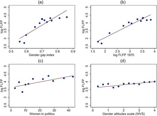
Comparison of Measures of Egalitarian Gender Norms.
Notes: The panels include binned scatter plots of log FLFP in year 2000: (a) the gender gap index, (b) log FLFP in 1970, (c) the share of women in politics and (d) the gender attitudes scale (from the WVS). Each dot represents a similar number of individual observations, and the lines are regression lines based on the full underlying data set.
We also include a second measure, namely, the World Economic Forum’s gender gap index (GGI) as a proxy for culture (see Online Appendix Section A.2 for details). GGI is available for only 52 of our 59 ancestral countries, whereas FLFP is available for all 59 ancestral countries. As seen in the upper-left quadrant of Figure 1, the two measures of culture correlate highly. In addition, log FLFP in 2000 is correlated with log FLFP in 1970, the percentage of women in politics and the gender attitudes reported in the WVS. In Table 1 we show the definition and coding of the gender attitudes scale, and of the other variables that we use from the survey, and in Table 2 we present descriptive statistics for all variables used in the regressions.
Descriptive Statistics.
| (1) | ||
|---|---|---|
| Mean | SD | |
| Main outcome variable | ||
| Compete | 0.33 | 0.47 |
| Other outcome variables | ||
| Performance under piece rate | 8.79 | 2.81 |
| Performance under competitive pay | 10.11 | 2.81 |
| Self-confidence | 2.19 | 0.92 |
| Risk | 6.14 | 1.98 |
| Control | 7.31 | 2.10 |
| Guess r1 | 7.52 | 4.48 |
| Main independent variables | ||
| FLFP | 57.78 | 24.17 |
| GGI | 0.72 | 0.09 |
| Background variables | ||
| Female | 0.55 | 0.50 |
| Education (years) | 15.34 | 2.69 |
| Mother's education | 13.84 | 3.85 |
| Father's education | 14.03 | 3.48 |
| Earnings (NOK) | 200,917 | 259,057 |
| Mother's earnings | 405,767 | 300,623 |
| Father's earnings | 538,374 | 462,426 |
| Married | 0.11 | 0.31 |
| Divorced | 0.01 | 0.11 |
| Widow | 0.00 | 0.00 |
| Single | 0.88 | 0.33 |
| Number of siblings | 2.27 | 1.51 |
| Household size | 2.64 | 1.57 |
| Birth year | 1,993.15 | 5.65 |
| N | 1,943 | |
Notes: This table reports means and SDs of the variables used in the regressions. The outcome variables are from our experiment, FLFP from the World Development Indicators online database, the GGI from the World Economic Forum and background variables from Statistics Norway.
1.3. Empirical Strategy and Hypotheses
We start by testing if there is a gender difference in WTC in the total sample and the extent to which the cross-ancestral country differences explain variation in female and male WTC separately. We then test if our proxy moderates the gender difference for egalitarian gender norms by estimating the following regression on the full sample:
That is, we regress WTC for individual i with country background c on a Female dummy, country fixed effects and Female × Culture. Our main measure of egalitarian gender norms (log FLFP) will be referred to as Culture from here on. Culture is standardised to have a mean of zero and an SD of 1. We expect that women will choose to compete less frequently than men; in other words, |$\beta$| is negative with a standardised measure of Culture. Here |$X_{i}$| is a set of birth year fixed effects, and we present results without the controls in the main text as pre-specified and with the controls in Online Appendix Table A.3.7 The error term |$\epsilon _{ic}$| is clustered at the country of the ancestry level.
The coefficient of interest is |$\lambda$|, and whether individuals with a background in more gender-egalitarian countries have a smaller or larger |$\lambda$| is treated as an open question. Given that |$\beta$| is negative, if we find that |$\lambda$| is positive (negative), it shows that the gender difference in competition is smaller (larger) for individuals whose parents come from a country with higher gender equality. Based on the gender-specific samples and tests, our main specified hypothesis is whether the Culture coefficient is statistically significant for either women or men, because the results would be interesting regardless of the interaction term being significant. Furthermore, the interaction term requires more power to be identified unless the effects go in opposite directions.
1.4. The Population and Sample
Our study population includes people born in Norway between 1980 and 2000 with at least one parent born outside of Norway in one of 59 different countries. We chose the 59 ancestral countries with the highest number of individuals recorded in the Population Register in Norway. The age group has a parent generation with a fair share of immigrants from various ancestral countries, giving us enough potential participants to recruit from. In addition, restricting the age of the study population to be between 19 and 39 years old ensures that people in the sample are not too different from each other, while also avoiding adolescence and menopause, both of which affect WTC (Andersen et al., 2013; Flory et al., 2018). See Online Appendix Table A.1 for a list of countries and sample sizes in our study.
We aimed at recruiting up to 40 participants from each country background: 20 women and 20 men. We intended to invite a random draw of 200 people from each country-gender cell, but not all country backgrounds had 200 people with phone numbers registered in the Population Register. The smallest group had 71 people, and with expected response rates below 28%, our goal would not be possible. Therefore, we invited all people available from countries with fewer than 200 people registered with a phone number, and a random draw of 200 people from countries with more than 200 people registered with a phone number.
The distribution of the invited sample sizes by parental country of birth is shown in Figure 2. Panel (a) shows that we invited a random draw of 200 individuals from 31 country backgrounds, while there are considerably fewer individuals from some country backgrounds. Panel (b) shows that the sample sizes by country background seem unrelated to our main measure of Culture. Additionally, we oversampled individuals at the tails of the FLFP distribution to increase power (List et al., 2011).8 In total, 1,943 consenting respondents completed the competition experiment (round 3). The distribution of background country sample sizes in the final sample is illustrated in panels (c) and (d) of Figure 2.
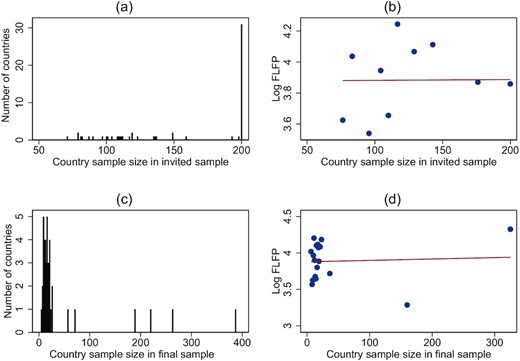
Sample Sizes by Ancestral Country.
Notes: The distribution of sample sizes by ancestral country, and the relation between sample sizes and log FLFP, in the invited sample and the final sample. Panels (b) and (d) are binned scatter plots, where the dots include similar numbers of individual observations and the regression lines are based on the full underlying data. Panels (a) and (b) include initial invitations and are therefore capped at 200 individuals. Because we invited more people from six countries, there are countries with over 200 individuals in panels (c) and (d).
2. Main Experimental Results
In this section, we present the basic experimental results.
2.1. Gender Difference in Performance and WTC
Replicating the findings of Lezzi et al. (2015) and Apicella et al. (2017; 2020), there is no significant gender difference in the respective performances (number of correct counts) of men and women in the counting task. In the piece-rate task (round 1), men reported on average 8.73 correct answers and women 8.84. In the competition task (round 2), men reported on average 10.02 correct answers and women 10.18. As can be seen from Table 3, these differences are not statistically significant. The distribution of performance is also very similar across gender (see Online Appendix Figure A.2).
Effect of Gender and Culture on Performance and WTC.
| (1) | (2) | (3) | (4) | (5) | (6) | (7) | |
|---|---|---|---|---|---|---|---|
| Performance piece rate | Performance competition | Compete | Compete | Compete | Compete | Compete | |
| Female | 0.108 | 0.156 | −0.139|$^{***}$| | −0.140|$^{***}$| | −0.139|$^{***}$| | ||
| (0.128) | (0.129) | (0.022) | (0.015) | (0.015) | |||
| Log FLFP | 0.021|$^{**}$| | −0.022|$^{*}$| | −0.022|$^{*}$| | ||||
| (0.009) | (0.012) | (0.012) | |||||
| Female × Log FLFP | 0.046|$^{***}$| | 0.044|$^{***}$| | |||||
| (0.012) | (0.012) | ||||||
| Mean dep. var. for men | 8.73 | 10.02 | 0.41 | ||||
| Mean dep. var. in sample | 0.27 | 0.41 | 0.33 | 0.33 | |||
| No. of observations | 1,943 | 1,943 | 1,943 | 1,067 | 876 | 1,943 | 1,943 |
| R2 | 0.00 | 0.00 | 0.02 | 0.00 | 0.00 | 0.06 | 0.02 |
| Sample | All | All | All | Women | Men | All | All |
| Country FEs | No | No | No | No | No | Yes | No |
| Mean FLFP | 57.78 | 57.78 | |||||
| SD FLFP | 24.17 | 24.17 |
Notes: Outcome variables are performance under piece-rate pay (performance piece rate) and performance under competitive pay (performance competition), measured as the number of correct answers, and WTC. Log FLFP is standardised with mean 0 and an SD of 1. SEs are given in parentheses. Robust SEs in columns (1)–(3) and SEs clustered at the ancestral-country level in columns (4)–(7). *p < 0.1, **p < 0.05, ***p < 0.01.
In column (3) of Table 3 we show the gender difference in WTC for the whole sample. While 41% of the men choose to compete, only 27% of the women do so. The difference is statistically significant and shows that women are 34% less likely to compete than men, which is comparable to previous studies in Norway (Tungodden and Willén, 2023) and Sweden (Boschini et al., 2019). Our survey measures of WTC show the same gender differences and correlate with our behavioural measure; see Online Appendix Section A.3.
In Figure 3 we show the relationship between performance and WTC as well as earnings from round 3 for men and women. The left-hand panel shows that WTC increases with performance for both men and women, but more so for men, which is consistent with the result in Buser et al. (2017). The right-hand panel shows the relation between performance in round 1 (piece-rate payment) and earnings in round 3 (choice between piece-rate payment and competition). On average, there is no statistically significant difference in earnings between men and women in round 3. However, more men earn zero, and more men earn a lot. The participants randomly selected from the pilot performed better than did the average participant in the experiment. The chances of winning were thus low, and only 2.5% of the competing individuals won. The low winning percentage does not affect the results, because 41% of the competitors thought they would win.9
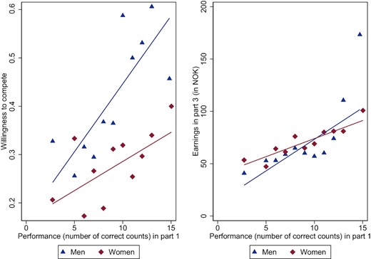
Relation between Performance, and WTC and Earnings.
Notes: The figure presents the relation between performance in the experimental task, measured as the number of correct answers (performance), and WTC and earnings in the experiment. The figures include binned scatter plots, where each dot represents a similar number of individual observations, and the lines are regression lines based on the full underlying data set.
2.2. The Effects of Culture on WTC
We expect that egalitarian gender norms affect WTC. Column (4) of Table 3 shows that the main measure of Culture is positively correlated with WTC for women. A one SD higher value of log FLFP (an SD in FLFP corresponds to around 24 percentage points) is statistically significantly correlated with a 2.1 percentage points higher WTC for women (p = 0.025). Column (5) shows that the correlation is reversed for men. Men with parents from countries with more women working are less likely to want to compete. The difference for men is statistically significant at the 10% level (p = 0.071). We thereby find support for our two main hypotheses, which were that egalitarian gender norms are correlated with WTC for women and men.10
In column (6), we show that our proxy for egalitarian gender norms moderates the gender difference. Using the full sample, we added country of ancestry fixed effects, and an interaction term between Female and log FLFP (note that the fixed effects subsume the log FLFP coefficient itself). For participants with parents from a country with an average level of FLFP (log FLFP is standardised to have mean zero), the gender gap in WTC is 14 percentage points. This gender gap is reduced by more than 30% in ancestral countries with a one SD higher FLFP. If we compare a country around the mean of the FLFP distribution (e.g., Hong Kong or Peru) with a country with a one SD higher FLFP (e.g., Denmark or Vietnam), we would predict a reduction in the gender gap of around one-third. Conversely, compared with a country with a one SD lower FLFP, such as India, we would expect an increase in the gender gap of around one-third. Column (7) shows similar results if we estimate the relationship without ancestral country fixed effects and instead include log FLFP. Figure 4 shows the results graphically in a binned scatter plot, where each bin contains on average 82 women or 67 men from 4.5 countries and the superimposed regression lines are based on the full underlying individual-level data. As such, each dot in Figure 4 does not represent individuals from one ancestral country background, but rather groups all individual observations into equally sized bins where one dot represents the average within one such bin. We note that the gap is never completely closed https://www.overleaf.com/project/628b7c2a26eca67a28828b1dlosed and in Online Appendix Figure A.3 we show the results using levels of FLFP. Extrapolating the results, we would see the gap closing at a FLFP of 140%.
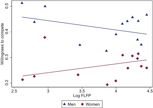
Relation between Culture and WTC.
Notes: The figure includes a binned scatter plot of our measure of Culture, log FLFP, in year 2000 and WTC by gender. Each dot represents a similar number of individual observations, and the lines are regression lines based on the full underlying data set.
These results are robust to various coding choices. In Online Appendix Table A.3, we show that the gender difference and effect of culture are very similar when adding year-of-birth fixed effects as additional control variables. The results are also similar when we interact year of birth with Female and Culture. We also ran a series of exploratory robustness tests (i.e., not pre-registered) showing that the results are similar when using levels of FLFP, if we take the difference between log female and log male LFP (Online Appendix Table A.4), if we use weights (Online Appendix Table A.5) and if we use FLFP from other years (Online Appendix Table A.7). In addition, both the gender difference and the effect of culture are stable in a series of regressions where one country is removed at a time (see Online Appendix Figure A.4). Our choice to oversample at the tails of the FLFP distribution means that our estimates have the highest external validity to the oversampled countries. We show in column 6 of Online Appendix Table A.8 that the results are not significantly different if we use a random sample of 40 individuals from the six oversampled countries instead of all observations from these countries. However, the point estimate is slightly lower and the standard errors increase. In summary, our results are not driven by age and seem robust to different coding of FLFP, and to which countries we include in the analysis.
Since we find a gender difference in the effect of ancestral culture on WTC, we are more confident that the observed relationship relates to gendered culture. As highlighted in Finseraas and Kotsadam (2017) and Finseraas et al. (2020), if the observed gender difference had remained constant across cultures, it could indicate something other than gendered culture affecting the results. It could still have been another aspect of culture, but the comparison across gender controls for all factors that affect men and women equally, such as non-gendered aspects of upbringing, parental networks and parental resources. Comparing men and women with the same ancestry further controls for omitted characteristics (e.g., work ethic) that correlate with ancestral FLFP and inherited outcomes, but are uncorrelated with gender. The variation retained is the part of ancestral FLFP that affects women and men differently. When using our complementary measure of culture, namely, the GGI, the relationship between culture and WTC shows a similar pattern as that shown in our main results, although less clear (see Online Appendix Section A.2).
2.3. Is Parental Ancestral Culture Internalised?
To investigate whether our sample has internalised the attitudes from their parents’ home countries, we compare responses given to the questions from the WVS in our survey with responses to the WVS for the overlapping 43 ancestral countries. We also investigate whether it matters if only one parent is born abroad or both.11 In column (1) of Table 4 we see that the answers given in our survey mostly correlate with the answers given to the same questions in the WVS in the ancestral country. As such, gender attitudes and several other attitudes and reported behaviours seem to be affected by ancestral egalitarian gender culture.
Correlations with Ancestral Country Measures.
| Correlation with WVS | Correlation with | |
|---|---|---|
| values in ancestor country | log FLFP | |
| Gender attitudes scale | 0.15|$^{**}$| | 0.10|$^{**}$| |
| Control | 0.07 | 0.16|$^{***}$| |
| Make parents proud | 0.35|$^{***}$| | 0.25|$^{***}$| |
| Live with parents | 0.89|$^{***}$| | −0.13|$^{***}$| |
| Voted | NA | 0.01 |
| Important to self | ||
| Gender equality | NA | −0.02* |
| Religion | 0.30|$^{***}$| | −0.08|$^{***}$| |
| Willingness to compete | NA | −0.02|$^{***}$| |
| Hard work | 0.11|$^{**}$| | −0.05|$^{***}$| |
| Obedience | 0.20|$^{***}$| | −0.02* |
| Important to parents | ||
| Gender equality | NA | 0.00 |
| Religion | NA | −0.17|$^{***}$| |
| Willingness to compete | NA | −0.00 |
| Hard work | NA | −0.02 |
| Obedience | NA | −0.03 |
Notes: The table includes correlations between answers from our survey and a) answers from the WVS, and b) our main measure of egalitarian-gender norms, log FLFP in year 2000. All variables are defined in Table 1. The table presents regression results using SE clustered at the ancestral country level. NA means the variable is not in the WVS. The number of observations in Column 1 is restricted due to countries not being included in the WVS and therefore ranges from 1,377 for the variable Live with parents to 1,703 for Obedience, Religion, and Hard work. In Column 2, we include the whole sample*p < 0.1,**p < 0.05,***p < 0.01.
An additional way to test whether ancestral culture influences gender attitudes is to examine the relationship between gender attitudes reported in our survey and log FLFP. As seen in column (2) of Table 4, log FLFP is strongly correlated with most other variables and, most importantly, it is positively correlated with the gender attitudes scale.12 In addition, individuals with parents from more gender-egalitarian countries put less emphasis on their children being competitive and developing gender-equal attitudes, perhaps because these individuals in our sample are already more gender equal. Our results are also in line with the results of Finseraas et al. (2020), which show that ancestral country FLFP is uncorrelated with voter turnout for Norwegians whose parents were born outside of Norway.
Earlier work has found signs of stronger vertical transmission of, for instance, religion in families where both parents share the same cultural background (Bisin and Verdier, 2011). If indeed parents transfer gender attitudes to children, the effect of culture should be stronger when both parents are born abroad than when one parent is born abroad and one is born in Norway. Table 5 displays the main culture effects separately for one parent born abroad (column (1)) and both parents born abroad (column (2)), showing no cultural effect for those with only one parent born abroad, while the effect is large for those with both parents born abroad. Cultural effects may be stronger for children with two parents born abroad because their parents value their ancestral culture differently, or because both parents represent the same ancestral culture. These regressions were not pre-registered.
Effect of Culture on WTC, Split by One or Both Parents Born Abroad.
| (1) | (2) | |
|---|---|---|
| Compete | Compete | |
| Female | −0.135|$^{**}$| | −0.102|$^{***}$| |
| (0.051) | (0.021) | |
| Female × Log FLFP | −0.015 | 0.078|$^{***}$| |
| (0.078) | (0.017) | |
| Mean dep. var. in sample | 0.35 | 0.32 |
| No. of observations | 1,075 | 816 |
| R2 | 0.08 | 0.11 |
| Sample | One | Both |
Notes: The outcome variable is WTC. Log FLFP is standardised with mean 0 and an SD of 1. SEs clustered at the ancestral-country level are given in parentheses.The regressions control for country fixed effects. **p < 0.05, ***p < 0.01.
3. Alternative Explanations
Having established a differential correlation between ancestral gender culture and WTC for women and men, in this section we investigate alternative explanations for our findings. In Section 3.1, we investigate the role of other factors at the individual and ancestral-country levels. In Section 3.2, we investigate the potential role of selection into the experiment.
3.1. General Factors at the Individual and Country Levels
It is common to investigate whether risk attitudes or self-confidence can explain the gender difference in WTC. Table 6 shows how including additional control variables affects the gender difference in WTC.13 While performance correlates with WTC, the gender difference is not related to performance, as seen in columns (1) and (2). Column (3) includes dummy variables for self-confidence, showing that individuals who did not believe they won (Believe 2nd, 3rd and 4th) want to compete less, but self-confidence explains only some of the gender gap. As seen in column (4), risk attitudes have little effect on the gender gap. There is a discussion in the literature about the role risk plays in driving the gender gap in WTC, and Gillen et al. (2019) argued that measurement error in risk measurement leads to biased conclusions. They further showed in their data that having several independent risk measures and using one of them to instrument for the other leads to different conclusions. We cannot conduct that type of analysis, because our study includes only one measure of risk. While we find that our measure of risk does not have much bearing on the gender gap, we caution against interpreting this result too strongly because measurement error, in part, may drive the result. Column (5) includes all control variables, still showing a substantial gender gap in WTC.
Effects of Culture on WTC, with Individual-Level Controls.
| (1) | (2) | (3) | (4) | (5) | (6) | |
|---|---|---|---|---|---|---|
| Compete | Compete | Compete | Compete | Compete | Compete | |
| Female | −0.141|$^{***}$| | −0.143|$^{***}$| | −0.106|$^{***}$| | −0.134|$^{***}$| | −0.108|$^{***}$| | −0.110|$^{***}$| |
| (0.021) | (0.021) | (0.021) | (0.022) | (0.022) | (0.017) | |
| Performance under piece-rate pay | 0.019|$^{***}$| | 0.006 | 0.006 | |||
| (0.004) | (0.005) | (0.006) | ||||
| Performance under competitive pay | 0.022|$^{***}$| | 0.006 | 0.006 | |||
| (0.004) | (0.005) | (0.005) | ||||
| Believe 2nd | −0.211|$^{***}$| | −0.203|$^{***}$| | −0.211|$^{***}$| | |||
| (0.028) | (0.029) | (0.024) | ||||
| Believe 3rd | −0.338|$^{***}$| | −0.323|$^{***}$| | −0.326|$^{***}$| | |||
| (0.029) | (0.031) | (0.031) | ||||
| Believe 4th | −0.337|$^{***}$| | −0.316|$^{***}$| | −0.318|$^{***}$| | |||
| (0.037) | (0.040) | (0.037) | ||||
| Risk | 0.020|$^{***}$| | 0.014|$^{**}$| | 0.016|$^{**}$| | |||
| (0.005) | (0.005) | (0.006) | ||||
| Control | −0.006 | −0.008 | ||||
| (0.005) | (0.006) | |||||
| Guess r1 | 0.000 | −0.000 | ||||
| (0.002) | (0.003) | |||||
| Female × Log FLFP | 0.053|$^{***}$| | |||||
| (0.019) | ||||||
| Mean dep. var. for men | 0.41 | 0.41 | 0.41 | 0.41 | 0.41 | 0.34 |
| No. of observations | 1,943 | 1,943 | 1,942 | 1,906 | 1,883 | 1,883 |
| R2 | 0.03 | 0.04 | 0.09 | 0.03 | 0.11 | 0.14 |
| Country FEs | No | No | No | No | No | Yes |
Notes: The outcome variable is WTC. Robust SEs are given in parentheses in columns (1)–(5) and SEs clustered at the ancestral-country level are given in parentheses in column (6). Log FLFP is standardised with mean 0 and an SD of 1. **p < 0.05, ***p < 0.01.
Column (6) of Table 6 includes the same control variables as column (5), in addition to an estimate of the effect of Culture (Female × Log FLFP). We note that culture may affect these control variables, introducing a possible post-treatment bias. Regardless, the effect of culture increases when including the controls.14 Hence, while individual differences explain part of the gender gap in WTC, they do not reduce the importance of culture. We show the effects of culture by gender in Online Appendix Table A.6, and in Online Appendix Table A.12 we present results for the main robustness checks using levels of FLFP, showing no effects of adding risk, performance and self-confidence. We repeat the same robustness tests using our secondary measure of culture, GGI, as the outcome variable, and the results are very similar (Online Appendix Table A.13).
The results show that culture affects the gender difference in WTC, implying that factors affecting women and men drive the results differently. However, it is interesting to see how other factors at the country level influence the gender gap, and whether the relationship between our main measure of culture and gender differences in WTC remains when controlling for the other factors. To investigate these matters, we add data on country-level education, the share of women in politics, GDP per capita and the share of different religions.
Table 7 shows results when we interact the country-level variables with gender (Female), including our main cultural variable (FLFP × Female). The regressions still control for country fixed effects, so the fixed effects subsume the country-level variables themselves. The cultural effect is stable, but the standard errors increase with the inclusion of Female × Muslims.15 Because the three oversampled countries at the bottom of the FLFP distribution are also countries with a high share of Muslims, we cannot separately identify the effect of FLFP when we control for Muslims × Female. These analyses were not pre-registered. Online Appendix Table A.8 shows that the effects are stable if we exclude one of these countries at a time, but the standard errors increase if we exclude all three of them.
Effect of Culture on WTC, With Country-Level Controls.
| (1) | (2) | (3) | (4) | (5) | (6) | (7) | (8) | |
|---|---|---|---|---|---|---|---|---|
| Compete | Compete | Compete | Compete | Compete | Compete | Compete | Compete | |
| Female | −0.137|$^{***}$| | −0.147|$^{***}$| | −0.141|$^{***}$| | −0.140|$^{***}$| | −0.141|$^{***}$| | −0.141|$^{***}$| | −0.140|$^{***}$| | −0.145|$^{***}$| |
| (0.015) | (0.019) | (0.016) | (0.015) | (0.015) | (0.015) | (0.015) | (0.021) | |
| Female × Log FLFP | 0.048|$^{**}$| | 0.067|$^{*}$| | 0.038|$^{*}$| | 0.047|$^{***}$| | 0.044|$^{**}$| | 0.039 | 0.049|$^{***}$| | 0.157|$^{**}$| |
| (0.023) | (0.034) | (0.020) | (0.012) | (0.017) | (0.061) | (0.012) | (0.073) | |
| Female × Years of schooling | 0.004 | 0.027 | ||||||
| (0.027) | (0.058) | |||||||
| Female × Women in politics | −0.022 | −0.081|$^{**}$| | ||||||
| (0.026) | (0.034) | |||||||
| Female × GDP pc 2000 | 0.014 | 0.007 | ||||||
| (0.023) | (0.057) | |||||||
| Female × Catholics | −0.001 | −0.002 | ||||||
| (0.016) | (0.034) | |||||||
| Female × Protestants | 0.006 | 0.028 | ||||||
| (0.019) | (0.042) | |||||||
| Female × Muslims | −0.008 | 0.089 | ||||||
| (0.062) | (0.101) | |||||||
| Female × Hindus | 0.023|$^{***}$| | 0.028|$^{**}$| | ||||||
| (0.005) | (0.012) | |||||||
| Country FEs | Yes | Yes | Yes | Yes | Yes | Yes | Yes | Yes |
| Mean dep. var. in sample | 0.33 | 0.33 | 0.33 | 0.33 | 0.33 | 0.33 | 0.33 | 0.34 |
| No. of observations | 1,802 | 1,613 | 1,858 | 1,890 | 1,890 | 1,890 | 1,890 | 1,566 |
| R2 | 0.05 | 0.06 | 0.06 | 0.06 | 0.06 | 0.06 | 0.06 | 0.06 |
Notes: The outcome variable is WTC. Log FLFP is standardised with mean 0 and an SD of 1. SEs clustered at the ancestral country level are given in parentheses. *p < 0.1, **p < 0.05, ***p < 0.01.
3.2. Selection into the Experiment
A concern in most lab experiments is whether the sample is representative. In our case, selection into the experiment may also bias the results if the selection is different for men and women from different countries. For example, if only highly educated women with parents from countries with low FLFP participate, while men of all educational backgrounds with the same cultural heritage participate, educational attainment would be a confounding factor.
As a first test of differential selection across cultures, we test if response rates correlate with our measure of Culture and whether they correlate differently for men and women. The smallest group available were women with parents from Afghanistan (31 individuals), so we invited 31 men and 31 women from each ancestral country background in the first week of the experiment. A variable was created, Response rate, for each group based on the percentage replying. Our pre-specified test is to regress the response rate on log FLFP for men and women separately, in addition to regressing it on Female, country fixed effects, and Female × FLFP for the full sample. Table 8 reveals that none of our variables correlated significantly with response rates.
Effects of Gender and Culture on Response Rates.
| (1) | (2) | (3) | (4) | |
|---|---|---|---|---|
| Response rate | Response rate | Response rate | Response rate | |
| Log FLFP | −0.001 | 0.008 | 0.008 | |
| (0.012) | (0.008) | (0.008) | ||
| Female × Log FLFP | −0.010 | −0.009 | ||
| (0.019) | (0.018) | |||
| Female | 0.016 | 0.017 | ||
| (0.027) | (0.026) | |||
| Mean dep. var. in sample | 0.10 | 0.09 | 0.10 | 0.10 |
| No. of observations | 1,243 | 1,015 | 2,258 | 2,258 |
| R2 | 0.00 | 0.03 | 0.34 | 0.04 |
| Sample | Women | Men | All | All |
| Country FEs | No | No | Yes | No |
| Mean FLFP | 56.56 | 56.56 | ||
| SD FLFP | 24.74 | 24.74 |
Notes: The outcome variable is Response rate. Log FLFP is standardised with mean 0 and an SD of 1. SEs clustered at the ancestral country level are given in parentheses.
We also kept track of how easy it was to get the respondents to answer. Assuming that there is a correlation between hard-to-reach respondents and non-respondents in their competitive behaviour, this correlation may teach us something about selection (Heffetz and Rabin, 2013; Heffetz and Reeves, 2019). Around 70% of our sample participated after receiving a reminder a couple of days after the first invitation. In Table 9, we show that there is a gender-gap and a culture effect for both early and late responders. Furthermore, the gender gap is larger for the late responders. Because late responders might be a better proxy for the effects among non-responders, this possibility implies that the effects may be larger than presented here.
Effect of Culture on WTC, Split by Answering the Survey Before or After the Reminder.
| (1) | (2) | (3) | (4) | (5) | (6) | |
|---|---|---|---|---|---|---|
| Compete | Compete | Compete | Compete | Compete | Compete | |
| Female | −0.166|$^{***}$| | −0.075|$^{*}$| | −0.075|$^{*}$| | −0.164|$^{***}$| | −0.080|$^{***}$| | −0.073|$^{**}$| |
| (0.026) | (0.039) | (0.039) | (0.021) | (0.030) | (0.028) | |
| After reminder | 0.076|$^{**}$| | 0.079|$^{***}$| | ||||
| (0.036) | (0.027) | |||||
| After reminder × Female | −0.091|$^{*}$| | −0.092|$^{**}$| | ||||
| (0.047) | (0.037) | |||||
| Female × Log FLFP | 0.049|$^{***}$| | 0.042|$^{**}$| | 0.038|$^{**}$| | |||
| (0.017) | (0.016) | (0.017) | ||||
| After reminder × Log FLFP | 0.044|$^{***}$| | |||||
| (0.016) | ||||||
| After reminder × Female × Log FLFP | 0.009 | |||||
| (0.027) | ||||||
| Mean dep. var. in sample | 0.43 | 0.36 | 0.41 | 0.34 | 0.32 | 0.33 |
| No. of observations | 1,361 | 582 | 1,943 | 1,361 | 582 | 1,943 |
| R2 | 0.03 | 0.01 | 0.02 | 0.07 | 0.10 | 0.06 |
| Sample | Late | Early | All | Late | Early | All |
| Country FEs | No | No | No | Yes | Yes | Yes |
| Mean FLFP | 57.64 | 58.10 | 57.78 | |||
| SD FLFP | 24.65 | 23.00 | 24.17 |
Notes: The outcome variable is WTC. Late refers to having answered after the reminder was sent and Early refers to having answered before the reminder was sent. SEs are given in parentheses. Robust SEs in columns (1)–(3) and SEs clustered at the ancestral country level in columns (4)–(6). Log FLFP is standardised with mean 0 and an SD of 1. *p < 0.1, **p < 0.05, ***p < 0.01.
To further investigate selection issues, we merge our survey data with information received from Norwegian administrative registers. Table 10 shows descriptive statistics of our sample compared with statistics of the target population living in Norway.16 Our sample has slightly higher education, as do their parents, than does the full population. Individuals in our sample have lower earnings, probably driven by a life-cycle bias, whereby individuals who stay in school longer have lower earnings at young ages. The samples have similar demographic characteristics.
Comparison of Experimental Sample and Population.
| (1) | (2) | |||
|---|---|---|---|---|
| Experimental sample | Population | |||
| Mean | SD | Mean | SD | |
| Education | 15.34 | 2.69 | 14.62 | 2.93 |
| Mother's education | 13.84 | 3.85 | 13.43 | 3.75 |
| Father's education | 14.03 | 3.48 | 13.60 | 3.51 |
| Earnings | 200,917 | 259,057 | 219,344 | 254,131 |
| Mother's earnings | 405,767 | 300,623 | 366,541 | 314,854 |
| Father's earnings | 538,374 | 462,426 | 462,569 | 549,544 |
| Married | 0.11 | 0.31 | 0.12 | 0.33 |
| Divorced | 0.01 | 0.11 | 0.02 | 0.12 |
| Widow | 0.00 | 0.00 | 0.00 | 0.01 |
| Single | 0.88 | 0.33 | 0.86 | 0.35 |
| Number of siblings | 2.27 | 1.51 | 2.17 | 1.52 |
| Household size | 2.64 | 1.57 | 2.61 | 1.46 |
| Birth year | 1,993.15 | 5.65 | 1,991.75 | 5.79 |
| N | 1,942 | 136,426 | ||
Notes: The experimental sample consists of the participants in our experiment and the population refers to all people living in Norway of the same ages and with parents born in the same countries.
We also test for selection effects by using the entire population for the age group in our study from the 59 countries in the registry data, and for each variable X in Table 10, we run regressions of the type
where Sample refers to our experimental sample and YoB is a set of year-of-birth fixed effects. Because log FLFP is standardised, |$\alpha$| gives us the difference between our sample and the total population sample for men from the country with average FLFP, and |$\kappa$| shows whether this difference is different for women. Both of these coefficients are interesting and important for external validity. The regression result also shows if there is differential selection for men, |$\psi$|, and shows the added differential selection for women, |$\lambda$|, both of which are important for the internal validity of the estimates. If |$\lambda$| is significantly different from zero, it would imply a differential selection of women as compared to men across cultures, even when country fixed effects are controlled for.
In Table 11, we see that |$\psi$| (i.e., the coefficient for Culture × Sample) is not statistically significant for any variable and that |$\lambda$| (i.e., the coefficient for Culture × Female × Sample) is statistically significantly different for only one variable, Divorced. However, it is very close to zero and one significant coefficient out of twelve is not concerning. Taken at face value, the result implies that women are more likely to have answered our study if they are divorced and are from countries with higher gender equality. In any case, we show in column 1 of Online Appendix Table A.15 that our results are robust when controlling for all the variables in Table 10, also when interacted with Female (column 2 of Online Appendix Table A.15).17 Compared with other women, married women are less likely to compete, which has not been reported in the literature before.
Tests of Differential Selection.
| Panel A. Selection tests using demographic variables | ||||||
| (1) | (2) | (3) | (4) | (5) | (6) | |
| Married | Divorced | Widow | Single | No. siblings | HH size | |
| Sample | 0.036|$^{***}$| | −0.001 | −0.000 | −0.035|$^{***}$| | 0.158|$^{***}$| | 0.046 |
| (0.010) | (0.002) | (0.000) | (0.010) | (0.050) | (0.051) | |
| Female | 0.037|$^{***}$| | 0.009|$^{***}$| | 0.000|$^{***}$| | −0.046|$^{***}$| | 0.007 | 0.059|$^{***}$| |
| (0.003) | (0.001) | (0.000) | (0.003) | (0.011) | (0.014) | |
| Log FLFP | −0.035|$^{**}$| | −0.005|$^{***}$| | −0.000 | 0.040|$^{**}$| | −0.401|$^{***}$| | −0.164|$^{***}$| |
| (0.015) | (0.001) | (0.000) | (0.016) | (0.097) | (0.043) | |
| Log FLFP × Sample | 0.009 | 0.001 | 0.000 | −0.010 | 0.040 | −0.038 |
| (0.007) | (0.003) | (0.000) | (0.007) | (0.053) | (0.060) | |
| Female × Log FLFP | −0.008|$^{**}$| | −0.003|$^{***}$| | 0.000 | 0.011|$^{**}$| | −0.058|$^{***}$| | −0.012 |
| (0.004) | (0.001) | (0.000) | (0.004) | (0.015) | (0.019) | |
| Female × Sample | −0.042|$^{***}$| | 0.001 | −0.000|$^{***}$| | 0.042|$^{***}$| | −0.080 | −0.118|$^{*}$| |
| (0.011) | (0.003) | (0.000) | (0.011) | (0.052) | (0.062) | |
| Log FLFP × Female × | 0.001 | 0.009|$^{**}$| | −0.000 | −0.010 | 0.030 | −0.053 |
| Sample | (0.008) | (0.003) | (0.000) | (0.008) | (0.057) | (0.054) |
| Mean dep. var. in sample | 0.12 | 0.02 | 0.00 | 0.86 | 2.17 | 2.61 |
| No. of observations | 137,900 | 137,900 | 137,900 | 137,900 | 137,930 | 119,395 |
| R2 | 0.17 | 0.03 | 0.00 | 0.21 | 0.08 | 0.11 |
| Panel B. Selection tests using education and earnings | ||||||
| (1) | (2) | (3) | (4) | (5) | (6) | |
| Education | Mother | Father | Earnings | Mother | Father | |
| Sample | 1.039|$^{***}$| | 0.349 | 0.483|$^{**}$| | 15,937.034|$^{**}$| | 36,840.619 | 79,794.073|$^{**}$| |
| (0.120) | (0.314) | (0.240) | (7,891.546) | (22,350.114) | (32,409.870) | |
| Female | 0.873|$^{***}$| | −0.009 | −0.006 | −41,631.475|$^{***}$| | 24.716 | 3,078.358 |
| (0.020) | (0.013) | (0.017) | (3,755.332) | (1,318.954) | (2,934.410) | |
| Log FLFP | 0.258|$^{***}$| | 1.174|$^{***}$| | 0.818*** | 3,080.925 | 68,132.299*** | 85,215.430|$^{***}$| |
| (0.062) | (0.281) | (0.213) | (4,366.818) | (12,143.080) | (15,755.918) | |
| Log FLFP × | −0.205 | 0.038 | −0.144 | −845.295 | 13,941.778 | 4,866.758 |
| Sample | (0.137) | (0.228) | (0.185) | (5,256.868) | (15,053.313) | (21,088.285) |
| Female × Log FLFP | −0.057|$^{***}$| | −0.015 | −0.002 | −897.746 | 1,569.797 | 4,504.574|$^{*}$| |
| (0.017) | (0.014) | (0.017) | (5,569.173) | (1,200.046) | (2,261.236) | |
| Female × Sample | −0.433|$^{***}$| | −0.018 | −0.166 | 15,903.161|$^{*}$| | −7,451.237 | −33,802.742|$^{**}$| |
| (0.154) | (0.157) | (0.121) | (9,403.485) | (14,800.470) | (16,585.358) | |
| Log FLFP × Female × | 0.161 | −0.113 | −0.135 | 3,688.048 | −7,234.593 | −14,376.006 |
| Sample | (0.136) | (0.133) | (0.108) | (5,893.578) | (12,089.920) | (10,965.852) |
| Mean dep. var. in sample | 14.63 | 13.44 | 13.61 | 219,043.22 | 367,165.51 | 463,664.94 |
| No. of observations | 122,107 | 120,777 | 118,524 | 137,931 | 131,017 | 130,232 |
| R2 | 0.08 | 0.10 | 0.05 | 0.31 | 0.07 | 0.05 |
Notes: Log FLFP is standardised with mean 0 and an SD of 1. SEs clustered at the ancestral country level are given in parentheses. All regressions control for year-of-birth fixed effects. *p < 0.1, **p < 0.05, ***p < 0.01.
Since culture is also likely to influence these demographic variables, potentially resulting in a post-treatment bias, the stability of the results reduces the concern that other important factors correlate with gender differences in behaviour and cross-country variations in gender culture. In particular, socioeconomic status could affect the behaviour of women and men differently, and we pre-registered testing if parents’ earnings constitute a threat for our analysis. Almås et al. (2015) found that kids in Norway from lower socioeconomic backgrounds are less willing to compete, which also interacts with gender. Specifically, they found that boys from lower socioeconomic status (SES) families compete less.18 In our sample, there is no interaction between gender and parental earnings to predict WTC, even when omitting other variables, as in column 3 of Online Appendix Table A.15, which reduces our concern that socioeconomic status affects the behaviour of men and women differently.
As for external validity, our sample is positively selected for education and earnings, after controlling for birth year fixed effects. Women are generally less selected than men are (Female × Sample), due to women having a higher response rate. Overall, we conclude that differential selection into the experiment is unlikely to drive our results.
Another type of selection is that parents immigrating to Norway may be unrepresentative of their country origins. However, our approach controls for differential migration from certain countries for specific reasons, as long as these factors affect sons and daughters similarly. If there is a more complicated selection process where more gender-equal individuals migrate to Norway from less gender-equal countries, our results are likely underestimated. If the reverse is true, that more gender-equal individuals migrate to Norway from more gender-equal countries, our results may be overestimated. It is impossible to know for sure what the selection process of immigrants to Norway looks like, but Norway is a country with a relatively compressed wage structure and comparatively low returns to education, which could lead to a negative selection of economic migrants for factors such as education (Borjas, 1991). Since education and egalitarian-gender norms correlate positively, one could expect the same to be true for gender equality. In addition, negative skill selection in OECD countries is stronger from culturally closer countries (Belot and Hatton, 2012). Our results from the analyses of the WVS data further show a clear correlation in the data between gender attitudes in the ancestral country and gender attitudes of the respondent, indicating that selection into migration does not play a major role.
A related concern is a differential selection of the parents of sons compared with the parents of daughters. Recall that all our participants were born in Norway and that the parents decided to migrate to Norway before participants were born. Only in cases where the mother was pregnant and knew the gender of the child before migrating could the gender of the future-born child influence the choice of migrating. We believe that it is unlikely that this type of differential selection is driving our results.
4. Conclusion
It is well known that women are less willing to enter into competitions than men are (Niederle and Vesterlund, 2011; Niederle, 2017), but less is known about where this difference originates from and what role culture plays in shaping this difference. In a series of influential studies, Gneezy et al. (2009) and Andersen et al. (2013) showed that women compete more in more gender-equal places. However, when comparing previously published data from studies across many countries, there is a positive correlation between macro-level gender equality and gender differences in WTC. This positive correlation is consistent with what Falk and Hermle (2018) call the resource hypothesis. When comparing across countries, it is unclear whether the observed differences come from differences in inherited preferences and beliefs (what we label culture) or from differences in reward systems and incentives due to different institutions or endowments.
In a pre-registered competition experiment with a large sample of Norwegian-born individuals, we find that the gender gap in WTC is lower for individuals with parents born in the more gender-equal countries. Both genders contribute to this pattern between ancestral culture and WTC, and the results are stronger if both parents are born abroad. We also find positive correlations between gender attitudes reported in our survey and answers reported to the same questions in parents’ home countries, suggesting that cultural differences transferred from parents to children through upbringing matter for gender attitudes. Our results are robust to individual-level factors that affect WTC, such as risk aversion and self-confidence, and ancestry-level factors unrelated to gender equality, such as levels of education or GDP per capita. Connecting data from the experiment to data from Norwegian administrative registers allows us to investigate selection effects more thoroughly than other studies have. While the participants in our experiment seem to be positively selected compared with the respective population in Norway, such selection effects do not seem consequential for our results, because there is little differential selection across gender in combination with culture. Our results are also robust when controlling for a host of variables at the individual level, including parental education and earnings.
Our results strongly suggest that culture matters for the gender differences in competitive preferences. However, we know from previous studies that institutions and policies also matter (Booth et al., 2018; Zhang, 2019), and that rules such as affirmative action and preferential treatment may reduce the differences (Balafoutas and Sutter, 2012; Niederle et al., 2013; Sutter et al., 2016). Our cross-country comparison of data from competition experiments from 20 different countries reported in Dariel et al. (2017) showed larger gender differences in WTC in more gender-equal countries (see Online Appendix Section A.4). This pattern is also found in a recent meta-study (Markowsky and Beblo, 2022). However, the cross-country evidence includes comparisons across countries with differences in cultures, institutions and resources, while the epidemiological approach holds institutions constant. Thus, the divergent results may stem from culture and institutions having different effects.
The different results could also be due to differences in the selection of lab participants across countries. For instance, female participants in a less gender-equal country might be less representative of the population of women in that country than are the male participants in the same country and the female participants from more gender-equal countries. Because many lab studies use university students as participants, there might be a concerning bias: because higher education among women is a function of the country-level gender equality, cross-country comparisons of studies where the samples are based on university students are conditioned on an endogenous variable.
Institutions and culture likely interact in creating gender differences (Alesina and Giuliano, 2015; Bisin and Verdier, 2017). We find differences along cultural lines in Norway, one of the most gender-equal countries in the world. Whether the effects of culture are different in other countries is an important and interesting question that we leave for future research. In particular, we urge researchers in the future to investigate the effects of culture in other settings using well-powered and pre-registered experiments to build up a credible evidence base on the role of both culture and institutions for gender differences.
Additional Supporting Information may be found in the online version of this article:
Online Appendix
Replication Package
Footnotes
Lowes (2018), however, does not find differences across matrilineal and patrilineal groups in the Democratic Republic of Congo.
See Online Appendix Section A.5 for a full description of the cross-country analysis.
The American Economic Association’s registry for randomised controlled trials (number AEARCTR-0004153).
The first text message read: ‘The University of Oslo and the Frisch Centre invite you to a research study. Contribute to research and earn 50–400 NOK. Voluntary, approx. 20 min’. Text message 2 (sent simultaneously with text message 1) read: ‘Read more about the research here: Link. Participate here (phone/tablet/computer): Link’. The reminder sent out two days later read: ‘We remind you about the invitation to participate in a research study. Your response is important for the research. Participate here: Link’.
We conducted a pilot of 40 students at the University of Oslo in the beginning of April 2019. We recruited participants through the mailing list of OECONLAB of students who previously have agreed to receive invitations to experiments.
https://databank.worldbank.org/data/home, variable SL.TLF.ACTI.FE.ZS. FLFP is the percentage of the female population aged 15–64 who are currently employed or seeking work. The underlying data are based mostly on labour force surveys. For Yugoslavia, we take the average of Bosnia and Herzegovina, and Croatia, which are the two former Yugoslavian countries in our sample. For the Faroe Islands, we use data from Statistics Faroe Islands (https://statbank.hagstova.fo/pxweb/en/H2/H2__AM/) for the year 2005.
To make the models fully saturated, we always partition the covariate space and add control variables as indicator variables rather than using their multi-valued coding (Athey and Imbens, 2017). If cells are too small, meaning less than 5% of the observations, adjacent cells are combined. When using interaction terms, we retain the continuous coding of the variables and standardise the variables for presentational purposes. For missing values on explanatory variables, we include results where we code the variables as zero and include dummy variables controlling for missing status, so that we do not lose observations.
Our pre-registered decision rule dictates that, if we were unable to obtain enough consenting participants from a country with a higher FLFP than the median (i.e., FLFP above 57), we invited additional participants from three other countries in the upper tail of the FLFP distribution with high numbers of potential participants. These three country backgrounds are Sweden, Denmark and Vietnam. If we did not get enough consenting participants from a country with a below-median FLFP (FLFP below 57), we would invite more individuals of the same gender from the three countries in the lower tail of the FLFP distribution with most potential second-generation respondents. These three countries are Pakistan, Somalia and Iran.
In Appendix Table A.9 we show some measures intended to capture the external relevance of WTC in our sample. Previous studies have shown that WTC correlates with earnings and education (Buser et al., 2014; Flory et al., 2015; Reuben et al., 2019). As seen in panel A, the correlation between choosing to compete and labour market earnings is relatively weak, perhaps due to the young age of our sample. Furthermore, WTC correlates with higher earnings for women. Panel B shows that WTC correlates positively, but very weakly and non-significantly, with years of education for both women and men. Finally, we show in panel C that WTC correlates with the probability of being enrolled in or having completed a science, technology, engineering and mathematics (STEM) higher education.
Also, when adjusting for testing two hypotheses using the false discovery rate method developed by Benjamini and Hochberg (1995), the hypothesis with the lowest p-value passes the test precisely because p = 0.025.
We also pre-registered that we would investigate if culture affects gender discrimination using a vignette experiment based on Finseraas et al. (2016). This vignette experiment presents candidates with different names (signalling gender), but with otherwise identical characteristics for a leadership position in a bank. The respondents are asked to evaluate how well they think the candidate fits the position, ranging from 1 = very poorly to 6 = very good, which we call Score. As we see in Online Appendix Table A.10, however, there is no baseline discrimination, because the female candidate (Ida in the vignette) is not given a lower score than the male candidate. There is no statistically significant relation between FLFP and getting the female candidate in the vignette in the total sample, or for men and women separately.
In column 5 of Online Appendix Table A.3, we see that women on average report more gender-equal attitudes than men do. There is a positive correlation between gender attitudes and culture, implying that men whose parents grew up in countries where FLFP was higher have more gender-equal attitudes. The coefficient for women is very similar, and gender difference in the effect of culture on gender attitudes is not statistically significant. Furthermore, as seen in Online Appendix Table A.11, there is no significant correlation between the gender attitudes scale and WTC (for either gender), nor does controlling for the scale weaken the effects of culture.
There exists several definitions of, and ways to measure, concepts related to confidence. Here we define self-confidence as the belief respondents held about how well they performed within the group (whether they came first, second, third or fourth). In a meta-analysis on overconfidence in experiments, Bandiera et al. (2022) defined confidence in relation to actual performance. In Online Appendix Section A.4, we include slightly different concepts of confidence following, among others, Apicella et al. (2017). We show there how risk attitudes and measures of self-confidence correlate with gender and culture.
The results are similar if we add an additional set of pre-specified controls in Online Appendix Table A.2, but these analyses make it hard to interpret the coefficients on overconfidence since several related variables are included. As seen in column 4 of Online Appendix Table A.3, the results are very similar when including dummy variables for missing observations.
We show the corresponding analyses for levels of FLFP in Online Appendix Table A.17.
We present a similar table for the six country backgrounds with the largest samples in Online Appendix Table A.14.
We show the corresponding analyses for levels of FLFP in Online Appendix Table A.16.
We pre-registered investigating if the observed pattern is consistent with the explanation in Almås et al. (2015) by asking the following questions. Is there a correlation between FLFP and SES (measured as parents’ earnings in the most recent year for which we have data)? Is the gender difference in competition negatively correlated with FLFP? Is the gender difference driven more by men than by women? If the answers to these three questions were all yes, it would indicate a problem in differentiating our cultural argument from the argument in Almås et al. (2015), meaning that we would then also control for parental earnings in additional regressions, despite problems of post-treatment bias. The answers to the questions are not yes, and the result holds up well when controlling for earnings and other variables. We also note that there is no interaction between gender and parental earnings predicting WTC in our sample.
Notes
The data and codes for this paper are available on the Journal repository. They were checked for their ability to reproduce the results presented in the paper. The authors were granted an exemption to publish parts of their data because access to these data is restricted. However, the authors provided the Journal with temporary access to the data, which enabled the Journal to run their codes. The codes for the parts subject to exemption are also available on the Journal repository. The restricted access data and these codes were also checked for their ability to reproduce the results presented in the paper. The replication package for this paper is available at the following address: https://doi.org/10.5281/zenodo.7787990.
We thank Kjell Arne Brekke, Åshild Johnsen, Johanna Möllerström, Gaute Torsvik, Oddbjørn Raaum, Eva Ranehill, Ole Røgeberg and participants at various seminars and conferences for useful comments. Funding from the Research Council of Norway (Grants No. 270772 and No. 250506/F10) is acknowledged. IRB approval was obtained at the Frisch Centre. An analysis plan is pre-registered at The American Economic Association’s registry for randomised controlled trials (No. AEARCTR-0004153) and all deviations from the plan are noted in the text.
