


Abstract
We develop a model of the politics of state capacity building undertaken by incumbent parties that have a comparative advantage in clientelism rather than in public goods provision. The model predicts that, when challenged by opponents, clientelistic incumbents have the incentive to prevent investments in state capacity. We provide empirical support for the model’s implications by studying policy decisions by the Institutional Revolutionary Party that affected local state capacity across Mexican municipalities and over time. Our difference-in-differences and instrumental variable identification strategies exploit a national shock that threatened the Mexican government’s hegemony in the early 1960s.
States with strong bureaucratic, fiscal and military capacities provide public goods and legal environments conducive to economic development and political stability.1 Yet many states lack these capabilities, especially in developing countries where clientelistic practices are ubiquitous.2 While there have been advances in understanding the sources of state capacity,3 we still lack a detailed understanding of its determinants in the presence of clientelism.
In this paper, we attempt to fill this gap in two ways. First, we develop a theory about how political incentives affect incumbent parties’ choices of how to build bureaucratic state capacity. We examine, in particular, incumbent parties that have a comparative advantage in providing transfers to their clients instead of providing public goods.4 Our model shows that investments in local bureaucratic state capacity that reduce the cost of providing public goods undermine the comparative advantage of incumbent clientelistic parties. As a result, these parties have an incentive to prevent such investments when threatened by increased political competition.
Second, we analyse the empirical implications of our model using a difference-in-differences (DiD) identification strategy that exploits a national shock that threatened the Institutional Revolutionary Party’s (PRI) hegemony in the early 1960s with varying intensity across municipalities. Following a decade of economic crisis, there was discontent in various sectors of the population with the PRI, weakening its clientelistic machine while strengthening opposition parties (Bartra, 1985).
To capture local bureaucratic capacity decisions by the PRI, we look at a land allocation program that transferred property rights to communities in the form of ejidos.5 This program redistributed more than |$50\%$| of Mexico’s agricultural land between 1910 and 1992 (Sanderson, 1984; Torres-Mazuera, 2009; Dell, 2012). Communities were often relocated to the allocated land. Since use rights were forfeited if the peasants moved away, individuals had incentives to remain in place (de Janvryet al., 2015). Importantly, national and state PRI governments chose where to locate the ejidos within each municipality.
Proximity to municipal headquarters was a central determinant of the cost of public good provision, and, consequently, of municipal bureaucratic state capacity. Official documents often point to the distance from their municipal headquarters as one of the main barriers to local public service delivery, and contemporaneous measures of such distance and service delivery exhibit a strong negative correlation.
Our theory predicts that increasing the distance of allocated ejidos from their municipal headquarters could be an advantageous strategy for an incumbent clientelistic politician facing increased political competition, as the PRI faced in the 1960s.
Our DiD identification strategy tests the model predictions by looking at changes over time in the distance of newly allocated ejidos from municipal headquarters across levels of political opposition.
Figure 1 provides a graphical intuition of our identification strategy and results. It shows two municipalities in the state of Durango that have roughly similar area and land available for redistribution, but that experienced different levels of political competition in the 1960s: low in the municipality on the left and high on the right. The plots in the top row depict land redistribution prior to 1960 and plots in the bottom row after 1960. In line with our model’s prediction, the ejidos allocated after 1960 were significantly farther away from the municipal headquarters in the municipality, where the PRI experienced a higher level of political competition. In contrast, those allocated before 1960 had a roughly similar distance from the municipal headquarters in both municipalities. DiD estimates confirm this graphical intuition: relative to before 1960, after 1960 the PRI strategically granted ejidos significantly farther away from municipal headquarters in places where it faced more political competition.
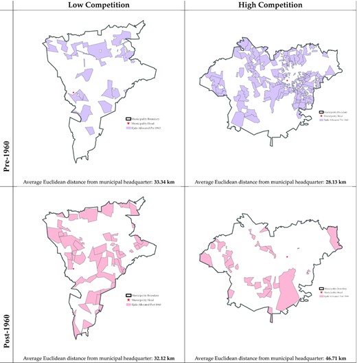
Allocation of Ejidos within Two Similar Municipalities in Durango.
Notes: Both municipalities belong to the same state (Durango), and are similar in area and land available for redistribution. High and low competition is defined based on whether the vote share for opposition parties is above or below the median.
The validity of our DiD estimates is supported by several exercises. In addition, we also use droughts during the 1950s as an instrument for our potentially endogenous measures of political competition within our DiD specification. Our IV-DID (Instrumental-variable-difference-in-differences) estimates confirm that the ejido distance increased after 1960 in more contested municipalities.
While we cannot rule out all other potential reasons for the documented patterns, we explore the most salient alternative interpretations of our findings by considering other outcomes and various heterogeneous effects.
Our paper primarily contributes to the literature on the determinants of state capacity. Several scholars study whether and how population density and inter- and intra-state conflicts have contributed to fiscal state capacity in Europe (Tilly, 1992; Gennaioli and Voth, 2015), Africa (Thies, 2007; Herbst, 2000; Sanchez de la Sierra, 2020) and Latin America (Centeno, 1997; Thies, 2005; Garfias, 2018).6 We extend this literature by studying the role that political competition plays in explaining choices that fundamentally influence local bureaucratic capacity in contexts where conflict did not lead to state capacity development. Recent articles by Acemogluet al. (2013) and Fergusson et al. (2016) study politician’s incentives to avoid eliminating non-state armed actors. While our paper shares an emphasis on political incentives to sustain state fragility, we focus on the bureaucratic ability to effectively provide public goods throughout the territory (Soifer, 2015; Henn, 2020), rather than on the monopoly of violence.
Lastly, our paper also speaks to the literature that highlights the negative effects of clientelism on public service delivery (Keefer, 2007; Hicken and Simmons, 2008; Fergusson et al.,2022). We contribute a new mechanism by emphasising the incentives to forestall investments in the local bureaucratic capacity.
1. Background
1.1. The Land Redistribution Program
A long history of land dispossession fuelled the agrarian discontent that contributed to the Mexican Revolution in the early twentieth century. Land distribution was thus at the centre of Mexico’s 1917 constitution. Land distributed to peasant communities in the form of ejidos was designated communal property, and therefore could not be sold, rented or used as collateral for credit. Individuals would lose inheritable (but otherwise non-transferable) use rights in the event of an extended absence.
Communities could request new land grants (dotaciones) or to have their land restituted (restituciones). We restrict our analysis to new land endowments, which constituted the bulk of the reform (see Online Appendix Figure A-1) and where authorities determined the location of new land endowments. Community demand was not the key factor that affected who got land and where it was granted. A highly centralised system gave the regime discretion over when and where to allocate land.
Ejidos became key to the PRI’s dominance because they facilitated the party’s clientelistic practices. The lack of individual property rights made peasants highly dependent on the government as the only source of agricultural credit, investments and technical assistance (Albertus et al.,2016). Also, its internal organisation, together with the PRI’s corporativist apparatus, facilitated the development of long-lasting clientelistic networks in communal lands (Larreguy, 2013; Sabloff, 1981).
The PRI’s decisions about where to distribute new land endowments had important long-term consequences for local bureaucratic state capacity since migrations from ejidos were infrequent. Once individuals were located on an ejido, they became ‘tied’ to their land, and thus unlikely to migrate (see Yates, 1981, p. 151, Fergusson, 2013, and de Janvry et al., 2015).
1.2. Social and Political Unrest and the PRI’s Response in the 1960s
The PRI’s power was essentially uncontested from the late 1920s to the late 1950s. However, the country’s vibrant post-revolution economic growth reached its limits in the late 1950s, which were characterised by general social discontent and protests from the main sectors of society previously under the control of the PRI’s clientelistic machine: industrial workers, students, teachers and peasants. This discontent was channelled into organised political opposition, which represented an important threat to the PRI’s hegemony in many areas of the country.
The rural sector was hit particularly hard by the economic crisis during the 1950s (Seageret al.,2009; Cerano Paredeset al., 2011). From the late 1950s until well into the 1960s, peasant movements surged throughout Mexico to express discontent and channel demands (Bartra, 1985). While peasants mobilised in rural areas, industrial workers and teachers also engaged in protests and strikes in urban centres (Herrera Calderón and Cedillo, 2012). The government usually responded by repressing protesters and incarcerating their leaders. Mexico’s political opposition absorbed this social discontent (Bartra, 1985). In the early 1960s, the PRI started to face strong threats from opposition candidates in several gubernatorial and municipal races. In response, the PRI engaged in election fraud (Bezdek, 1973). As a result, despite the increased political competition, the opposition won mayoral elections in only 17 out of approximately 2,400 municipalities and gubernatorial elections in one of the 31 states that held elections (Bezdek, 1973; Lujambio, 2001).
While the PRI’s fraud prevented the increase in political opposition from materialising in electoral competition in the short term, the threat of electoral competition persisted, as reflected by the association between municipal political discontent in the 1960s and political competition during the 1980s, that we show below. More importantly for our IV-DiD strategy, such municipal events and electoral competition correlate strongly with the droughts during the 1950s.
2. A Simple Model of State Building and Political Competition under Clientelism
2.1. Set-Up
We consider a model in the spirit of Robinson et al. (2006) and Robinson and Verdier (2013), in which an incumbent clientelistic (C) and an opposition non-clientelistic (NC) party compete for the rents from office R by deciding how much of an exogenously given budget T to spend on particularistic transfers (|$\tau$|) and public goods (g). The number of voters is normalised to one and there are two types of voters. An exogenously given |$\alpha$| share of voters—which we denote as clients(c)—are embedded in the clientelistic networks of the incumbent party, and so are targeted more efficiently with particularistic transfers. The remaining |$1-\alpha$| share of voters—which we denote as non-clients(nc)—can potentially benefit from particularistic transfers from the incumbent politician, but she cannot target them as efficiently. To capture that the incumbent has a comparative advantage in clientelism, we assume that the NC party is unable to provide particularistic transfers to voters, and is thus restricted to allocating the entire budget to public goods.7
The assumption that incumbent clientelistic parties have a comparative advantage in clientelism is central to the predictions of our model. This assumption has strong theoretical and empirical foundations. Incumbent parties are often better positioned to engage in clientelistic exchanges than opposition parties, due to greater access to the government resources usually used in clientelistic exchanges (de Kadt and Larreguy, 2018; Blattmanet al.,2019), which in turn makes their clientelistic promises more credible. Incumbents can also attract and incentivise high-performing political intermediaries since they represent better prospects (Bowles et al., forthcoming; Robinson and Verdier, 2013).
Using data from the Democratic Accountability and Linkages Project,8Online Appendix Table A-1 shows that incumbent parties across a large sample of countries are significantly more likely to engage in clientelistic practices than challengers.9
Finally, there is overwhelming evidence of the PRI’s comparative advantage in clientelism in our context (Magaloni, 2006; Larreguy, 2013; Larreguyet al.,2016), which allowed it to remain in power for more than seven decades.
2.2. Characterisation
2.3. Empirical Predictions
We next consider the incentive of the clientelistic incumbent to invest in bureaucratic state capacity and how this incentive depends on the political competition she faces.
The clientelistic incumbent’s pay-off may be increasing or decreasing in bureaucratic state capacity s.
The expression for |${\partial \Pi ^{C}}/{\partial s}$| in Proposition 1 shows that an increase in s, and the consequent fall in |$P_g(s)$|, produces two opposite effects: a ‘real-budget’ effect and a ‘relative-price’ effect. The ‘real-budget’ effect is due to an increase in the resources that the clientelistic incumbent may use to transfer benefits to its clients. The opposition candidate cannot use resources to target clients, and thus this first effect strengthens the incumbent’s electoral prospects and provides incentives to bolster bureaucratic state capacities. In contrast, the ‘relative-price’ effect—which is caused by a reduction in the cost of providing public goods—increases the public goods that the opposition party can provide, which hurts the incumbent’s electoral prospects.12
The overall impact of an increase in bureaucratic state capacity on the clientelistic party’s pay-offs therefore depends on which of these two effects dominates. While this depends on the value of the various model parameters, our empirical application focuses on the role of political competition, which we examine more closely in the next proposition. To mimic our empirical context, we model an increase in political competition as a decrease in the efficiency of the incumbent’s clientelistic machine.
Recall that |${\partial g^{C}}/{\partial \beta _c } = {P_{g}(s) }/{u^{\prime \prime }( g^{C})}.$| Substituting |$P_{g}(s)$| from (3) and using the definition |$\rho =-{g u^{\prime \prime }(g)}/{u^{\prime }(g)}$|, |$\beta _c {\partial g^{C}}/{\partial \beta _c }=-g^C / \rho$|. Substituting this into the cross derivative |${\partial ^2 \Pi }/{\partial s \partial \beta _c }=- P_g^{\prime } ( g^{C}+\beta _c {\partial g^{C}}/{\partial \beta _c }),$| and simplifying, we obtain the stated result.
The intuition for this result is the following. An increase in political competition faced by the incumbent party does not change the behaviour of the opposition party. Thus, the ‘relative-price’ effect of a reduction in s and the associated increase in |$P_g(s)$| is unchanged. However, increased political competition impacts directly and indirectly the ‘real-budget’ effects of a reduction in s because fewer resources are available for particularistic transfers. Directly, the cost of having fewer resources for transfers is lower with a more inefficient clientelistic machine. Indirectly, |$g^{C\star }$| increases when |$\beta _c$| falls, which increases the ‘real-budget’ cost of a reduction in s. As long as the direct effect is dominant, the incumbent prefers lower bureaucratic state capacity when it faces more electoral competition.
Proposition 2 states that this occurs if and only if |$\rho \gt 1$|, or in other words, when the utility from public goods exhibits sufficiently strong diminishing marginal returns. When this is the case, the incumbent clientelistic party provides fewer public goods because its marginal utility is lower. As a consequence, the indirect effect is not very large. Thus, the direct effect dominates, and the incumbent party prefers to strategically reduce bureaucratic state capacity. When |$\rho \lt 1$|, the reverse occurs, and contesting the power of the incumbent party causes the conditions for clientelism to gradually erode, as an increase in s and an associated fall in |$P_g(s)$| leads to a decrease in the provision of particularistic transfers.
Assessing whether |$\rho \gt 1$| is not feasible in our historical empirical context due to the lack of data and variation in incumbency, and to our knowledge, there are no measures of |$\rho \gt 1$| for public goods in the experimental and development literature. However, we compute estimates of |$\rho$| by exploiting the fact that |$\beta _c {\partial g^{C}}/{\partial \beta _c } = - g^{C} / \rho$|, and using estimates of the average |$\beta _c$|, |${\partial g^{C}}/{\partial \beta _c }$| and |$g^{C}$| from Larreguy (2013), who studied how the supply of education provided by the incumbent PRI across Mexico’s municipalities varies with the strength of the PRI’s clientelistic networks. Calibrations that take into account the number of schools, teachers and students indicate that |$\rho$| is comfortably above unity.13
We conclude by emphasising that the PRI could have responded to a surge in political competition by increasing ejido allocation in order to produce new clients (i.e., increase |$\alpha$|). However, increasing the number of ejidos is likely to have had a modest effect on the base of clients because land petitioners were likely to fall under the PRI’s corporatist apparatus anyway. More importantly, to show this possible complementary effect, we show below that land allocation did not increase more in competitive municipalities than in less competitive municipalities after 1960.
3. Data and Empirical Strategy
3.1. Data and Variables
Our empirical analyses require data from a variety of sources.14 We now describe the sources and computations for our main variables, with details about other variables given in Online Appendix Section A. The summary statistics are reported in Online Appendix Tables A-3 and A-4.
Our main outcome is the distance between the ejidos allocated between 1914 to 1992 from their municipal headquarters. We compute this distance for the 17,239 ejidos across 2,440 municipalities in our sample using spatial data on the mapping of ejidos to the localities—the smallest administrative divisions in Mexico—they contain, and the distance of localities from their municipal headquarters. Our baseline specification considers the minimum Euclidean distance of localities from their municipal headquarters.15
We consider two main measures of expected political competition. We first computed the vote share received by all opposition parties in the 1980s using mayoral electoral outcomes. Second, we used newspaper articles to code all events that described social and political discontent between 1960 and 1969, and we computed the (log) number for each municipality, both including and excluding rural events. This is original data collected from the two Mexican newspapers—Excelsior and El Universal—that had national coverage and were relatively uninfluenced by the national government.16 To instrument these measures of political competition, we use the number of months between 1950 and 1959 in which rainfall was strictly lower than the monthly long-run average in each municipality.
3.2. Empirical Strategy
A key implication of our model is that incumbent clientelistic parties should choose weaker bureaucratic state capacity when they expect greater political opposition. To test this prediction, we examine whether the PRI allocated ejidos further away from their municipal headquarters in municipalities where the party expected higher levels of political opposition.
Using the distance of the ejidos from their municipal headquarters to measure local state capacity decisions has several advantages. First, this distance persistently influences the local bureaucracy’s ability to provide the inhabitants of the newly allocated ejidos with public goods. Many government documents identify the distance of localities from their municipal headquarters as one of the main barriers for public goods provision and development (see, for example, Baja California State Government, 2003, p. 19; Secretariat of Social Development, 2014, p. 18; Gobierno de Mexico, 2007).
To reinforce this point, Online Appendix Table A-6 uses locality-level outcomes from the 1990 and 2000 Mexican censuses, to show that the distance of ejido localities from municipal headquarters is negatively associated with the provision of public goods by municipal governments even many years later, as captured by the share of households with piped water connections, drainage or electricity, as well as the number of active public schools per capita within 5 km of each locality.17
The second advantage of our measure is that the distance of the new ejidos from their municipal headquarters persistently influences local state capacity, given the inhabitant’s lack of geographical mobility. Therefore, it best captures the strategic choice to permanently increase the cost of public goods provision that we emphasise in our theory.
We consider two different measures of expected political competition: (a) opposition vote share, equal to |$1- {\mbox{(votes for PRI)}}/{\mbox{(total votes)}}$|, and (b) events of social and political discontent, equal to |$\log ( 1+ \text{events of discontent from 1960 to 1969}).$| To calculate the first measure, we use municipal electoral data during the 1980s for two reasons. First, while some municipal electoral results are available for the 1970s, these records are not complete, causing a concern that their availability is systematically correlated with the level of electoral competition and reducing the data available for the analysis. Second, the 1960s and 1970s saw significant electoral fraud, which we also expect to be associated with the electoral competition faced by the PRI. After the 1977 electoral reform, electoral figures are both fully available and much more reliable (Klesner, 1993).
We take the average opposition vote share across all municipal elections during the 1980s, reducing potential noise from specific elections.
Since this variable could be an outcome of the electoral threat that the PRI faced in the early 1960s, as a second measure of expected political competition, we use the number of events of social and political discontent between 1960 and 1969 in each municipality. Consistent with historical accounts, Online Appendix Figure A-6 shows that our two measures of political competition are strongly associated. This alternative measure is not subject to the same endogeneity concern.
Our identification assumption is that the ejido distance would have exhibited similar trends across municipalities experiencing varying degrees of political competition if the PRI had not experienced increased contestation in the 1960s. Similar trends in the ejido distance prior to 1960 support the plausibility of such an assumption. We also show that our results are not driven by variables that could be correlated with expected electoral competition, by verifying robustness to including interactions of a rich set of predetermined variables with time fixed effects. However, there remains a concern that our results are confounded by unobservable omitted variables.
4. Results
4.1. Baseline Results
We begin by graphically exploring our basic hypothesis together with the validity of our key identification assumption.
Figure 2 shows a plot with the coefficients of the interactions the opposition vote share in the 1980s with a full set of quinquennium dummies |$q_t$| (e.g., |$q_{1960}$| equals 1 if an ejido was allocated between 1960 and 1964) from regressions analogous to our baseline specification in (4). In this regression and all subsequent tables, we standardise the competition measure for ease of interpretation. These plots support both the validity of our similar-trend identification assumption and our hypothesis. Before 1960, when the PRI’s political power was not challenged, the interaction coefficients are close to zero and are statistically indistinguishable from those of the baseline quinquennium. However, starting in the 1960s, there is a differential increase in the ejido distance in municipalities with greater expected political competition.18
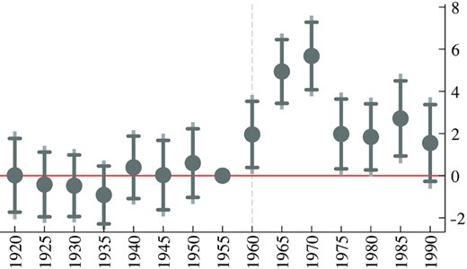
The Effect of Expected Political Competition (Opposition Vote Share) on the Distance of Ejidos from Municipal Headquarters.
Notes: Estimates, and 95% and 99% confidence intervals, of the regression of the distance of the allocated ejidos from their municipal headquarters on municipality fixed effects, quinquennium fixed effects, and the interaction of the standardised opposition vote share and the full set of quinquennium dummies. The omitted quinquennium is 1955 and represented by the coefficient without confidence intervals.
Table 1 reports the results of our OLS, IV-DiD and reduced-form specifications. Across both measures of political competition, the OLS-DiD estimates reported in column (1) are positive and statistically different from zero. A one-standard-deviation increase in the opposition vote share is associated with an increase in the distance of ejidos from their municipal headquarters after 1960 by about 3.243 km, or |$17.2\%$| of the sample average, a non-negligible increase. The coefficients for the events of social and political discontent imply a roughly similar effect: 2.391 km and 12.7%, respectively.19
Distance from Municipal Headquarters and Political Competition: OLS and Instrumental Variables.
| Baseline results, ejidos allocated from 1914 to 1992 | ||||
|---|---|---|---|---|
| (1) | (2) | (3) | (4) | |
| Dependent variable: | Distance of ejido from municipality head | Post-1960 |$\times$| competition | ||
| Econometric specification | OLS | IV | Reduced form | First stage |
| Panel A: competition measured as the vote share of opposition parties | ||||
| Post-1960 |$\times$| competition | 3.243** | 7.077*** | ||
| (1.308) | (2.717) | |||
| Post-1960 |$\times$| months with droughts during 1950–9 | 0.34*** | 2.43** | ||
| (0.05) | (0.99) | |||
| R2 | 0.579 | – | – | 0.621 |
| F-statistic (Kleibergen-Paap rk wald) | 38.99 | |||
| Observations | 17,059 | 17,059 | 17,059 | 17,059 |
| Panel B: competition measured as the number of events of social and political discontent during 1960–9 | ||||
| Post-1960 |$\times$| competition | 2.391** | 9.847** | ||
| (1.056) | (4.728) | |||
| Post-1960 |$\times$| months with droughts during 1950–9 | 0.21*** | 2.08** | ||
| (0.07) | (0.96) | |||
| R2 | 0.581 | – | – | 0.516 |
| F-statistic (Kleibergen-Paap rk Wald) | 9.518 | |||
| Observations | 17,239 | 17,239 | 17,239 | 17,239 |
| Controls for all specifications: | ||||
| Municipality fixed effects | |$\checkmark$| | |$\checkmark$| | |$\checkmark$| | |$\checkmark$| |
| Year of allocation fixed effects | |$\checkmark$| | |$\checkmark$| | |$\checkmark$| | |$\checkmark$| |
Notes: Robust SEs in parentheses are clustered at the municipality level, *** p|$\lt $|0.01, ** p|$\lt $|0.05. Regressions are at the ejido level. Competition refers to political competition measured at the municipality level using the variable indicated in each panel (see the notes to Online Appendix Table A-3 and the main text for exact definitions). All competition measures are standardised. The measure of droughts refers to the number of months from 1950 to 1959 in which the monthly rainfall was strictly lower than the long-run average of each particular month, and therefore accounting for seasonality and non-expected periods of low rainfall. The number of events reflecting social and political discontent are counted during the period 1960–9 using references to related events in two Mexican newspapers with national coverage: El Universal and Excelsior; further details are given in Online Appendix A.1. Distance of ejido from municipal headquarters refers to the population-weighted minimum Euclidean distance of the ejido localities from the municipal headquarters (see Online Appendix Figure A-3 for details).
The IV-DiD estimates reported in column (2) show somewhat larger estimates. For instance, the IV estimate suggests that a one-standard-deviation increase in the opposition vote share leads to a 7.07 km increase in the ejido distance after 1960, whereas the corresponding OLS estimate is 3.243 km. The reduced-form estimates in column (3) similarly indicate a positive and significant impact of droughts on the ejido distance after 1960. All these estimates robustly support the fact that increased expected political competition after 1960 led the PRI to locate ejidos further away from municipal headquarters.
Finally, positive and statistically significant first-stage estimates in column (4) confirm the historical accounts suggesting that the droughts during the 1950s contributed to social and political discontent and electoral opposition. Furthermore, the partialF-statistics support the relevance of our instrument. While the instrument in panel B is weaker than that in panel A, the F-statistic of the first stage is close enough to the rule of thumb of 10. Moreover, in subsequent robustness exercises, once we include time-varying controls, this statistic often becomes larger than 10.20
4.2. Robustness Exercises
One potential concern is that our DiD estimates reflect mean reversion or ceiling effects. For example, it is conceivable that the PRI allocated more land in municipalities that experienced more political contestation, possibly due to droughts during the 1950s. As a result, there would have been less land available for redistribution in these municipalities and the land that remained could well have been farther away from the municipal headquarters than in municipalities with less contestation. Our results could then be confounded by the municipal land available for redistribution and its proximity to municipal headquarters.
To empirically address ceiling effects, we run a specification where we include interactions of the post-1960 indicator with the stock of agricultural land available for redistribution by quartiles of distance from the municipal headquarters. We tackle mean reversion by including interactions with the amount of ejido land distributed by quartiles of distance from the municipal headquarters. We consider these interactive controls either at time t or in 1959.21
Panels A and C of Table 2 report the results of the specification in which we include the land available for redistribution at time t and in 1959, respectively. Panels B and D of Table 2 present analogous results when we instead control for interactions with the amount of ejido land distributed. Panels C and D deal with the concern that the controls at time t are ‘bad’ since they constitute outcomes (Angrist and Pischke, 2008). Reassuringly, throughout these specifications, the coefficients of the interaction with our political competition measures remain, not only significant, but also similar in size to those reported in Table 1.
Distance from the Municipal Headquarters and Political Competition: Accounting for the Area of Agricultural Land Available for Redistribution and Stock of Land Granted by Quartiles of Distance from the Municipal Headquarter.
| Dependent variable: distance of ejido from municipal headquarters | ||||
|---|---|---|---|---|
| (1) | (2) | (3) | (4) | |
| Competition measured as: | Opposition vote share | Events of social and political discontent | ||
| Econometric specification: | OLS | IV | OLS | IV |
| Panel A: controlling for the area of agricultural land available for redistribution by quartiles of distance from the municipal headquarters at time t | ||||
| Post-1960 |$\times$| competition | 2.945** | 6.133** | 2.188** | 8.564** |
| (1.323) | (2.566) | (0.961) | (4.322) | |
| R2 | 0.591 | 0.593 | ||
| First stage R2 | 0.630 | 0.522 | ||
| First-stage partial F | 41.06 | 11.29 | ||
| Panel B: controlling for the stock of land granted by quartiles of distance from the municipal headquarters up to time t | ||||
| Post-1960 |$\times$| competition | 2.912** | 6.541** | 2.134** | 9.243** |
| (1.313) | (2.644) | (0.988) | (4.538) | |
| R2 | 0.588 | 0.590 | ||
| First stage R2 | 0.628 | 0.520 | ||
| First-stage partial F | 40.52 | 10.67 | ||
| Panel C: controlling for the area of agricultural land available for redistribution by quartiles of distance from the municipal headquarters in 1959 | ||||
| Post-1960 |$\times$| competition | 2.320* | 6.092** | 2.323** | 7.923* |
| (1.231) | (2.843) | (0.981) | (4.276) | |
| R2 | 0.584 | 0.587 | ||
| First stage R2 | 0.637 | 0.522 | ||
| First-stage partial F | 38.98 | 11.40 | ||
| Panel D: controlling for the stock of land granted by quartiles of distance from the municipal headquarters in 1959 | ||||
| Post-1960 |$\times$| competition | 2.375** | 5.475** | 2.223** | 7.588* |
| (1.178) | (2.593) | (0.955) | (4.166) | |
| R2 | 0.584 | 0.587 | ||
| First stage R2 | 0.631 | 0.519 | ||
| First-stage partial F | 40.27 | 10.19 | ||
| Controls for all specifications: | ||||
| Municipality fixed effects | |$\checkmark$| | |$\checkmark$| | |$\checkmark$| | |$\checkmark$| |
| Year of allocation fixed effects | |$\checkmark$| | |$\checkmark$| | |$\checkmark$| | |$\checkmark$| |
| Observations | 17,031 | 17,031 | 17,207 | 17,207 |
Notes: Robust SEs in parentheses are clustered at the municipality level, ** p|$\lt $|0.05, * p|$\lt $|0.1. Post-1960 is a dummy variable that equals 1 if the ejido is granted after 1960. Competition refers to political competition measured at the municipality level using the variable indicated in each column. The IV columns instrument competition measures with the number of months with droughts during the 50s. The measure of droughts refers to the number of months from 1950 to 1959 in which the monthly rainfall was strictly lower than the long-run average of each particular month, and therefore accounting for seasonality and non-expected periods of low rainfall. The number of events reflecting social and political discontent are counted during the period 1960–9 using references to related events in two Mexican newspapers with national coverage: El Universal and Excelsior; further details are given in Online Appendix A.1. Land available is the fraction of land available for redistribution in the specified distance range from the municipal headquarters at year t. The land available excludes bodies of water and deserts. Stock of ejidos refers to the fraction of land redistributed in the form of ejidos in the specified distance range from the municipal headquarters. Further details on the construction of these variables are given in Online Appendix A-4. All independent variables are standardised.
Online Appendix B discusses four additional robustness exercises, all confirming our main conclusions. We investigate whether the increase in the distance of allocated ejidos varies with the nature of the political opposition (friendly or unfriendly) faced by the PRI; whether our estimates are biased by the strength of local rural elites; whether state-level confounders bias our results and whether results are sensitive to alternative measures of distance to the municipal headquarters.
5. Examining Alternative Interpretations
Our proposed mechanism—that the PRI located ejidos farther from municipal headquarters in an effort to weaken the local bureaucratic state capacity as a strategic response to increased expected electoral competition—might not be the only possible explanation for our main empirical results. We next assess the most salient alternatives.
5.1. Appeasing the Opposition
Possibly the most important alternative possibility is that increased competition led the PRI to increase ejido allocations in an effort to appease the opposition, which led to the distribution of marginal, lower-quality land located farther from municipal headquarters.
To assess the empirical relevance of this concern, we first test whether increased competition led to the allocation of more ejidos after 1960. We use the municipality year as the unit of observation and measure ejido allocation in different ways. In panel A of Table 3, we consider the number of allocated ejidos, in panel B the number of beneficiaries and in panel C the total area granted per beneficiary. The results across specifications provide no support for an increase in ejido allocations in more contested municipalities after 1960.
Amount of Land and Political Competition: Is It About Appeasing the Opposition?
| (1) | (2) | (3) | (4) | |
|---|---|---|---|---|
| Competition measured as: | Opposition vote share | Events of social and political discontent | ||
| Econometric specification: | OLS | IV | OLS | IV |
| Panel A: dependent variable: number of allocated ejidos | ||||
| Post-1960 |$\times$| Competition | −0.00 | −0.01 | −0.01*** | −0.01 |
| (0.00) | (0.02) | (0.00) | (0.02) | |
| Observations | 130,704 | 130,704 | 130,704 | 130,704 |
| R2 | 0.12 | 0.00 | 0.12 | 0.01 |
| First stage R2 | 0.466 | 0.469 | ||
| First stage F-statistic (Kleibergen-Paap rk wald) | 48.53 | 35.12 | ||
| Panel B: dependent variable: number of beneficiaries of ejidos | ||||
| Post-1960 |$\times$| competition | −0.08 | −0.89 | −0.71** | −0.97 |
| (0.30) | (1.56) | (0.35) | (1.69) | |
| Observations | 130,218 | 130,218 | 130,218 | 130,218 |
| R2 | 0.09 | 0.00 | 0.09 | 0.00 |
| First stage R2 | 0.467 | 0.470 | ||
| First stage F-statistic (Kleibergen-Paap rk wald) | 48.43 | 35.12 | ||
| Panel C: dependent variable: area granted in ejidos per beneficiary | ||||
| Post-1960 |$\times$| competition | −0.06 | −0.24 | −0.11 | −0.26 |
| (0.09) | (0.52) | (0.09) | (0.57) | |
| Observations | 130,220 | 130,220 | 130,220 | 130,220 |
| R2 | 0.06 | 0.00 | 0.06 | 0.00 |
| First stage R2 | 0.464 | 0.466 | ||
| First stage F-statistic (Kleibergen-Paap rk wald) | 47.09 | 34.27 | ||
| Controls for all specifications: | ||||
| Municipality fixed effects | |$\checkmark$| | |$\checkmark$| | |$\checkmark$| | |$\checkmark$| |
| Year of allocation fixed effects | |$\checkmark$| | |$\checkmark$| | |$\checkmark$| | |$\checkmark$| |
Notes: Robust SEs in parentheses are clustered at the municipality level, *** p|$\lt $|0.01, ** p|$\lt $|0.05. Regressions are at the municipality-year level. Post-1960 is a dummy variable that equals 1 after 1960, which is included in addition to the reported interaction term. Competition refers to political competition measured at the municipality level using the variable indicated in each column; see the notes to Online Appendix Table A-3 and the main text for exact definitions. All competition measures are standardised. The IV columns instrument competition measures with the number of months with droughts during the 50s. The measure of droughts refers to the number of months from 1950 to 1959, in which the monthly rainfall was strictly lower than the long-run average of each particular month, and therefore accounting for seasonality and non-expected periods of low rainfall. The number of events reflecting social and political discontent are counted during the period 1960–9 using references to related events in two Mexican newspapers with national coverage: El Universal and Excelsior; further details are given in Online Appendix A.1.
As we have anticipated, the lack of an effect on the extent of ejido allocations indicates that the PRI did not counteract a weakening of its clientelistic machine by simply creating more clients.22
5.2. Isolating Insurgents and Potential Opposition
Another alternative interpretation of our results is that they reflect the PRI’s strategy to deal with potential insurgents or citizen checks on the government, by relocating them to more isolated areas through the allocation of ejidos (Stasvage, 2010; Campante et al.,2019). This alternative interpretation seems unlikely since it implies an increased allocation of ejidos, which the results in Table 3 do not support. Nonetheless, we also test whether our estimates are larger in areas where the threat of insurgency was larger.
Online Appendix Table A-14 shows no heterogeneity in our main results by measures of social capital, population density or population of the municipal headquarters, which are factors shown to facilitate dissent.
5.3. Alternative State-Capacity Interpretations of our Distance Measure
To conclude, we discuss whether there might be dimensions of local state capacity other than the bureaucratic also affected by the distance of ejidos from municipal headquarters. First, it is unlikely that the ejido distance affected the state’s fiscal capacity. Because of the lack of individual property rights over ejidos, the ability of the Mexican state to tax peasants was indeed affected by ejido allocations (Torres-Mazuera, 2009), but this effect was independent of whereejidos were allocated.
Moreover, the increased ejido distance was not likely intended to increase the coercive reach and presence of the Mexican state in the frontier along the lines of Turner (1920). The process of state building in Mexico and Latin American differed greatly from that in the United States (García-Jimeno and Robinson, 2011). This alternative state capacity interpretation is at odds with the historical accounts and the basic patterns observed in our data. First, the Mexican state had its whole territory under control by the end of Lazaro Cárdena’s presidency in 1940 (Sánchez Talanquer, 2018). Second, the estimates in Online Appendix Table A-6 indicate that the allocation of ejidos far from municipal headquarters did not lead to increased local state presence, as captured by the relationship between the ejido distance to the municipal headquarters and contemporaneous measures of public service delivery; rather, it had the opposite effect.
6. Conclusion
Although state capacity is central to economic and financial development as well as to political stability and democracy, we still lack a definitive understanding of its determinants. A key observation in the recent literature is that, despite its benefits, investment in state capacity cannot be taken for granted, because political incentives often push political elites to forestall, rather than encourage, a stronger state. In this paper, we examine one such instance in the context of political clientelism. Since bureaucratic state capacity is a key determinant of the cost of public goods provision, investments in this area undermine the comparative advantage of incumbent clientelistic parties, which then have incentives to prevent strengthening state capacity in areas where their dominant political position might be threatened.
In addition to helping explain the determinants of state capacity choices in contexts where other theories fall short, our study also unveils the potentially perverse effect of political competition on economic development. In contrast to most conventional theories of the impact of stronger political competition, we find that, in areas where clientelism is prevalent, more electoral competition may deter state capacity strengthening, and by doing so, may impede economic development. While existing work highlights the benefits of political competition for public goods provision and more generally for economic development (Besley et al.,2010; Naidu, 2017), we argue that incumbent clientelistic parties may respond to increased political competition by hindering local bureaucratic state capacity and, consequently, public goods provision. Interestingly, these effects of political competition may be non-monotonic: if the competition is strong enough, the clientelistic party may be forced to change its strategy and also offer public goods (Diaz-Cayeros et al.,2016).
Additional Supporting Information may be found in the online version of this article:
Online Appendix
Replication Package
Footnotes
Throughout, we refer to ‘public goods’ as those that are not easily targeted to specific individuals or groups in the population. These contrast with what the literature on clientelism denotes as the ‘particularistic’ transfers that are targeted in exchange for political support (Kitschelt, 2000; Stokes, 2005; Hicken, 2011).
Ejidos were areas of land transferred to the community as a whole, where members had usufruct rights rather than private ownership rights.
Herbst (2000) argued that low population density limits the development of modern state institutions. Instead of taking population density as given and examining its implications, our work suggests that it can be endogenous to the political economy of state formation.
We abstract from commitment issues and assume that particularistic transfers can be credibly targeted to particular individuals in order to keep the discussion as simple as possible.
For more details, see https://sites.duke.edu/democracylinkage/.
For specific examples, see Stokes (2005) for the case of the Unity Party in Liberia, Magaloni (2006) and Larreguy et al. (2016) for the National Resistance Movement in Uganda and de Kadt and Larreguy (2018) for the African National Congress in South Africa. For the case of the Institutional Revolutionary and National Action Parties in Mexico, Blattmanet al. (2019) for the case of the Peronist party in Argentina, Bowleset al. (2020).
We will see that in equilibrium the incumbent party does not target any transfers to non-clients, and thus |$\beta _{nc}$| plays no role in determining the political competition faced by the clientelistic party. Here |$\beta _{c}$| is exogenously given and, while endogenising, it might be of theoretical interest, we consider an exogenous shift in our empirical application.
We assume that |$lim_{g\to 0} u^{\prime }( g) \to\infty$| and that |$u^{\prime }( T/P_g(s)) \lt P_g(s) \beta _c$| so that the interior condition holds.
This reduction in cost also increases the amount of public goods the clientelistic party may provide. However, according to the envelope theorem, the impact of an increase in s on the clientelistic party’s winning probability via the change in |$g^C$| is negligible. Note that the envelope condition does not hold for the opposition party, since it faces a corner solution.
We measure |$\beta _c$| considering the mean share of municipal land that belongs to an ejido, 0.234. We proxy for g using the municipal mean of schools, teachers and students, which are respectively given by 1.276, 8.343 and 191.6. The derivative |${\partial g^{C}}/{\partial \beta _c }$| is respectively given by −0.2857, −0.9697 and −25.08 for schools, teachers and students.
See Centro de Investigación para el Desarrollo A.C (CIDAC) (2012), Comision Nacional del Agua (CONAGUA) (2013), Food and Agriculture Organization (FAO) (2014), Gobierno de la República Mexicana (2011; 2013), Instituto Nacional de Estadística y Geografía (INEGI) (1990, 2000, 2007,2011, 2013), Secretaría de Gobernación (1994), Registro Agrario Nacional (2012), Kitschelt (2013), U.S. Department of Agriculture (2014).
In our robustness checks, we consider two alternative measures: we account for the elevation terrain profile by penalising our baseline distance when there are changes in altitude in the straight path and we measure the distance using roads. See Online Appendix Figure A-3 for a detailed explanation of the computation of these distances.
Online Appendix Figure A-5 presents the distribution of these events over time.
Such negative correlation holds for non-ejido localities, although it is marginally weaker.
We report the corresponding graph for the events of social and political discontent in Online Appendix Figure A-7.
Online Appendix Table A-8 shows robustness to controlling for geographic variables, climatic variables and municipal bureaucratic capacity measures all interacted with a post-1960 indicator, which Online Appendix Table A-7 shows are effectively correlated with our measures of expected political competition. These findings lessen the concern that our estimates are driven by confounders of political competition.
Furthermore, in panel B of Online Appendix Table A-9, we test for the potential presence of weak instruments, allowing for independently and identically distributed (Stock and Yogo, 2005) or autocorrelated (Montiel Olea and Pflueger, 2013) errors. We generally reject the null hypothesis of weak instruments at conventional levels, except where we allow autocorrelated errors, and use the events of social and political discontent as the competition measure. Moreover, in panel C we verify that our coefficient of interest remains significant when implementing the weak-IV robust inference procedure of Andrews et al. (2019).
See details on their computation in Online Appendix Figure A-4.
We also directly test whether the PRI allocated marginal, lower-quality land starting in 1960 in municipalities where it expected greater political competition. Online Appendix Table A-13 finds no such effect on two distinct measures of land quality.
Notes
The data and codes for this paper are available on the Journal repository. They were checked for their ability to reproduce the results presented in the paper. The replication package for this paper is available at the following address: https://doi.org/10.5281/zenodo.6510414.
We thank Antonio Ciccone, Emilio Depetris, Marcela Eslava, Camilo García-Jimeno, Ed Glaeser, Gianmarco León, Stelios Michalopoulos, Laura Schechter, Andrea Tesei, Francesco Trebbi, Joachim Voth, Ebonya Washington and seminar participants at the Workshop on the Mexican Agrarian Reform at the University of Wisconsin, the MIT’s Political Economy Breakfast, the Political Economy Group of LACEA, the Political Institutions Workshop at the Barcelona Graduate School of Economics Summer Forum, the Leitner Political Economy Seminar at Yale University, the Institut d’Economia de Barcelona at the Universitat de Barcelona, the V Conference on the Political Economy of Development and Conflict at the Universitat Pompeu Fabra, and the State Capacity in Comparative Perspective Conference at Harvard University Barcelona Graduate School of Economics, Harvard University, LACEA, MIT, Universitat Pompeu Fabra, University of Wisconsin and Yale University for their helpful comments. We are very grateful to Melissa Dell, who shared the Padrón e Historial de Núcleos Agrarios (PHINA) she built by web scraping the Mexican Agrarian National Registry (RAN). María José Villaseñor and her team working at Mexican National Archives, and Mateo Arbeláez Parra provided superb research assistance. Financial support from CAF-Development Bank of Latin America is gratefully acknowledged. Horacio Larreguy acknowledges funding from the French Agence Nationale de la Recherche under the Investissement d’Avenir program ANR-17-EURE-0010. The authors would like to thank the Vice Presidency of Research & Creation’s Publication Fund at Universidad de los Andes for its financial support.
