


Abstract
Using a structural life-cycle model, we quantify the heterogeneous impact of school closures during the corona crisis on children affected at different ages and coming from households with different parental characteristics. In the model, public investment through schooling is combined with parental time and resource investments in the production of child human capital at different stages in the children’s development process. We quantitatively characterise the long-term consequences from a COVID-19-induced loss of schooling, and find average losses in the present discounted value of lifetime earnings of the affected children of |$2.1\%$|, as well as welfare losses equivalent to about |$1.2\%$| of permanent consumption. Because of self-productivity in the human capital production function, younger children are hurt more by the school closures than older children. The negative impact of the crisis on children’s welfare is especially severe for those with parents with low educational attainment and low assets.
Governments worldwide have reacted to the COVID-19 pandemic by closing schools and child care centres. In many countries, including the United States, these closures started in mid March 2020 and extended well into 2021. Whereas the economic consequences of temporary business closures are immediate and drew significant policy and media attention, the economic consequences of school and child care closures emerge in the longer run and are not always easily measured. Given the importance of human capital for individual prosperity and long-term macroeconomic growth, they are however likely substantial (see, e.g., Krueger and Lindahl, 2001; Manuelli and Seshadri, 2014).
In this paper, we analyse the long-term income, welfare and distributional consequences of the school and child care closures on the affected children. To do so, we build a heterogeneous agent partial equilibrium model with a human capital production function at its core that takes time and monetary inputs by parents and governmental investment into schooling as inputs. Parents also leave inter vivos transfers (IVT) to their children, which can be used to finance college and consumption. The key dimensions of heterogeneity we focus on are the age of a child in 2020 (when the school closures first occurred), as well as parental socio-economic characteristics, namely financial resources, marital status and education. We model school and child care closures as a reduction in the governmental investment in children corresponding to one year less schooling, the average time of school closures in the United States until summer of 2021. We also show results based on six months of school closures, assuming partial effectiveness of online teaching. In the model, parents endogenously adjust their investment into children and inter vivos transfers in response to the drop in governmental inputs, thereby potentially mitigating the adverse consequences of COVID-19-induced school closures. We use our model as a quantitative laboratory to analyse the long-term aggregate and distributional consequences of the COVID school shock on children’s acquired human capital, their high-school graduation and college choice, their labour market earnings and, ultimately, their welfare.
The key ingredients for the quantitative analysis are the parameters characterising the human capital production function, which we either take from the literature or calibrate to data moments on parental investments into children from US household micro data. Once the model is parameterised, we subject children and parents to a one-time unexpected COVID-19 school closure shock and document the short- and long-run economic consequences. On average (across children aged four to fourteen when the shock occurs), the model implies that the school closures alone lead to an increase in the future share of children without a high-school degree of |$16\%$| and a reduction of the share of children with a college degree of |$-7\%$|. On average, the present discounted earnings losses at labour market entry induced by reduced human capital accumulation and lower educational attainment amount to |$-2.1\%$|. To put these losses into a macroeconomic perspective, if we discount these losses to the beginning of 2020 and aggregate them across all school children impacted by the COVID-19 school closures, they amount to ca. |$3\%$| of 2019 US GDP. These effects materialise despite a significant endogenous adjustment of parental investments into their children: time inputs rise by |$16.6\%$| and monetary inputs by |$35.4\%$| on impact. Measured as consumption-equivalent variation, the average welfare loss of children from the COVID-induced school closures amounts to |$-1.21\%$|. Given the temporary nature of the shock, assumed to last one year in the baseline results, we view these numbers as quite large.
These average welfare losses mask substantial heterogeneity by the age and parental socio-economic characteristics of the children at the time of the crisis. Turning first to the age of the child, the adverse impact is most pronounced for younger children of school age (i.e., children of ages 6–10). The welfare losses of children aged six at the time of the crisis amount to |$-1.57\%$| in terms of consumption-equivalent variation. Even though parents respond strongly to the closure of schools by increasing their time and resource inputs into the child human capital production function, they do not quite fully offset the reduction in public inputs due to schooling. This implies that children arrive at older ages with less human capital due to the COVID crisis, and due to the self-productivity of human capital the effect is stronger for younger children. Additionally, since the human capital production function features dynamic complementarities, the marginal productivity of private investments at future ages is also reduced. Optimising parents respond to this by investing less into their children at older ages (relative to the pre-COVID scenario). Combined, these effects lead to lower human capital at age sixteen, adverse outcomes on high-school completion and college attendance, future wages and, consequently, welfare. Older children at the time of the COVID crisis, instead, have already accumulated most of their human capital, and therefore the adverse future effects due to self-productivity and lower incentives for parental human capital investment due to COVID school closures are less severe.
Apart from the age of the child, parental background matters for the negative impact of the COVID shock on human capital accumulation, wages and welfare. Broadly speaking, children with poorer parents suffer more. There are two reasons for this. First, even without any parental adjustments in investments, children from lower income households suffer more from the school closures, since for them, a larger part of educational investment comes from the government. Second, as a reaction to the school closures, rich parents increase their investment into children by more than poor parents. They have more financial resources to do so, and their children have on average higher human capital. Given that the human capital production function features dynamic complementarity, rich parents thus have higher incentives to compensate the reduction in government investment than poor parents. Focusing on each parental characteristic alone, we find that children from single parents, parents from the lowest asset quintile or high-school dropout parents have around 50% higher welfare losses than children from married parents, parents from the highest asset quintile or college-educated parents. However, these three parental characteristics are positively correlated, and thus losses along a single characteristic compound each other. Children from the most disadvantaged households then have four times larger welfare losses than children from the most privileged households.
This paper ties into the literature on schooling and human capital formation. Our human capital production function relies on Cunha et al. (2006), Cunha and Heckman (2007) and Cunha et al. (2010), especially on the feature of self-productivity, i.e., higher human capital in one period leads to higher human capital in the next period, and dynamic complementarity, i.e., human capital investment pays out more the higher the human capital.1 This feature implies that early childhood education is a crucial determinant of future income (Cunha and Heckman, 2007; and Caucutt and Lochner, 2020). Consequently, public schooling is a driver of intergenerational mobility. Relying on quantitative models, Kotera and Seshadri (2017) showed that differences in intergenerational mobility across US states can be explained by differences in public school finances. Related, Lee and Seshadri (2019) found that education subsidies can significantly increase intergenerational mobility.2 Agostinelli et al. (2020) also used a structural model of human capital formation to evaluate the consequences of COVID-19-related school closure, but focused on the high-school years of teenagers, and emphasised the loss of peer interactions as an important driver of losses in educational attainment. Jang and Yum (2021) built a general equilibrium model and focused on the effects of the school closures on aggregate outcomes and intergenerational mobility.
Whereas the quantitative literature focuses on the effects of public schooling investment on children’s outcomes and intergenerational mobility, there exists an empirical literature that analyses specifically the link between school instruction time and outcomes of children. Lavy (2015) exploited international differences in school instruction time, caused by differences in the length of an average school day and usual school weeks, and found that school instruction time in core subjects significantly affects testing outcomes of children. Similarly, Carlsson et al. (2015) exploited exogenous variation in testing dates in Sweden and reported that an extra ten days of school instruction raised scores on intelligence tests by 1% of a standard deviation.3 There are few studies investigating longer-term outcomes of school instruction time on children. Cortes et al. (2015) found a positive effect of math instruction time on the probability of attending college for low-performing students. Pischke (2007) exploited short school years associated with a shift in the school starting date in Germany in the 1960s, and found no significant effects on employment and earnings of affected children. Jaume and Willén (2019) found that half a year less instruction time during primary school caused by school strikes in Argentina lowers the long-term earnings by 3.2% for men and 1.9% for women.
The remainder of this paper unfolds as follows. Section 1 presents the model, and Section 2 its calibration. Sections 3 and 4 then discuss the results, first in terms of aggregate effects, then in terms of its distribution. Section 5 discusses the sensitivity of the results with respect to one crucial parameter, namely the elasticity of substitution between governmental and parental inputs. Last, Section 6 concludes, and the Online Appendix contains further details of the model, the data and calibration, as well as additional quantitative results.
1. A Quantitative Model of Education During the Epidemic
We now describe the structural life cycle model used to quantify the long-run consequences of school closures during the COVID-19 pandemic. After setting out the fundamentals of the economy (demographics, time, risk, endowments, preferences and government policy) we immediately focus on the recursive formulation of the model, since this is the representation we compute.
1.1. Individual State Variables, Risk and Economic Decisions
Time in the model is discrete and the current period is denoted by |$t.$| We model the life cycle of one adult and one children generation in partial equilibrium. The timing and events of this life cycle are summarised in Figure 1.
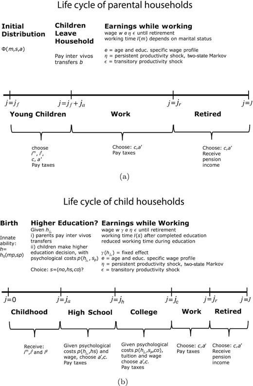
Life Cycle of Child and Parental Households.
Agents are heterogeneous with respect to the generation they belong to, |$k \in \lbrace ch,pa\rbrace ,$| either being part of the child (|$ch$|) or parental (|$pa$|) generation, and they differ by their marital status |$m \in \lbrace si,ma\rbrace$| for single (|$si$|) and married (|$ma$|), their age |$j \in \lbrace 0,\ldots ,J\lt \infty \rbrace$|, their asset position |$a$|, their current human capital |$h$|, their education level |$s \in \lbrace { {no}, {hs}, {co}}\rbrace$| for no (|${ {no}}$|) higher education (no high-school completion), high-school (|$hs$|) attendance and completion, college (|${ {co}}$|) attendance and completion, and idiosyncratic productivity risk modelled as a two-state Markov process with state vector |$\eta \in \lbrace \eta _l,\eta _h\rbrace$|, where |$\eta _l$| is low and |$\eta _h$| is high labour productivity, and transition matrix |$\pi (\eta ^\prime \mid \eta )$| and a transitory shock |$\varepsilon \in \lbrace \varepsilon _1,\ldots ,\varepsilon _n\rbrace$|. The individual state variables and the range of values they can take are summarised in Table 1.
State Variables.
| State variable | Values | Interpretation |
|---|---|---|
| |$k$| | |$k\in \lbrace ch,pa\rbrace$| | Generation |
| |$m$| | |$m\in \lbrace si,ma\rbrace$| | Marital status |
| |$j$| | |$j\in \lbrace 0,1,\ldots ,J\rbrace$| | Model age |
| |$a$| | |$a\ge -\underline{a}(j,s,k)$| | Assets |
| |$h$| | |$h\gt 0$| | Human capital |
| |$s$| | |$s \in \lbrace no,hs,co\rbrace $| | Education |
| |$\eta$| | |$\eta \in \lbrace \eta _l,\eta _h\rbrace $| | Persistent productivity shock |
| |$\varepsilon$| | |$\varepsilon \in \lbrace \varepsilon _1,\ldots ,\varepsilon _n\rbrace $| | Transitory productivity shock |
Notes: List of state variables of the economic model.
We assume that parents give birth to children at the age of |$j_{f}$| and denote the fertility rate of households by |$\xi (m,s)$|, which differs by marital status and education groups. Note that |$\xi (m,s)$| is also the number of children per household. There is no survival risk and all households live until age |$J$| and thus the cohort size within each generation is constant (and normalised to 1). We now describe in detail how life unfolds for parents, and then for children, as summarised in Figure 1.
1.1.1. Life of the parental generation
Parental households become economically active at age |$j_f$| just before their children are born. They start their economic life in marital status |$m$| and with education level |$s$|, initial idiosyncratic productivity states |$\eta$| and |$\varepsilon$| and initial assets |$a$|. These initial states are exogenously given to the household, and drawn from the population distribution |$\Phi (s,m,\eta ,\varepsilon ,a)$| that will be informed directly by the data.
Parents then observe the innate ability (initial human capital) |$h=h_{0}(s,m)$| of their children that depends on parental education |$s$| and marital status |$m$|. Children live with their parents until age |$j_a$| (parental age |$(j_{f}+j_{a})$|), at which point they leave the parental household to form their own household.
When children leave the household at parental age |$j_f+j_a$|, parents may transfer additional monetary resources as inter vivos transfers |$b$| to their children. After this transfer parents and children separate and there are no further interactions between the two generations.
Parents work until retirement at age |$j_r$|, when they receive earnings-history-dependent per-period retirement benefits |$b^p \gt 0$| and live until age |$J$|. In addition to making human capital investment decisions for their children when these are present in the household, parents in each period make a standard consumption-saving choice, where household asset choices are subject to a potentially binding borrowing constraint |$a^\prime \ge -\underline{a}(j,s,m,pa)$|, which will be parameterised such that the model replicates well household debt at the age at which households have children |$j_f.$| The borrowing limit is assumed to decline linearly to zero over the life cycle towards the last period of work at age |$j_r-1$|. Table 2 summarises the choices of parents (and children, as described in the next subsection).
Per-Period Decision Variables.
| State variable | Values | Decision period | Interpretation |
|---|---|---|---|
| |$c$| | |$c \gt 0$| | |$j\ge j_a$| | Consumption |
| |$a^{\prime }$| | |$a^\prime \ge -\underline{a}(j,s,k)$| | |$j\ge j_a$| | Asset accumulation |
| |$i^t$| | |$i^t \ge 0$| | |$j \in \lbrace j_f,\ldots ,j_f+j_a\rbrace$| | Time investments |
| |$i^m$| | |$i^m \ge 0$| | |$j \in \lbrace j_f,\ldots ,j_f+j_a\rbrace$| | Monetary investments |
| |$b$| | |$b \ge 0$| | |$j =j_f+j_a$| | Monetary inter vivos transfer |
| |$s$| | |$s \in \lbrace no,hi,co\rbrace $| | |$j=j_a$| | (Higher) education |
Notes: List of decision variables of the economic model.
1.1.2. Life of the children generation
Children are born at age |$j=0$|, but for the first |$j_{a}-1$| periods of their life do not make economic decisions. Their human capital during these periods evolves as the outcome of parental investment decisions |$(i^m,i^t)$| described above and governmental schooling input |$(i^g)$|. At the beginning of age |$j_{a},$| and based on both the level of human capital as well as the financial transfer |$b$| from their parents (which determines their initial wealth |$a$|), children make a discrete higher education decision |$s \in \lbrace { {no}, {hs}, {co}}\rbrace$|, where |$s={ {no}}$| stands in for the choice not to complete high school, |$hs$| for high-school completion and |${ {co}}$| for college completion. For simplicity, children are stand-in bachelor households through their entire life cycle.
Acquiring a high-school or college degree comes at a utility (or psychological) cost |$p(s,s_p,h)$|, which is decreasing in the child’s acquired human capital |$h$| and also depends on parental education |$s_p$|. In addition, college (|${ {co}}$|) education requires a monetary cost |$\iota \ge 0$|. Children may finance some of their college expenses by borrowing, subject to a credit limit given by |$-\underline{a}(j,s,ch)$|, which is zero for |$s \in \lbrace no,hs\rbrace ,$| i.e., for individuals not going to college. As was the case for parents, this limit decreases linearly with age and converges to zero at the age of retirement |$j_r,$| requiring the children generation to pay off their student loans prior to their retirement.
Youngsters who decide not to complete high school, |$s =no,$| enter the labour market immediately at age |$j_w(s={ {no}})=j_{a}$|. Those who decide to complete high school, but not to attend college, do so at age |$j_w(s=hs)=j_h\gt j_a$|. While at high school, |$\lbrace j_a,\ldots ,j_h-1\rbrace$|, they work part time at wages of education group |$s={ {no}}$|. Youngsters who decide to attend college enter the labour market at |$j_w(s=co)=j_{c}$| and also work part time at wages of education group |$s={ {no}}$| during their high-school and college years |$\lbrace j_a,j_c-1\rbrace .$|
1.2. Decision Problems
Since we focus on a single parent and children generation, we can solve the model backward, starting from the dynamic programming problem of the children.
1.2.1. Children
The first meaningful economic decision in the children generation takes place at age |$j_a$|, when children leave the parental household with the receipt of inter vivos transfers, which constitute initial assets |$a,$| as well as with human capital |$h$|.
The retirement phase. During retirement, at ages |$\lbrace j_r,\ldots ,J\rbrace$|, all three education groups of the children generation solve a standard consumption-saving problem given in Online Appendix A.1.
1.2.2. Parents
1.3. Government
The government runs a pension system with a balanced budget. It also finances exogenous government spending, expressed as a share of aggregate output |$G/Y$|, and aggregate education subsidies (of pre-tertiary and tertiary education) through consumption taxes, capital income taxes and a progressive labour income tax code. In the initial scenario without the COVID-19 shock, the government budget clears by adjustment of the average labour income tax rate. In the thought experiments we hold all tax parameters constant, therefore implicitly assuming that the shortfalls or surpluses generated by a change in the environment are absorbed by government debt serviced by future generations.
1.4. Thought Experiment
We compute an initial stationary partial equilibrium with exogenous wages and returns prior to model period |$t=0$|. In period |$t=0$|, the COVID-19 shock unexpectedly occurs, and from that point on unfolds deterministically. That is, factor prices and fiscal policies are fixed, and households get surprised once by the shock, after which they have perfect foresight with respect to aggregate economic conditions. The COVID-19 school closures are represented in the model by a temporary (one year) reduction in public investment |$i^g$| into child human capital production.
We then trace out the impact of this temporary shock on parental human capital inputs (both time and money) and intergenerational transfer decisions, as well as on the education choices, future labour market outcomes and welfare of the children generation, both in terms of its aggregates as well as in terms of its distribution. Since children differ by age at the time of the shock (as well as in terms of parental characteristics), so will the long-run impact on educational attainment, future wages and welfare. We place special emphasis on this heterogeneity.
2. Calibration
A subset of parameters is calibrated exogenously outside the model, summarised in Table 3. The subset of second-stage parameters, summarised in Table 4, is calibrated endogenously by matching moments in the data. In the calibration, we use data from the PSID, including its Child Development Supplement (CDS),6 and the NLSY79.7 We now describe in detail our choice of first-stage parameters and the moments we match to calibrate the second-stage parameters.
First-Stage Calibration Parameters.
| Parameter | Interpretation | Value | Source (data/literature) |
|---|---|---|---|
| Population | |||
| |$j=0$| | Age at economic birth (age four) | 0 | |
| |$j_{a}$| | Age at beginning of economic life (age sixteen) | 6 | |
| |$j_{h}$| | Age at finishing HS (age eighteen) | 7 | |
| |$j_{c}$| | Age at finishing CL (age twenty-two) | 9 | |
| |$j_{f}$| | Fertility age (age thirty-two) | 14 | |
| |$j_{r}$| | Retirement age (age sixty-six) | 31 | |
| |$J$| | Max. lifetime (age eighty) | 38 | |
| |$\xi (m,s)$| | Fertility rates | See main text | PSID 2011–17 |
| |$\Phi (j_f,m,s)$| | Distribution of parents by martial status and education, age |$j_f$| | See main text | PSID 2011–17 |
| Preferences | |||
| |$\theta$| | Relative risk aversion parameter | 1 | |
| |$\varphi$| | Curvature of labour disutility | 0.5 | |
| Labour productivity | |||
| |$\lbrace \epsilon (j,s,m)\rbrace$| | Age profile | See main text | PSID 1968–2012 |
| |$[\varepsilon _l,\varepsilon _h]$| | Realisations of transitory shock | |$[0.881, 1.119]$| | PSID 1968–2012 |
| |$[\eta _l,\eta _h]$| | States of Markov process | [0.8226, 1.1774] | PSID 1968–2012 |
| |$\pi _{hl}$| | Transition probability of Markov process | 0.0431 | PSID 1968–2012 |
| |$\pi ^{r}_{hl}(s)$| | Transition probability of Markov process after lockdown | [0.0493,0.0486,0.0456] | See main text |
| |$\pi ^{r}_{ll}(s)$| | Transition probability of Markov process after lockdown | [0.9630,0.9624,0.9594] | See main text |
| |$\chi ^s$| | Hours worked for students, as a fraction of full time (HS and CL) | |$\lbrace 0.2,0.5 \rbrace $| | See main text |
| |$\gamma (s,h)$| | Ability gradient of earnings | See main text | NLSY79 |
| Endowments | |||
| |$r$| | (Annual) interest rate | 4.0% | Siegel (2002) |
| |$l(m)$| | Average hours worked by marital status (annual) | |$\lbrace 1868, 3810\rbrace $| | PSID 2011–17 |
| |$\Phi (a|j_f,m,s)$| | Asset distribution of parents by martial status and education, age |$j_f$| | See main text | PSID 2011–17 |
| |$\underline {a}(j_f,m, s,pa)$| | Borrowing limit for parents at age |$j_f$| | See main text | PSID 2011–17 |
| |$rp(m=si, s, pa)$| | Education-specific repayment amount for parents: singles | See Subsection 2.4 | |$\lbrace 0.006, 0.083, 0.151 \rbrace$| |
| |$rp(m=ma, s, pa)$| | Education-specific repayment amount for parents: couples | See Subsection 2.4 | |$\lbrace 0.048, 0.129, 0.110 \rbrace$| |
| Ability/human capital and education | |||
| |$\iota$| | College tuition costs (annual, net of grants and subsidies) | $14,756 | Krueger and Ludwig (2016) |
| |$\underline {a}(j \in [j_h,j_c-1],{ {co}},ch)$| | College borrowing limit | $45,000 | Krueger and Ludwig (2016) |
| |$rp(ch)$| | Repayment amount for children who choose college | 0.049 | See Subsection 2.7 |
| |$\sigma ^{h}$| | Elasticity of subst. between human capital and CES invest. aggregate | 1 | Cunha et al. (2010) |
| |$\sigma ^{g}$| | Elasticity of subst. between public invest. and CES aggregate of private invest. | 2.43 | Kotera and Seshadri (2017) |
| |$\sigma ^{m}$| | Elasticity of subst. between monetary and time investments | 1 | Lee and Seshadri (2019) |
| |$\kappa ^m_3$| | CES share parameter of monetary and time investments (age bin 6–8) | 0.5 | Normalisation |
| |$\kappa ^g_j=\bar{\kappa }^g,j\gt 0$| | Share of government input for ages six and older | 0.676 | Kotera and Seshadri (2017) |
| |$\Phi (h(j=0)|s_p,y_p,a_p)$| | Innate ability distribution of children by parental characteristics | See main text | PSID CDS I |
| |$\underline{h}_0$| | Normalisation parameter of initial distribution of initial ability | 0.1248 | PSID CDS I–III |
| Government policy | |||
| |$\xi$| | Public CL education subsidy | 38.8% | Krueger and Ludwig (2016) |
| |$i^g_j$| | Public early education spending by age | |$\approx \$\text{5,000}$| | UNESCO (1999–2005) |
| |$\tau _c$| | Consumption tax rate | 5.0% | Legislation |
| |$\tilde{\tau }_k$| | Capital income tax rate | 20% | Legislation |
| |$\tau ^p$| | Social security payroll tax | 12.4% | Legislation |
| |$G/Y$| | Government consumption to GDP | 13.8% | Current value |
Notes: First-stage parameters calibrated exogenously by reference to other studies and data.
Second-Stage Calibration Parameters.
| Parameter | Interpretation | Value |
|---|---|---|
| Preferences | ||
| |$\beta$| | Time discount rate (target: asset to income ratio, ages 25–60) | 0.9808 |
| |$\nu$| | Altruism parameter (target: average IVT per child) | 0.8380 |
| Labour productivity | ||
| |$\rho _0(s)$| | Normalisation parameter (target: |$ \mathbb {E} \gamma (s,h)=1$|) | |$[0.1890, 0.0034, -0.2015]$| |
| Human capital and education | ||
| |$\kappa$| | Utility weight on time invest. (target: average time invest.) | 0.7310 |
| |$\kappa ^h_j$| | Share of human capital (target: average monetary & slope of time investments) | cf. Online Appendix Figure B1 |
| |$\kappa ^m_j$| | Share of monetary input (target: slope of monetary invest.) | cf. Online Appendix Figure B1 |
| |$\kappa ^g_0$| | Share of government input for age bin 4–6 (target: average time invest. age bin 4–6) | 0.4437 |
| |$\bar{A}$| | Investment scale parameter (target: average HK at age |$j_a$|) | 1.1989 |
| |$\tilde{A}$| | Investment scale parameter in HS (target: average HK at age |$j_{a+1}$|) | 1.0739 |
| |$\phi$| | Utility costs |$s=hs$| (target: fraction of group |$s=hs$|) | 0.0561 |
| |$\tilde{\varrho }(s^p=no)=\tilde{\varrho }(s^p=hs)$| | Utility costs |$s={ {co}}, s^p=no \wedge s^p=hs$| (target: fraction of group |$s=co$|) | 1.2120 |
| |$\tilde{\varrho }(s^p=co)$| | Utility costs |$s={ {co}}, s^p=co$| (target: conditional fraction of group |$s=co$|) | 0.1707 |
| Government policy | ||
| |$\lambda$| | Level parameter of HSV tax function (balance government budget) | 0.8880 |
| |$\rho ^p$| | Pension replacement rate (balance social security budget) | 0.1893 |
Notes: Second-stage parameters calibrated endogenously by targeting selected data moments.
2.1. Age Brackets
The model is calibrated at a biannual frequency. We initialise the parental economic life cycle when their children are of age four, model age |$j=0$|. The reason for this initialisation age is the calibration of the initial human capital endowment |$h(j=0)$|, which is informed by data on test score measures at child biological ages three to five. Thus, children are irrelevant to the economic model for the first three years of their biological lives. Parental age at the economic ‘birth’ of children is |$j_f=14$|, which we also refer to as ‘fertility’ age. This corresponds to a biological age of thirty-two, when children are of biological age four.8 Children make the higher eduction decisions at biological age sixteen, model age |$j_a=6$|. Children who complete high school stay in school for one additional model period; thus, high school is completed at |$j_h=7$|. Children who attend college stay in college for two model periods; thus, college is completed at |$j_c=9$|. Retirement is at exogenous age |$j_r=31$|, corresponding to biological age sixty-six. Households live at most with certainty until age |$J=38$|, biological age eighty.
2.2. Prices and Income Process
We normalise wages to |$w=1$| and set the interest rate to an annual rate of |$4\%$| based on Siegel (2002). The calibration of the stochastic wage process based on PSID data involves a standard calibration of the temporary and permanent shock distributions based on GMM estimates, described in detail in Online Appendix Section B.2.
2.3. Preferences
When children live in the parental household, we have |$x={[\ell (m)+ \kappa \cdot \xi (m,s) \cdot i^t ]}/{(1+\mathbf {1}_{m=ma} )}$|. Here |$\ell (m)$| is the hours worked by marital status, which we estimate from the data, giving annual hours of |$\ell ({ {si}})=1868$| and |$\ell (ma)=3810$|. The time cost parameter |$\kappa$| is calibrated to match average time investments by parents into the education of children, giving |$\kappa =0.74$|.
We calibrate the parameters of the cost function to match education shares in the data for the three groups |$s \in \lbrace { {no}, {hs}, {co}}\rbrace$|. We measure these shares for adults older than age twenty-two—which is the labour market entry age of all education groups in the model—and younger than age thirty-eight based on the PSID waves 2011, 2013, 2015 and 2017.9 Parameter |$\phi$| is calibrated to match the fraction of children without a high-school degree of 12.16%, giving |$\phi =0.06$|. With regard to the additional utility costs during the college period we restrict |$\tilde{\varrho }(no)=\tilde{\varrho }(hs)$| and calibrate it to match the fraction of children with a college degree of 33.21%, giving |$\tilde{\varrho }(no)=\tilde{\varrho }(hs)=1.21$|. Finally, parameter |$\tilde{\varrho }(s^p=co)$| is calibrated to match the fraction of children in college conditional on parents having a college degree of 63.3%, cf. Krueger and Ludwig (2016), giving |$\tilde{\varrho }(co)=0.17$|.
Households discount utility at rate |$\beta$|. We follow Busch and Ludwig (2020) and calibrate it to match the assets to income ratio in the PSID for ages twenty-five to sixty, giving |$\beta =0.98$| annually.
Utility of future generations is additionally discounted at rate |$\nu$|, chosen so that the average per-child inter vivos transfer is $61,200, as implied by the Rosters and Transfers supplement to the PSID,10 giving |$\nu =0.84$|.
2.4. Initial Distribution of Parents
For the initial distributions of parents at the fertility age, we restrict the sample to parents aged 25–35, leaving us with 3,024 observations.11
Marital status. Marital status is measured by the legal status of parents. This gives a share of singles of |$52\%$| and a share of married households of |$48\%$|.
Education categories. We group the data by years of education of household heads older than age twenty-two. Less than high school, |$s={ {no}}$|, is for less than twelve years of formal education. High-school completion (but no college) is for more than twelve but less than sixteen years of education. College is at least sixteen years of education. The population shares of parents in the three education categories by their marital status are summarised in columns 2 and 3 of Table 5.12
Household Shares and Characteristics by Education and Marital Status.
| % fraction of households | No. of children | Lower asset limit | ||||
|---|---|---|---|---|---|---|
| Education |$s$|/marital status |$m$| | |$si$| | |$ma$| | |$si$| | |$ma$| | |$si$| | |$ma$| |
| |${ {no}}$| | 0.2194 | 0.1621 | 2.36 | 2.33 | −2,380 | −18,931 |
| |$hs$| | 0.6064 | 0.5577 | 1.86 | 2.15 | −33,065 | −51,332 |
| |${ {co}}$| | 0.1742 | 0.2802 | 1.77 | 1.96 | −60,037 | −43,629 |
Notes: Columns 2 and 3 show fractions with education |$s \in \lbrace { {no}, {hs}, {co}}\rbrace$| by marital status. Columns 4 and 5 show numbers of children, and columns 6 and 7 lower asset limits for parents at model age |$j_f$|, expressed in 2010 dollars, by marital status and education.
Demographics. The number of children by marital status and education of parents |$\xi (m,s)$| is computed as the average number of children living in households with household heads aged 25–35; cf. columns 4 and 5 of Table 5.
2.5. Acquired Human Capital and Earnings
2.6. Human Capital Production Function
Initial human capital. For calibration of the distribution of initial human capital |$h_0(s_p,m_p)$|, we recur to the Letter Word test score distribution in the PSID CDS surveys I–III, and match it to parental characteristics by merging the survey waves with the PSID.
Online Appendix Table B3 reports the joint distribution of average test scores of the children by parental education and marital status. We base the calibration of the initial ability distribution of children on this data by drawing six different types of children depending on the combination of marital status and parental education.15 Children’s initial human capital is normalised as the test score of that |$m^p,s^p$|-group relative to the average test score. We further scale the resulting number by the calibration parameter |$\bar{h}_0$| and, thus, initial human capital of the children is a multiple of |$\bar{h}_0$|. Parameter |$\bar{h}_0$| is calibrated exogenously to match the ratio of mean test scores at ages 3–5 to mean test scores at ages 16–17, which gives |$\bar{h}_0=0.125$|. Initial abilities relative to average abilities and the corresponding multiples of |$\bar{h}_0$| for the six types are contained in Table B3 of Online Appendix B.
In the second nest, we set the substitution elasticity |$\sigma ^g$| between private and government investments to |$\sigma ^g = 2.43$|, estimated by Kotera and Seshadri (2017)—who estimated the parameters of a CES nesting of private and public education investments similar to ours based on US data. Thus, parental and government investments are gross substitutes, but substitution across these education inputs is far from perfect. Since this elasticity of substitution is a crucial parameter, we show sensitivity of the results with respect to it in Section 5. We restrict |$\kappa ^g_j=\bar{\kappa }^g$| for |$j \gt 0$| and calibrate it exogenously again according to the estimates by Kotera and Seshadri (2017), giving |$\bar{\kappa }^g=0.676$|. At biological age four of the child, children are still in kindergarten, and we separately calibrate |$\kappa ^g_{0}$| to match the average time investments by parents into their children at that age. This gives |$\kappa ^g_0 = 0.44$|. By |$\bar{A}$| we denote a computational normalisation parameter that we choose such that average acquired human capital is equal to 1, sufficiently below the maximum human capital gridpoint, giving |$\bar{A}=1.20$|.
2.7. College Tuition Costs and Borrowing Constraint of Children
2.8. Government
The government side features the budget of the general tax and transfer system and a separate budget of the pension system, all set to mimic the US system. In the general budget the revenue side is represented by consumption, capital income and progressive labour income taxes. Details of the calibration are given in Online Appendix Section B.5.
Exogenous government spending (net of spending on education) is set to |$G/Y \%= 13.8\%$|. In addition, the government spends on schooling for children and pays the college subsidy for college students. The former we approximate as $5,000 per pupil based on UNESCO (1999–2005) data, as for example in Holter (2015). The latter is set to |$38.8\%$| of average gross tuition costs, as in Krueger and Ludwig (2016). Assuming, as in Krueger and Ludwig (2016), that the difference between net and gross tuition costs is due to both a public and a private subsidy with the latter not being explicitly modelled in our setup19 gives an average public subsidy of |$\$ 6,119$| per student.
2.9. Evaluating Non-Targeted Predictions of the Model
2.9.1. Time and resource investments
Figure 2 shows average time and monetary investments in the model and the data by child age. The good match of the model of time investments in panel (b) is a consequence of calibration since this is a targeted profile through age-dependent parameter |$\kappa ^h_j$| and parameter |$\kappa ^g_0$|. Monetary investments in panel (a) are slightly downward sloping in the data, and we match the lower slope of monetary investments compared to time investments through the age dependency of |$\kappa ^m_j$|.
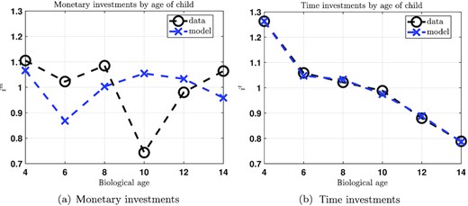
Monetary and Time Investments by Age of Child.
Notes: Average monetary and time investments by children’s biological age in the data (black circles) and model (blue crosses).
Figure 3 shows the analogous output by parental education levels, all of which are not targeted in the calibration. The model matches well the positive slope of both types of investment in parental education. Since income and initial wealth of a household is increasing in the household’s education, it is perhaps not surprising that more highly educated parents invest significantly more resources in each child, especially since these households have fewer children. The same observation (number of children decreasing in household education) is also responsible for the mildly increasing per-child time investment by parental education (see Figure 3(b)).
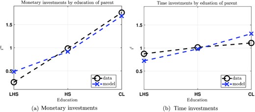
Monetary and Time Investments by Education of Parents.
Notes: Average monetary and time investments by parents’ education in the data (black circles) and model (blue crosses). LHS, less than high school (|$s={ {no}}$|); HS, high school (|$s=hs$|); CL, college (|$s=co$|).
2.9.2. Intergenerational persistence in education
In our calibration we also do not target directly any measure of intergenerational persistence in education. We measure this persistence by the regression coefficient |$\beta _1$| in a regression of the education of a child on parental education, |$s = \beta _0 + \beta _1 s^p + \epsilon$|. In this regression we form two groups, non-college for |$s \in \lbrace no,hs\rbrace$| and |$s^p \in \lbrace no,hs\rbrace$|, and college for |$s=co$| and |$s^p=co$|. Standard estimates of intergenerational education persistence according to this metric range from 0.4 to 0.5 and our (non-targeted) coefficient estimate of |$\beta _1=0.47$| is in that range.20
2.9.3. Evidence on the long-run earnings impact of school closures
Our model implies a significant decline of incomes for children affected by the closure of schools. We are not aware of any empirical evidence on the effects of school closures on long-run outcomes of children in the United States and therefore resort to the reduced-form evidence of Jaume and Willén (2019) on the effects of teacher strikes in Argentina between 1983 and 2014 on long-run economic outcomes of the affected children. Their main estimates refer to the closing of primary schools by half a year, and they report that this leads to a reduction of wages at ages 30–40 by about |$2\%\!{-}\!3\%$|. In our model, we consider for our main experiment an exogenous reduction of investments by the government corresponding to a school closure by a year, but in a sensitivity analysis also report results for half year school closures. In that experiment our model predicts an average wage loss at biological ages 30–40 for children who were of biological age six in the period of the lockdown of −1.21%, which is around one-half the size of the estimates from Jaume and Willén (2019), for a different country in a different time period.
2.9.4. Time investment into children during the COVID-19 crisis
Finally, our calibration implies that the time investment response of parents in our full experiment—where government education investments |$i^g$| are reduced and where parental households are both subject to a negative productivity shock and a negative hours worked shock calibrated as described above—translates to 1.17 hours per day of increased time investments into children during the period of the lockdown of schools.21 This lies well in the range of estimates provided on the basis of real-time surveys by Adams-Prassl et al. (2020).
3. Aggregate Consequences of the School Closures
In this section, we start out analysing the average consequences of the school closures for human capital accumulation, educational attainment, earnings and ultimately welfare of children. We then describe the optimal parental reactions, analyse their importance in counteracting the negative effects of the school closures and their welfare effects for the parents.
3.1. Human Capital Losses, Educational Attainment and Earnings
The lockdown of schools leads to a decline in educational attainment when the children affected by the COVID crisis today make their tertiary education decisions at age sixteen. As Table 6 (second column) shows, across all age cohorts the share of children that will end up dropping out of high school (i.e., choosing |$s={ {no}}$|) increases by 1.92 percentage points, and the share of college-educated children will decline by |$-2.34$| percentage points. While these shifts do not appear to be dramatic, they correspond to a |$16\%$| increase in the share of children without high-school degrees, and a |$-7\%$| decrease in the share of college-educated children.
Aggregate Outcomes for Main Experiments.
| Baseline | Change for children of biological age | |||||||
|---|---|---|---|---|---|---|---|---|
| Average | 4 | 6 | 8 | 10 | 12 | 14 | ||
| Change in percentage points | ||||||||
| Share |$s={ {no}}$| | 12.07 | 1.92 | 1.66 | 3.08 | 2.40 | 1.85 | 1.44 | 1.12 |
| Share |$s=hs$| | 54.64 | 0.41 | 0.10 | −0.13 | 0.35 | 0.63 | 0.76 | 0.78 |
| Share |$s=co$| | 33.30 | −2.34 | −1.75 | −2.95 | −2.74 | −2.49 | −2.20 | −1.89 |
| Change in percentages | ||||||||
| Average HK | 1.00 | −3.32 | −2.92 | −4.34 | −3.85 | −3.38 | −2.92 | −2.48 |
| PDV gross earn | $846,473 | −2.10 | −1.82 | −2.73 | −2.44 | −2.15 | −1.87 | −1.59 |
| PDV net earn | $696,076 | −1.68 | −1.45 | −2.20 | −1.96 | −1.72 | −1.49 | −1.26 |
| Child CEV | 0.00 | −1.21% | −1.09% | −1.57% | −1.40% | −1.23% | −1.07% | −0.91% |
Notes: Share |$s \in \lbrace { {no}, {hs}, {co}}\rbrace$|, the education share in each respective education category where |$s={ {no}}$| denotes less than high school, |$s=hs$| denotes high school and |$s=co$| denotes college. Average HK, the average acquired human capital at age sixteen; PDV gross earn, the present discounted value of gross earnings assuming labour market entry at age twenty-two and retirement at age sixty-six; PDV net earn, present discounted value of net earnings; CEV, consumption equivalent variation. Columns for biological ages 4–14 show the respective percentage point changes of education shares, the percentage changes of acquired human capital and average earnings, and the CEV expressed as a percentage change, for children at various ages at the time of the school closures. Column ‘Average’ gives the respective average response. The CEV is the consumption equivalent variation of welfare measure (5).
The reason for the reallocation towards lower final educational attainment is the reduction in the amount of human capital the average child arrives with at age sixteen, which falls by |$-3.3\%$|. As Table 7, first column, demonstrates, in response to the COVID-19 school closures, parents increase their private investments into children, both in terms of resources as well as in terms of time. However, as discussed in greater detail below, this reaction is not sufficient to fully compensate the loss of government inputs into human capital production in the form of schooling. Consequently, average human capital at age sixteen is lower than without the COVID-19 school closure shock, and the children affected by the shock choose on average lower educational attainment. The lower educational attainment together with the lower human capital in turn imply losses in the average discounted value of gross lifetime earnings by |$-2.1\%$|; see the fifth row of Table 6. Thus, a transitory shock of closed schools for one year alone leads to a permanent reduction in long-term earnings by more than 2% for the affected children, on average, even after taking optimal parental adjustments into account. In terms of present discounted dollars, this corresponds to an average per-person loss of $17,776 dollars in year 2019 prices.
Parental Decisions.
| Baseline | % change for children of biological age | |||||||
|---|---|---|---|---|---|---|---|---|
| Average | 4 | 6 | 8 | 10 | 12 | 14 | ||
| Panel A: in the period of school closures | ||||||||
| Average monetary invest. | $1,385 | 35.44 | 23.73 | 38.08 | 36.72 | 36.77 | 37.82 | 39.51 |
| Average time invest. | 25.17 | 16.62 | 10.78 | 17.40 | 16.90 | 17.17 | 18.04 | 19.44 |
| Panel B: averages over remaining childhood | ||||||||
| Average monetary invest. | $1,381 | 14.06 | 2.90 | 5.37 | 7.49 | 11.01 | 18.08 | 39.51 |
| Average time invest. | 22.56 | 6.73 | 1.31 | 2.37 | 3.44 | 5.16 | 8.64 | 19.44 |
| Average IVT | $61,255 | 0.73 | 0.43 | 1.79 | 1.11 | 0.64 | 0.31 | 0.11 |
Notes: In panel A we present columns for biological ages 4–14 that show the percentage changes in monetary investments and time investments in the period of the school closures. In panel B we present columns for biological ages 4–14 that show the percentage changes in monetary investments, time investments and inter vivos transfers for children at various ages at the time of the school closures. For monetary and time investments, these are averages of the percentage changes of the respective investment over the remaining life cycle, so, e.g., for a child of age six, the percentage change is the average of the percentage changes of investments at ages 6–14 for this child. Column ‘Average’ is the raw average across the biological ages of children.
In order to get a better sense of the magnitude of the future earnings declines, we now discount the present discounted gross earnings losses reported in row five of the table, which the children will experience at age twenty-two, to today and aggregate them across all children, using the number of children in the current US population taken from the Human Mortality Database. Relating the resulting aggregate loss to the 2019 US GDP of |$\$21.43$| trillion shows that these future earnings losses are equivalent to a loss of |$-3.0\%$| of 2019 US GDP. Thus, the aggregate indirect economic costs caused by the school closures are quite sizeable. The percentage loss in net earnings (after taxes and transfers) is lower (|$-1.68\%$|; see the sixth row of Table 6). This is due to the progressive labour income tax schedule, which implies that a reduction of gross earnings on average leads to a reduction of tax payments (or an increase in transfers); the mirror image is of course a corresponding reduction in tax receipts by the government.
The remaining columns of Table 6 show that there is considerable heterogeneity in the size of these effects by the age of the child at the time the schooling shock hits.22 Overall, the most severely affected age group are the six-year-old children, i.e., those at the start of primary school. For them, the predicted share of high-school dropouts increases by 3.08 percentage points, the share of college-educated decreases by |$-2.95$| percentage points and their average long-term gross earnings drop by |$-2.73\%$|, which corresponds to a present discounted earnings loss of $23,109. Younger children are most affected by the school closures due to the self-productivity and the dynamic complementarity implied by the human capital production function: a decrease in human capital accumulation at younger ages due to the school closures translates into lower human capital and lower optimal parental investment in human capital in the future, as we discuss in greater detail in Subsection 3.3.
Even though the adverse effect of school closures on human capital accumulation and future educational attainment is most severe for young school children, it is non-negligible even for the cohort of fourteen-year-old children when the COVID crisis hits. For this age cohort, the predicted share of high-school dropouts increases by 1.12 percentage points, the share of college-educated decreases by |$-1.89$| percentage points and the present discounted value of their average gross earnings during the rest of life falls by |$-1.59\%$|; see the last column of Table 6. Note that compared to age six-year-old children, children of age four are more shielded against the negative effect of experiencing closures of day care centres and kindergarten, due to the lower importance of governmental inputs relative to parental inputs in the human capital production function at that age.23
3.2. The Welfare Cost of School Closures on Children
There are three dimensions along which the cross-sectional distribution for a given cohort deteriorates due to the COVID-19 schooling shock. First, children reach a different human capital position |$h$| at age |$j_a$| when they split off from the parental household; second, they receive different amounts of inter vivos transfers from their parents and thus start their working lives with different assets; and third, they make different tertiary education decisions and thus start working life at age |$j_c$| with a different education distribution.
To quantify the welfare consequences of the school closures, we compute, for each child cohort |$j$|, the consumption equivalent variation (CEV) of the COVID-19 schooling shock. That is, we calculate the uniform percentage increase in consumption such that the average labour market entrant of a cohort of age |$j$| is indifferent between the welfare consequences arising from the original cross-sectional distribution across states at labour market entry and its COVID-impacted counterpart. As the last row of Table 6 shows, the welfare losses from the closing of schools are quite substantial, with a reduction of welfare as measured by the CEV of |$-1.21\%$| on average. Thus, the temporary year-long lockdown of schools has strong long-run welfare consequences for children, worth in the order of |$-1.21\%$| of permanent consumption, and this despite the increased human capital investments by parents through home schooling, increased resource investments and increased inter vivos transfers. For the least affected cohorts, children aged fourteen at the time of school closures, the welfare losses are still |$-0.91\%$|, and for the most affected cohort, children of age six, welfare losses amount to |$-1.57\%$| of consumption. We view these as substantial welfare losses, considering that the school closures are purely temporary shocks, and parents adjust their behaviour optimally to counteract the adverse effects on their offspring.
3.3. Parental Responses to School Closures
The previous section painted a fairly dire picture of the long-run outcomes of children impacted by COVID-19-induced school closures. We now document that these effects emerge despite substantial efforts of parents to take mitigating actions. In our model, parents have three principal means by which they can cushion the blow to their children of the COVID-19-induced schooling crisis. They can expand their time investments and their resource investments into the children’s human capital accumulation during the schooling ages, and they can facilitate attending high school and college by providing children with inter vivos transfers. Table 7 shows that they do all three. For a given age column |$j \in \lbrace 4,6,\ldots ,14\rbrace$|, panel A of Table 7 gives the percent change of investments during the impact period, relative to the pre-COVID-19 scenario. The second column displays the unweighted average, across all children ages, of the age-specific percent changes. Panel B shows the average change across the remaining child years, and therefore takes a longer-term perspective. For example, for children aged four during the crisis, panel B shows the average change in parental investments from ages 4–14, while for children aged fourteen during the school closure, it captures the change in parental investments only at this age (since it is the last age that the child spends in the household).
On average, parents on impact increase their monetary investments into their children’s education by |$35.44\%$|, their time investment by |$16.6\%$|—which corresponds to about one additional hour per-child per day (see footnote 23 for the relevant transformation)—and their inter vivos transfers to children, once these children leave the household, by |$0.73\%$|. Thus, overall, parents respond to the school closures with positive and substantial additional investments into their children in all three dimensions, albeit significantly stronger with their direct human capital investments than with their inter vivos transfers.
As the remaining columns of the table demonstrate, the exact composition of the parental adjustment depends on the age of the child, but is consistently stronger for resource investments (albeit starting from a fairly low level of $1,385 per-year per child) than time investment and eventual inter vivos transfers. Monetary and time parental investments increase the least for four-year-old children, and the most for fourteen-year-old children, with a fairly flat profile between ages six and fourteen. Note that these changes happen against the backdrop of higher pre-COVID investments (especially time investments; see the upper left panel of Figure 4) for younger children. In absolute terms, changes in time investments are decreasing in the age of the child starting at age six, but changes in monetary investments are increasing.
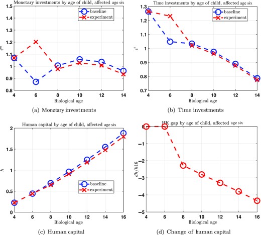
Monetary and Time Investments and Human Capital over the Child's Remaining Life Cycle for Children Age Six.
Notes: Average investments for children age six over their (remaining) life cycle and acquired human capital at various ages. Blue circles, baseline steady state; red crosses, experiment. (a) Monetary investments; (b) time investments; (c) acquired human capital; (d) change of acquired human capital, expressed relative to baseline human capital at age sixteen. Since these are averages for children age six in the period of the lockdown, the initial points at age four for investments and at ages four and six for acquired human capital are identical in the baseline and in the experiment.
Observe that, for none of the children's ages, parents find it optimal to completely offset the effect of the public school closure on human capital investment during the period of the crisis, since this would compromise their own consumption and lifetime utility too severely. Consequently, all children leave the crisis period with less human capital than they otherwise would have had without the school closures. Because of the dynamic complementarity of human capital and investment, this reduction curbs the incentives for private parental human capital investments in all future periods. This effect is more severe the longer the human capital accumulation phase during school ages still is, that is, it impacts young children the most. Furthermore, even in the crisis period itself, as Table 7 shows, monetary and time investments increase strongest for older children in percentage terms. For time investments, part of this again comes from the fact that baseline time investment is highest for the youngest children. An additional reason lies in the decreasing importance of investment relative to own human capital in the human capital accumulation process over the child's life cycle: this necessitates stronger investment responses by parents of older children, in percentage terms, to counteract the negative effects of the school closures. Last, parents of young children have on average lower incomes and assets than parents of older children, making it more likely that they are borrowing constrained. Thus, for them, it is relatively more attractive to increase future inter vivos transfers than current resource investments into their children. This mechanism is particularly relevant for asset poor young parents, which constitute the largest fraction of borrowing constrained households in our model.
We display the dynamic adjustments of time and monetary investments into children that are six years old at the time of the school closures in Figure 4. Panels (a) and (b) depict time and monetary investments of parents of these children over their life cycle, both in the benchmark no-crisis scenario and in the presence of the school closures. Panel (c) of the same figure shows the resulting evolution of human capital as the child progresses through school ages following the COVID-19 shock, and panel (d), for better visualisation, displays the human capital stock over the life cycle, in deviation of the no-COVID benchmark (and expressed as a percentage of the age-sixteen pre-COVID human capital level). In the period of the lockdown, at biological age six, there is a substantial increase in parental investment. Private resource investments rise by 38.1% and time investment by 17.4%. This is not enough, however, to compensate for the 50% decline in government inputs during this two-year period (a year of lost schooling), and thus at biological age eight human capital is at a slightly lower level than in the no-COVID scenario.24 In response, future human capital investment incentives are dampened due to the dynamic complementarity feature of the human capital production function. Therefore, both time and especially resource investments are lower in subsequent periods (at older ages of the child), with the consequence that the child ten years after the crisis (at age sixteen) enters the tertiary education phase with less human capital, therefore opting (on average) for lower educational attainment and the associated reduction in lifetime earnings. However, the widening of the human capital gap shown in panel (d) of Figure 4 is primarily due to the self-productivity feature of the human capital production function. If in all periods after the lockdown parents were to keep their investments at the (higher) baseline level, the observed human capital gap at age sixteen would close by merely 4.6%. Thus, the main driver of the human capital loss at age sixteen for children of age six at the time of the COVID school closures is the fact that the crisis reduces human capital accumulation on impact (even when partially offset by parental investments) that makes children less effective learners as teenagers and thus results in lower human capital at the age when the tertiary education decision is being made.
In contrast to parental monetary and time investments, inter vivos transfers increase strongest for the six-year-old children, and then less for older children. Ultimately, parents care about the lifetime utility of their offspring, and not about the means by which they buffer the welfare of children against the adverse schooling shock. Given the dynamic complementarity mechanism explained above, it is relatively more efficient to support younger children more significantly through higher inter vivos transfers, whereas for older school-aged children, human capital investments are the better option to smooth the COVID schooling shock. Moreover, parents of six-year-old children at the time of school closures are more likely borrowing constrained at that point in time than when the children are sixteen.
To understand the importance of the reaction of parents to the closure of schools, we analyse the results of a model in which we hold all parental decisions constant. Thus, governmental inputs fall due to the school closures, but parental inputs remain unchanged—both investments into the human capital of their children and their inter vivos wealth transfers. Results for this experiment on aggregate effects are summarised in Table 8, which should be compared to Table 6.
Aggregate Outcomes under Constant Parental Decisions.
| Baseline | Change for children of biological age | |||||||
|---|---|---|---|---|---|---|---|---|
| Average | 4 | 6 | 8 | 10 | 12 | 14 | ||
| Change in percentage points | ||||||||
| Share |$s={ {no}}$| | 12.07% | 2.60 | 2.38 | 3.96 | 3.19 | 2.52 | 1.99 | 1.54 |
| Share |$s=hs$| | 54.64% | −0.40 | −0.88 | −1.14 | −0.57 | −0.16 | 0.09 | 0.28 |
| Share |$s=co$| | 33.30% | −2.20 | −1.50 | −2.82 | −2.62 | −2.36 | −2.08 | −1.82 |
| Change in percentages | ||||||||
| Average HK | 1.00 | −4.28 | −3.86 | −5.38 | −4.90 | −4.39 | −3.85 | −3.31 |
| PDV gross earn | $846,473 | −2.55 | −2.25 | −3.21 | −2.92 | −2.62 | −2.30 | −1.98 |
| PDV net earn | $696,076 | −2.04 | −1.80 | −2.59 | −2.35 | −2.10 | −1.84 | −1.58 |
| CEV children | − | −1.63% | −1.50% | −2.11% | −1.87% | −1.65% | −1.43% | −1.22% |
Notes: This table is the analogue to Table 6 where parental monetary and time investment decisions and inter vivos transfer decisions are held constant. This is computed by holding parental policy functions constant and by aggregating with a hypothetical distribution of children over human capital computed under constant decisions.
We observe that the aggregate effects are now larger than in the scenario of school closures and full parental behavioural adjustments. Acquired human capital of children falls now by |$4.28\%$| on average instead of |$3.32\%$| when parents react optimally. The share of high-school dropouts now increases by 2.60 percentage point instead of 1.92 percentage points when parents re-optimise their decisions. However, the share of college-educated children does not drop by more and in fact decreases by slightly less than when parents react optimally to the school closures, by |$-2.20$| instead of |$-2.34$| percentage points. The reason for a slightly lower drop of the share of college-educated children is the constancy of inter vivos transfers that induce marginal students to attend college. With re-optimising parents, inter vivos transfers would decrease for this group of students because their human capital is lowered from the school closures and thus parents do not find it optimal to transfer wealth to those children. In our main experiment that effect turns out to dominate. The present discounted value of gross earnings now falls by −2.55% rather than −2.10%, and the CEV associated with the school closures is now on average −1.63% instead of −1.21%. Thus, by optimally adjusting their human capital investments into children as well as inter vivos transfers, parents mitigate the welfare losses of their children caused by the school closures by more than one-fourth. Of course, these adjustments are associated with welfare losses to the parents, as described in Subsection 3.4.25
An alternative approach to assess the impact of the parental investments in response to the school closures is to ask by how much parents would have to increase their investments to fully offset the negative effects of the school closures on their children’s human capital. We find that parents would have to increase their monetary investment into the children on average by |$315\%$|, from $1,385 dollars to $4,670 dollars, or alternatively their time investment by |$248\%$|, from twenty-five hours per week to seventy-nine hours per week. Thus, the necessary parental adjustments would be an order of magnitude larger than the optimal adjustments from the parents’ perspective.
3.4. The Welfare Cost of School Closures for Parents
Note that parental utility is reduced through three channels. First, parents increase their monetary and time investments into their children at the expense of own their consumption and leisure. Second, they increase their inter vivos transfer payments, also at the expense of their own consumption. Third, through the altruistic preferences the value function of parents encodes the value function of their children, which in turn depends on their initial assets and human capital position.
As shown in Table 9, parents on average experience a substantial reduction of their lifetime utilities. The average welfare loss, measured as the CEV of welfare measure (6) is |$-1.49\%$|, which is larger than the average welfare loss for the children generation reported in Table 6. The age pattern of the welfare losses follows that of the age of their children—for parents with children of age six and older their CEV-based welfare losses are decreasing in the age of the child. However, the age gradient in the losses is less pronounced than that of the children. This is due to the fact that the dominant force for the welfare effects on parents is the reduction of lifetime utility of their children as well as the increase of the inter vivos transfer payments, which feature the same age pattern. The welfare effects are not mainly driven by the increase of parental human capital investments through money and time, since this reaction would suggest the opposite age pattern (see Table 7 showing that parental investments increase most for children of age fourteen).
CEV for Parents.
| Biological age of children in household | |||||||
|---|---|---|---|---|---|---|---|
| Average | 4 | 6 | 8 | 10 | 12 | 14 | |
| Full model | −1.49% | −1.15% | −1.64% | −1.66% | −1.60% | −1.50% | −1.37% |
| No altruism | −0.30% | −0.26% | −0.31% | −0.32% | −0.32% | −0.29% | −0.27% |
| Biological age of children in household | |||||||
|---|---|---|---|---|---|---|---|
| Average | 4 | 6 | 8 | 10 | 12 | 14 | |
| Full model | −1.49% | −1.15% | −1.64% | −1.66% | −1.60% | −1.50% | −1.37% |
| No altruism | −0.30% | −0.26% | −0.31% | −0.32% | −0.32% | −0.29% | −0.27% |
Notes: Welfare consequences for parents expressed as a CEV of welfare measure (6). ‘Full model’, including the welfare effects from altruism towards children; ‘No altruism’, altruism switched off.
The second row of Table 9 confirms this argument by showing parental welfare losses under the assumption that the altruism channel is not active, i.e., welfare losses of children do not enter into parental utility (but with parental behaviour continuing to be determined as in the benchmark model). In that case, the welfare loss of parents due to the school closures would amount to |$-0.30\%$| rather than |$-1.49\%$|, and are fairly uniform across the age of the children. Thus, it is the utility loss of their children that is mainly responsible for the welfare losses of the parents.
4. Heterogeneity of School Closure Effects
4.1. Heterogeneity by Parental Characteristics
The aggregate results presented above mask important heterogeneity in income and welfare losses by parental characteristics. We focus on three dimensions of parental heterogeneity: parental education, net worth and martial status, and summarise the importance of this heterogeneity by the differences in the CEV-based welfare losses derived from (5). The results are presented in Table 10.
Welfare Consequences (CEVs) by Parental Characteristics.
| Panel A: parental education | |||||
| Education | |$s={ {no}}$| | |$s=hs$| | |$s=co$| | ||
| CEV | −1.47% | −1.27% | −0.89% | ||
| Panel B: parental assets | |||||
| Asset quintile | 1 | 2 | 3 | 4 | 5 |
| CEV | −1.33% | −1.27% | −1.26% | −1.23% | −0.98% |
| Panel C: parental marital status | |||||
| Marital status | |$m=si$| | |$m=ma$| | |||
| CEV | −1.48% | −0.92% | |||
Notes: Panel A shows the average CEVs (calculated as in Table 9) of the children aged 4–14 when affected by school closures by parental education: less than high school; |$s=hs$|, high school; |$s=co$|, college; panel B by parental asset quintiles |$1\!{-}\!5$|; panel C by parental marital status: |$m=si$|, single; |$m=ma$|, married.
Focusing first on parental education, we observe that the welfare losses, as measured by the CEVs, from the COVID-19-induced school closures are largest (|$-1.47\%$|) for children whose parents are high-school dropouts, and smallest (|$-0.89\%$|) for children of college-educated parents. Higher parental education and the associated higher parental income partly shield children from the negative impact of the school closures through positive investments and increased inter vivos transfers by their parents.
In the next two rows of Table 10, we delineate the distribution of the welfare consequences by parental net worth, measured at the time children are born into the adult household. Recall from our description in Section 2 that this cross-sectional wealth distribution in the model is directly estimated from the data. Whereas the differences in the welfare losses between net worth quintiles 2 to 4 are not very pronounced, children of parents in the first wealth quintile experience welfare losses of |$-1.33\%$|. In contrast, the welfare losses of children in the highest asset quintile amount ‘only’ to |$-0.98\%$|. This suggests that low wealth holdings and borrowing constraints of parents are a strong impediment to parents trying to increase their private education resource investments into their children, in response to the reduced governmental investment associated with school closures.
Finally, the last two rows of Table 10 show that the welfare consequences for children from single raising parental households are larger than for children of married couples. The reason for this heterogeneity by marital status is mainly the heterogeneity by education shown in Table 5. Moreover, single households have more children per adult household member than married households, making it more difficult for them to increase monetary and time investments into their children in the presence of school closures.
Summarising, the heterogeneity results imply that the welfare losses for children from the least advantaged households are around 50% larger than for children from the most advantaged households, taking each parental characteristic education, assets and marital status separately. Yet, these characteristics are correlated in the data. To illustrate the heterogeneity of the welfare effects from school closures depending on parental characteristics most starkly, we now compare the average welfare effects for children coming from households with the least favourable parental characteristics, namely single parents without high-school degree and belonging to the poorest asset quintile, with the welfare effects for children coming from households with the most privileged characteristics, namely married parents with a college degree and belonging to the highest asset quintile. As Table 11 shows, for the children from the most disadvantaged families, the welfare effects of school closures lasting twelve months amount to |$-1.63\%$|, while for the children from the most advantaged families, they are only |$-0.40\%$|. While these are the results for the two most extreme groups, it is true that the different dimensions of parental characteristics are positively correlated, so the heterogeneity of the welfare effects is large.
Losses of the Most Disadvantaged and Most Privileged Children.
| Group/variable | HK | Gross earn PDV | Net earn PDV | IVT | CEV | Pop Share |
|---|---|---|---|---|---|---|
| Most disadvantaged | −4.54% | −2.12% | −1.71% | −0.91% | −1.63% | 2.63% |
| Most privileged | −2.58% | −1.86% | −1.50% | 1.06% | −0.40% | 2.60% |
| Group/variable | HK | Gross earn PDV | Net earn PDV | IVT | CEV | Pop Share |
|---|---|---|---|---|---|---|
| Most disadvantaged | −4.54% | −2.12% | −1.71% | −0.91% | −1.63% | 2.63% |
| Most privileged | −2.58% | −1.86% | −1.50% | 1.06% | −0.40% | 2.60% |
Notes: Percentage losses of human capital, PDV of gross earnings, PDV of net earnings and CEV for two extreme groups of children. ‘Most disadvantaged’ are those born into families of single high-school dropout parents with initial assets in the first quintile. ‘Most privileged’ are those born into families of married college-educated families with initial assets in the highest quintile. All variables are shown as percentage changes relative to the respective baseline level. For exposition purposes, inter vivos transfer responses are expressed as percentages of the baseline average per-child transfer level.
We thus far have documented that children of highly educated parents, married parents and those with substantial net worth, experience lower relative welfare losses. But what is the effect of school closures on measures of intergenerational persistence? In fact, in our experiment with school closures the coefficients in a regression of children’s education on parental education, or children’s log earnings on parental log earnings, slightly go down: from 0.47 to 0.45 in the education regression, or from 0.27 to 0.26 in the earnings regression. In general, the directional change of intergenerational persistence is ambiguous. On the one hand, we find that less well-off parents increase their absolute monetary investment into children substantially less than better-off parents in reaction to the school closures, which increases persistence. As a result, children of less well-off parents lose unambiguously more in terms of human capital as well as earnings—as Table 12 illustrates.26 On the other hand, children of well-off parents have more to lose when it comes to attending college, the major factor determining future earnings, given that their initial college attendance rates are higher. Indeed, we find that college attendance drops by |$-3.18$| percentage points for children of college-educated parents (whose baseline college attendance rate is |$63.58\%$|), but only by |$-1.22$| percentage points for children of high-school dropouts (whose baseline college attendance rate is a mere |$11.00\%$|). This effect decreases intergenerational persistence. Thus, the effects of the school closures on intergenerational education and earnings persistence are ambiguous.
Losses by Parental Education.
| Variable/parental education | |$s={ {no}}$| | |$s=hs$| | |$s=co$| |
|---|---|---|---|
| Human capital | −3.80% | −3.34% | −2.95% |
| PDV gross earn | −2.11% | −2.12% | −2.03% |
| PDV net earn | −1.69% | −1.70% | −1.63% |
| Variable/parental education | |$s={ {no}}$| | |$s=hs$| | |$s=co$| |
|---|---|---|---|
| Human capital | −3.80% | −3.34% | −2.95% |
| PDV gross earn | −2.11% | −2.12% | −2.03% |
| PDV net earn | −1.69% | −1.70% | −1.63% |
Notes: Percentage losses of human capital, PDV of gross earnings and PDV of net earnings by parental education: |$s={ {no}}$|, less than high school; |$s=hs$|, high school; |$s=co$|, college.
In terms of welfare, however, there is a clear ranking with children from better-off parents suffering smaller welfare losses than children with parents at the lower end of the socio-economic distribution. The key to this finding are inter vivos transfers. Whereas well-to-do parents cannot completely offset the loss of human capital and thus the lower final educational attainment of their children caused by the school closures, they increase the inter vivos transfers to the children as an additional channel to buffer their welfare losses.27 This in turn explains why the differences in CEVs by parental education in Table 10 are significantly larger than the differences in losses to human capital and earnings documented in Table 12.
4.2. The Impact of Different School Closure Lengths
In our baseline analysis, we assume school closures of one year. In some regions of the United States, schools were however closed for a shorter period of time. Moreover, some degree of online teaching was offered while schools were closed. The literature thus far provides only scant evidence on the effectiveness of online versus in-person instruction, and thus it is hard to gauge the long-run consequences of online schooling. First results seem to indicate that online learning might on average not be effective at all for elementary school children (Engzell et al., 2021). Moreover, there is evidence that children from disadvantaged households have less access to and/or make less use of digital forms of teaching during the current crisis. Opportunity Insights (Chetty et al., 2020) reports that student participation in online math work decreased immediately for all children at the start of the school closures, but ultimately decreased by |$41\%$| for children from low-income ZIP codes by the end of the school year compared to January 2020, by |$32\%$| for children from middle income ZIP codes and not at all for children from high-income ZIP codes. This pattern continued into 2021. Similarly, Bacher-Hicks et al. (2020) reported less use of online learning tools by children from low-income ZIP codes. It is plausible that both the equipment for digital teaching among teachers, as well as the equipment and the provision of quiet learning spaces for students depend on socio-economic characteristics. On the other hand, school closures lasted on average longer in richer areas (Fuchs-Schündeln et al., 2021). Here, we show results for school closures of half a year, accounting for some effectiveness of online teaching.
Table 13 summarises the results on CEVs, showing that the welfare losses are less than half as large if schools are closed half a year rather than a full year. The CEV losses from one year of closed schools is, on average across children, |$-1.21\%$|, while the welfare loss from a six-month duration of the schooling shock amount ‘only’ to |$-0.55\%$|. This shows that the welfare effects of school closures are strictly convex in the size of the shock, which is due to the self-productivity of human capital.
Welfare Consequences (CEVs) of Prolonged School Closure.
| Six-month lockdown | One-year lockdown | |
|---|---|---|
| CEV | −0.55% | −1.21% |
| Six-month lockdown | One-year lockdown | |
|---|---|---|
| CEV | −0.55% | −1.21% |
Notes: Column 1 shows the CEV if schools are closed for six months (the benchmark), column 2 if schools are closed for a whole year.
5. Sensitivity: Elasticity of Substitution between Governmental and Parental Inputs
A crucial parameter for the results is the elasticity of substitution between governmental and parental inputs |$\sigma ^g$|. In the baseline results, we set |$\sigma ^g=2.43$| according to Kotera and Seshadri (2017); thus, governmental and parental inputs are substitutes, but far from perfect ones. The higher this elasticity, the easier it is for parents to make up for the losses of their children in human capital accumulation caused by the school closures.
Table 14 repeats the baseline results in column 1, and then shows results under the alternative assumptions of perfect substitutability (column 2) and unit substitutability (column 3).28 With perfect substitutability, parents increase their investment into their children over their remaining childhood substantially more than in the baseline calibration: monetary investments increase by almost |$30\%$| rather than |$14\%$|, and time investment by |$15\%$| rather than |$7\%$|. As a result of these increased parental investments, the human capital of children on average falls by only |$-1.9\%$| rather than |$-3.3\%$|, and the share of college graduates falls by |$-1.17$| percentage points rather than by |$-2.34$| percentage points. Consequently, the PDV of gross lifetime earnings decreases significantly less. Since with this parametrisation of the human capital process, parents thus find it easier to compensate their children by investing in human capital they substitute away from inter vivos transfers. Whereas those increased by |$0.7\%$| in our baseline calibration, they fall by |$-0.5\%$| with the perfect substitutes calibration. Overall, the average welfare effects of the school closures on children are |$-0.8\%$| compared to |$-1.21\%$| in our baseline model.
Varying Elasticity of Substitution between Governmental and Parental Inputs.
| Variable/elasticity | |$\sigma ^g=2.43$| | |$\sigma ^g=\infty$| | |$\sigma ^g=1$| |
|---|---|---|---|
| Change in percentage points | |||
| Share |$s={ {no}}$| | 1.92 | 1.38 | 2.40 |
| Share |$s=hs$| | 0.41 | −0.21 | 1.08 |
| Share |$s=co$| | −2.34 | −1.17 | −3.48 |
| Change in percentages | |||
| Average HK | −3.32 | −1.89 | −4.65 |
| PDV gross earn | −2.10 | −1.17 | −2.97 |
| Child CEV | −1.21 | −0.81 | −1.56 |
| Change in percentages | |||
| Average monetary invest. | 14.06 | 29.39 | −1.81 |
| Average time invest. | 6.73 | 15.54 | −0.85 |
| Average IVT | 0.73 | −0.49 | 2.01 |
Notes: Sensitivity of the baseline results with respect to the elasticity of substitution between governmental and parental inputs. Column 1 repeats the baseline results with |$\sigma^g = 2.43$|, column 2 assumes perfect substitutability |$\sigma^g = \infty$|, column 3 assumes a unit elasticity |$\sigma^g=1$|. Rows 1–6 show the average change in children’s outcomes; rows 7–9 show the average change in parental inputs.
If, on the other hand, there is unit substitutability between governmental and parental investments, i.e., under a Cobb-Douglas aggregation of these inputs, then exactly the opposite results arise. The optimal parental response to the reduced governmental input now involves reduced monetary and time investment into the children, and parents instead increase their inter vivos transfers by more than in the baseline. The resulting loss in the PDV of gross earnings is substantially larger than in the baseline case (almost |$-3\%$|), and the welfare losses are also larger than in the baseline, namely |$-1.56\%$| in terms of the CEV.
While higher substitutability between governmental and parental investments leads to lower average welfare losses, it exacerbates the distributional effects of the school closures. Given that parents optimally react stronger to the closures the higher the elasticity of substitution, the gradient in welfare losses increases with the elasticity of substitution. This becomes apparent in Table 15, which focuses on welfare effects by parental education. While in the baseline calibration the welfare losses of children of high-school dropouts are roughly |$65\%$| larger than of children of college-educated parents, they are |$102\%$| larger with an infinite elasticity of substitution.
Varying Elasticity of Substitution: Child CEV by Parental Education.
| Parental education/elasticity | |$\sigma ^g=2.43$| | |$\sigma ^g=\infty$| | |$\sigma ^g=1$| |
|---|---|---|---|
| CEV change in percentages | |||
| Parental education |$s={ {no}}$| | −1.47 | −1.11 | −1.80 |
| Parental education |$s=hs$| | −1.27 | −0.80 | −1.66 |
| Parental education |$s=co$| | −0.89 | −0.55 | −1.17 |
Notes: Sensitivity of the baseline results with respect to the elasticity of substitution between governmental and parental inputs. Column 1 repeats the baseline results with |$\sigma ^g=2.43$|, column 2 assumes perfect substitutability |$\sigma ^g=\infty$|, column 3 assumes a unit elasticity |$\sigma ^g=1$|. Rows 1–3 show the average welfare loss of children by parental education.
6. Conclusion
In this paper, we analyse the long-term welfare losses of children caused by school closures in the COVID-19 crisis. We use a partial equilibrium model in which parents differ by marital status, education, income and assets. The human capital production function of children incorporates governmental inputs through public schooling, as well as monetary and time investments by parents. The COVID-19 crisis is modelled as leading to unexpected school closures of one year. We have three main results. First, school closures lead to substantial reductions in children’s welfare, with a consumption equivalent variation of on average −1.21%. Thus, these temporary measures have substantial permanent effects on the welfare of children. Second, due to self-productivity of human capital, the welfare losses are largest for younger children, and are convex in the length of school closures. Last, there is substantial heterogeneity in the welfare effects, with children of well-off parents fairing better than children of less well-off parents.
Our results present a sign of caution that the COVID-19-induced school closures have significant long-term consequences on the affected children, and reduce especially the welfare of children from disadvantaged households. Note that our model only incorporates the most direct effects of the school closures on children that are caused by reduced public investment into human capital. There potentially exist additional dimensions along which negative long-term consequences are to be expected and which are not incorporated in our model. First, the lack of social contact during the school closures could directly affect children’s welfare, but also their non-cognitive skills and thereby their long-term wages. Second, parents who have to take care of their children during the closures likely experienced increased stress that could affect the well-being of their children, and might induce higher parental risk of job loss or fewer possibilities for career advancement (Alon et al., 2020a), which could induce less investment into children in subsequent years. On the other hand, in our main experiments we model the school closures as a complete loss in schooling, while many schools tried to maintain some form of schooling through distance learning and virtual teaching. Although these measures might have reduced the long-term impact of the school closures, they have possibly exacerbated their distributional consequences.
Another factor contributing to potentially larger distributional consequences of the school closures is the fact that private schools, which children from well-off households are more likely to attend, were closed for shorter periods of time than public schools (for empirical evidence on the heterogeneity in school closure lengths, see Fuchs-Schündeln et al., 2021). Also, working from home was positively correlated with socio-economic characteristics during the crisis (see, e.g., Bick et al., 2021), which might have put richer parents at an advantage in the home schooling of their children.29
We model the impact of the COVID-19 crisis on children as coming exclusively from the school closures. The health crisis was however accompanied by an economic crisis. In the working paper version of this paper (Fuchs-Schündeln et al., 2020), we also show results incorporating the economic crisis, modelled as a short-lived income drop with two characteristics: first, it comes mostly through a reduction in hours worked and thus leads to an increase in the parental time that can potentially be devoted to children; and secondly, it is larger for less-educated parents, given the larger rise in unemployment rates for this demographic group. Our main finding is that, from the children’s perspective, the welfare losses coming from the school closures are substantially larger than the welfare losses from the economic crisis. This is a very robust result, which also holds if the fall in income is not associated with a fall in hours worked. The actual modelling of the economic crisis related to COVID-19 is however debatable: despite an initial rise in unemployment rates and drop in GDP, disposable incomes in the United States did on average not fall during the crisis due to substantial governmental support. Still, there could be long-term scarring effects coming from the initial job losses that negatively affect disposable incomes in the medium run (see, e.g., Ruhm, 1991) and could lead to decreased parental investment into children. Also, to the extent that households are Ricardian decision makers, they anticipate that debt financed support payments during the crisis will likely have to be financed by higher taxes in the future, which affects the human capital investment decisions of parental households and the higher education decision of children. Modelling this dynamic trade-off requires a general equilibrium environment with government debt and a clearing of the government budget. We leave such extensions for future research.
We conclude that school and child care closures should be considered as a potentially very costly policy measure to avoid the spread of the coronavirus. However, we want to clearly acknowledge that we have not modelled the potential health benefits of these closures as this would require an explicit model that links disease transmission to school activity. We hope to have provided an informative model of the cost side.
Additional Supporting Information may be found in the online version of this article:
Online Appendix
Replication Package
Notes
The data and codes for this paper are available on the Journal repository. They were checked for their ability to reproduce the results presented in the paper. The replication package for this paper is available at the following address: https://doi.org/10.5281/zenodo.6419992.
This paper was delivered as the Hahn Lecture at the RES 2021 Annual Conference.
We thank the editor, two anonymous referees and virtual seminar participants, as well as our discussant Rüdiger Bachmann for many helpful comments and suggestions. Fuchs-Schündeln gratefully acknowledges financial support by the European Research Council through Consolidator Grant No. 815378, and by the DFG through a Leibnizpreis. Krueger thanks the National Science Foundation for financial support under grant SES-1757084. Fuchs-Schündeln and Ludwig gratefully acknowledge financial support by NORFACE Dynamics of Inequality across the Life-Course (TRISP) grant: 462-16-120. Ludwig also thanks Universitat Autònoma de Barcelona for its hospitality during his sabbatical year 2019/20.
Footnotes
Our human capital production function does not feature innate ability, only innate human capital, and therefore by construction does not include complementarity between ability and human capital investment.
Yum (2020) allowed for parental time and monetary investments, as we do, and analysed specifically the importance of parental time investment for intergenerational mobility. Daruich (2022) showed that intergenerational persistence in a structural model implies that there are strong welfare differences between short-run small-scale and long-run large-scale early childhood policies because investing in children’s skills creates better parents for the next generation. Caucutt et al. (2020) provided estimates of the complementarity of different parental inputs and between parental inputs and market-based child care.
Given this structure, the set of individuals exactly indifferent between two education choices is of measure zero and thus it is inconsequential how we break the indifference.
Note that, since assets in the value function enter the budget constraint as being multiplied by the gross, after-tax interest rate |$1+r(1-\tau ^k),$| and since inter vivos transfers are received in the same period in which they are made and thus do not accrue interest, these transfers |$b$| have to be divided by |$1+r(1-\tau ^k)$| in the Bellman equation of the parent.
See Panel Study of Income Dynamics, public use dataset (2022).
Data sources and sample selection criteria are described in Online Appendix Section B.1.
Thus, children are biologically born at parental age twenty-eight.
Observe that we do not impose that children have the same education shares as parents.
This is based on monetary transfers from parents to children until age twenty-six; cf. Daruich (2022).
For education, which is not changing much with age, we keep parents aged twenty-two or above.
The educational distribution is consistent with many other studies based on the PSID; cf., e.g., Heathcote et al. (2010).
This gives |$\rho _0(s)=0.19,0.00,-0.20$| for |$s \in \lbrace { {no}, {hs}, {co}}\rbrace$|.
It would not be possible in our set-up to model parental inputs at that age because children have already left the household.
Importantly, by correlating the test score distribution with these parental characteristics, we do not pose a causal link between parental education and children’s characteristics. The test scores just give us a convenient way to proxy the initial joint distribution.
That is approximately the mean value of the parameter for young and old children in Cunha et al. (2010).
Total Investments in our model in the first nest include government investments from the second nest, and we do not distinguish explicitly between cognitive and non-cognitive skills.
Note that borrowing is restricted to college-educated children. While in principle they can exhaust their decreasing borrowing limit in all periods of working life, in the model only 4% of the age group right after finishing college increase their debt from the previous period, and no agent from the older age groups does.
The private subsidy is set to |$16.6\%$| of average gross tuition costs as in Krueger and Ludwig (2016).
For example, Hertz et al. (2007) reported a regression coefficient for the United States of 0.46.
We compute this as follows. First, we take the on-impact hours responses in the model and compute their average across all children. This gives the average weekly hours increase in our model for a model period. Since each model period spans two years and since this hours response refers to a school lockdown of one year, we multiply the resulting number by 2, which gives the model analogue increase per week for the period of the lockdown. We next divide the resulting number by 7 to compute the increase of hours per day in a week.
Children aged sixteen have left the parental household in the model and are thus different. We discuss results for them in Online Appendix C.
Formally, the parameters satisfy |$\kappa ^g_{0}\lt \kappa ^g_{1}=\bar{\kappa }^g$|.
Note that panels (c) and (d) show human capital at the beginning of the period. Thus, the effect of the COVID-19 shock at age six on human capital only shows up at age eight.
We complement these results by additional decompositions in Online Appendix C where we hold constant one decision at a time. We show that the on average lower child welfare losses when parents re-optimise their decisions are primarily due to the human capital investment responses, whereas the differences in losses by parental background are mainly driven by the inter vivos transfer responses.
However, the Gini coefficient of gross labour earnings at age forty increases only very slightly and remains almost unchanged at approximately 0.20.
Note that the same main results—namely essentially no change in intergenerational persistence, but lower welfare losses for children of well-off parents—hold when the asymmetric income shock is added to the school closures.
The table shows results without recalibrating the model, but results with recalibration are very similar.
While we focus on the effects on children, Alon et al. (2020b) found that school closures negatively affect gender equality.
