


Abstract
We study contestability in charity markets where non-commercial, not-for-profit providers supply a homogeneous collective good through increasing-returns-to-scale technologies. Unlike in the case of for-profit competition, the absence of price-based sales contracts for charities means that fixed costs can translate into entry barriers, protecting the position of an inefficient incumbent; or, conversely, they can make it possible for inefficient newcomers to contest the position of a more efficient incumbent. Evidence from laboratory experiments show that fixed-cost driven tradeoffs between efficiency and perceived risk can lead to inefficient technology adoption.
Charities face significant fixed operating costs,1 just as for-profits do, but there is ample anecdotal evidence suggesting that fixed costs present special challenges for them. For example, they often lament that donors are unwilling to fund their ‘core’ costs,2 and that this makes it difficult for new charities to get off the ground and for more established charities to cover overheads; and they consistently lobby government to step in with grants to help fund their fixed costs.3
As Baumol and Willig (1981) first pointed out, fixed costs that are not sunk need not impede entry and efficient selection of for-profit producers. By analogy, the same conclusion might be thought to apply to charities. Provided that donors are fully informed about charities’ performance, unfettered competition between charities should enable those charities that deliver the highest value for donors to attract the most funding, making them best positioned to meet their fixed costs; less efficient charities that cannot cover their fixed costs would then be (efficiently) selected out.
In this article, we show that the analogy does not apply, and that, unlike in the case of for-profit providers, the presence of fixed costs can impede competition between charities and give rise to inefficient selection. When there are economies of scale in production, the selection of efficient modes of provision involves a co-ordination problem among users, irrespective of whether the good provided is a private good or a public good. For private goods sold in for-profit markets, this co-ordination problem is solved by price-based contracts: adopting high fixed-cost technologies can potentially give rise to losses if demand falls short of the scale of production that warrants incurring those fixed costs, but, by acting as residual claimants for any potential surplus or shortfall, the most technologically efficient for-profit providers can induce co-ordination of buyers towards their offering.4 In contrast, not-for-profit providers face a statutory non-distribution constraint: costs and revenues must balance out—in the long run, at least. Absent a residual claimant, the selection of efficient technologies must directly rely on donors’ ability to co-ordinate their donations efficiently. As a result, when there are fixed costs, non-cooperative contributions equilibria—as characterised by Bergstrom, Blume and Varian (1986)—can be associated with inefficient selection.
The fact that with economies of scale in provision the selection of charities involves a donor co-ordination problem implies that existing models that are widely used to study competition and entry in the for-profit sector—typically, variants of Chamberlin’s (1933) monopolistic competition model—cannot be mechanically adapted to characterise not-for-profit competition simply by positing that not-for-profit organisations pursue objectives other than profit maximisation; and it implies that studying intercharity competition in the presence of scale economies involves asking similar questions to those that have been examined in the literature on co-ordination games—questions and arguments that are of little relevance when looking at competition between for-profit providers. What is distinctive in the donor co-ordination problem is that its structure can be mapped from technological conditions. In the context of charity competition, the co-ordination problem can also shape entry and exit decisions by providers.
We borrow constructs from the experimental literature on co-ordination games to characterise contribution choices and selection outcomes in situations where there are multiple providers with different cost characteristics and where donor co-ordination on a provider is (or is perceived to be) noisy—for example, because donors view other donors’ actions as boundedly rational. We show that failure by donors to select the most efficient provider directly relates to a comparison between fixed costs of different providers; specifically, donor co-ordination on charities that adopt comparatively more efficient technologies with comparatively higher fixed costs may be successfully undermined by the availability of less efficient charities facing lower fixed costs. This weakens the ability of more efficient, higher fixed-cost providers to compete successfully against lower fixed-cost providers, and can thus translate into an inefficient barrier to entry that protects the position of less efficient incumbents against challenges by more efficient challengers; or into an inefficient ‘entry breach’ that allows less efficient challengers successfully to contest the position of a more efficient incumbent.
We then design and carry out a series of laboratory experiments in order to explore the efficiency/fixed-cost trade-offs described above. Our theoretical conclusions are confirmed experimentally: fixed-cost driven trade-offs result in significant mis-coordination in donation choices, and this is anticipated by potential competitors, which affects their entry choices. The arguments that we develop here and our experimental findings are reflected in the prominence given by charities to core funding strategies, and set out a pro-competitive based rationale for why government funding of fixed costs may be called for in the case of non-commercial, not-for-profit providers: to offset the adverse effects of scale economies in provision on entry and technology adoption incentives.
Our article makes two main contributions to the literature. First, our study is the first to address the implications of differential cost structures for donor co-ordination—that is, the implications of asymmetric donation thresholds for donors’ decisions about the charities to which they will allocate their donations. There is a large theoretical and experimental literature on voluntary giving. Within this literature, the studies that are most closely related to ours are those that address contribution choices towards threshold public goods.5 Those studies focus on how donation thresholds (which can also be interpreted as fixed costs) affect levels of giving (i.e., decisions about how much to contribute to a project), whereas here we deliberately abstract from this question by taking the level of donations as given, and we study instead the choice between alternative threshold public goods (i.e., decisions about which project to contribute to), and on how co-ordination among different donors is shaped by trade-offs across different technological characteristics.
Second, our study is the first to highlight the behavioural channels through which technologies can affect intercharity competition. The debate on conduct and performance in the not-for-profit sector vis-à-vis the for-profit sector has mainly stressed the implications of organisational form for internal performance along various dimensions,6 but research on intercharity competition is comparatively scant.7 The role that fixed costs play in contestable charity markets has so far not been studied.
The remainder of the article is structured as follows. Section 1 describes the donor co-ordination problem in the presence of fixed costs and formalises the notions of ‘fixed-cost bias’ and ‘incumbency bias’ in the context of a behavioural model of donor choice. Section 2 focuses on selection and entry. Section 3 presents experimental evidence, also deriving structural estimates of parameters for the behavioural model. Section 4 discusses extensions. Section 5 concludes.
1. Choosing Between Decreasing-Average-Cost, Not-For-Profit Providers
We begin our discussion by setting out the donor co-ordination problem in the presence of fixed costs, and then we derive predictions about donor behaviour. In the next section we use these predictions to derive implications for selection and entry.
Consider N donors each with exogenous income y. Each donor contributes one dollar towards the provision of a homogeneous collective good. The collective good is provided by two non-commercial, not-for-profit suppliers, j ∈ {1, 2}. Both face a non-distribution constraint, i.e., their profits must be zero.8 This constraint can be viewed as an endogenous response to output verification constraints—an idea that has been discussed extensively in the literature going back to Hansmann (1980); that is, if service delivery is not verifiable in contractual arrangements, providers facing a zero-profit constraint would outperform for-profit providers, and consequently the not-for-profit organisational form would be selected.9
Absent pricing decisions, charities are passive recipients of donations, i.e., there is no choice that they have to make (we will later touch on providers’ entry and technology adoption decisions that may precede the contribution game we are studying here). As donation levels are exogenously given, the only determinant of donors’ payoff that is relevant to the problem we want to study is the total level of provision of the collective good.
1.1. Non-Cooperative Contribution Equilibria
Since donation choices are made independently by individuals, the relevant equilibrium concept is non-cooperative (Nash) equilibrium. The presence of fixed costs translates into the possibility of multiple non-cooperative equilibria.
When two non-commercial charities providing collective goods face fixed costs that are not sunk, all provision will be carried out by a single provider, which can be either the high-cost provider or the low-cost provider, with the low-cost equilibrium being the payoff dominant equilibrium.
If N1 ≤ N donors give to charity 1 and N2 = N − N1 ≤ N give to charity 2, total provision will equal max {(N1 − F1)/c1, 0} + max {(N2 − F2)/c2, 0}.10 An outcome with N1 strictly between 0 and N cannot be an equilibrium: if 0 < N1 < F1, then any donor giving to charity 1 could bring about an increase in output (and thus in her payoff) by redirecting her donation to charity 2; analogously, if 0 < N − N1 < F2, i.e. N1 > N − F2, any donor giving to charity 2 could bring about an increase in output by redirecting her donation to charity 1; if F1 ≤ N1 ≤ N − F2, then if c1 < c2 a donor giving to charity 2 could raise output by switching to charity 1, and, vice-versa, if c2 < c1 a donor giving to charity 1 could raise output by switching to charity 2. So, the only possible pure-strategy (Nash) equilibria are N1 = 0 and N1 = N. There always also exists a ‘knife-edge’ mixed-strategy equilibrium where players mix between the two charities. This equilibrium, however, is Pareto dominated by either of the two pure-strategy equilibria, and can be ruled out by standard refinements—such as trembling-hand perfection (Selten, 1975) or evolutionary stability (Smith and Price, 1973).
It is useful to contrast this result with the conclusion that applies to an analogous commercial, for-profit scenario. Consider the following sequence of moves: (i) firms 1 and 2 simultaneously select prices p1 and p2; (ii) consumers select a supplier. In the second stage consumers will select the supplier that charges the lower price, and so profits for firm j will be equal to N(pj − cj)/pj − Fj = N(1 − cj/pj) − Fj if pj < p−j, to (N/2)(pj − cj)/pj − Fj if pj = p−j (assuming an equal split of the market for equal prices), and to zero if pj > p−j. The best response for firm j is then to strictly undercut its rival as long as doing so results in a non-negative profit. Then, supposing 1 is the low-cost firm, a non-cooperative equilibrium will involve firm 2, the high-cost firm, selecting p2 = Nc2/(N − F2), and firm 1, the low-cost firm, selecting a price p1 that is only marginally less than p2; this results in zero profits for the high-cost firm and a positive level of profits for the low-cost firm; in this outcome, neither firm 1 nor firm 2 will be able to obtain a higher profit by unilaterally increasing or decreasing the price it charges, and so all production will be carried out by the lower-cost producer.
The difference between the non-commercial, not-for-profit case and the commercial, for-profit case is that co-ordination between donors towards efficient charities is more difficult to achieve than co-ordination of consumers towards efficient firms, because in the case of for-profit firms consumers can be ‘herded’ effectively through price competition—firm 2 can undercut firm 1 and induce all consumers to switch. Firm 2 can do this credibly as consumers need not concern themselves about whether the firm will succeed in meeting its objectives; i.e., if firm 2 were not to succeed in attracting buyers, it would make a loss but the price a consumer has paid for its services would not be revisited. This is not the case for non-commercial charities: charity 2 is unable to make a corresponding binding offer to all donors that it will provide more for each dollar received than charity 1 does. This is because charity 2 is a not-for-profit entity with no residual claimants, and thus devotes all of its resources to provision. Accordingly, a failure to successfully contest the position of charity 1 will be reflected in its level of provision rather than its profits. Thus, donors would only switch to charity 2 if they believed that other donors would also choose charity 2—and, as a consequence, no donor will switch.11
The above analysis only tells us that multiple, Pareto-rankable equilibria are possible, but it does not tell us which of these is more likely to occur. While Pareto dominance may be an appealing theoretical criterion for equilibrium selection, it has little behavioural content—even though it might play a role in how people behave. If we want to model and study how donors choose between different increasing returns providers, we need to look elsewhere.12
In what follows, we will develop arguments and predictions concerning competition and entry focusing on two effects, which we term incumbency bias and low-fixed cost bias. The first refers to the simple idea that donors may view co-ordination on the incumbent as focal, giving the incumbent an advantage. The second relates to the fact that, if fixed costs are large, co-ordination mistakes on the part of donors—as we define them more precisely below—are more likely to lead to provision failure. We elaborate on these concepts below.
1.2. Noisy Play and Incumbency
With reference to this scenario, suppose that donors conjecture that the actions of other donors might either be based on non-equilibrium beliefs—meaning that some donors might not best respond to the actions of other donors and may thus fail to co-ordinate to a given equilibrium—or be noisy, i.e., actions might result from choices that systematically depart from optimising choices, then higher fixed costs make co-ordination on the more efficient, higher-fixed cost provider more ‘risky’. Then, if choices are (conjectured to be) sufficiently noisy, the dominance ranking of equilibria in terms of their expected, full-coordination payoffs, can be overturned in favour of the less efficient, lower-fixed cost option.
We fully formalise this idea in the next section, but for illustrative purposes it is useful to focus first on a specific example: a case with three donors (N = 3) each having one unit of cash, and with F = 2, implying that at least two donors giving to H are required for the fixed cost FH = F to be covered and that three donors are needed for H to deliver a positive level of output. Let x = NH be the number of donors giving to H (making the number of donors giving to L equal to N − x = NL). Payoff levels as a function of x are shown in Figure 1 for δ = 1/10, ϕ = 1/3.
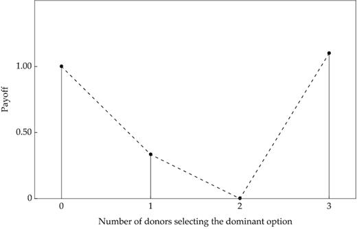
Payoffs as a Function of the Number of Donors Selecting Charity H.
Notes: δ = 1/10, F = 2, ϕ = 1/3.
Suppose next that each player can be one of two types, fully rational (R), or fully irrational (C), with the latter choosing one charity at random, i.e., each with a probability 1/2; and suppose that a donor’s type is private information. If the N donors are drawn at random from a large population where a fraction ζ of donors are of type C (and a fraction 1 − ζ are of type R), with ζ being the common belief among all donors, the probability (as seen from another player) of an individual donor being of type R—and thus selecting a charity on the basis of a payoff-maximising response to the choices of other players—is 1 − ζ, while the probability of an individual donor being of type C—and thus randomising between the two—is ζ.13
If donors can make mistakes in this way then option H is a comparatively ‘riskier’ co-ordination target than option L is, because if a single donor fails to co-ordinate on H, output is zero, whereas if a single donors fails to co-ordinate on L, output remains positive. On the other hand, if full co-ordination is successful, H dominates L. Note that at least three donors are required to generate this type of tradeoff: with only two players there are just three possible outcomes, and the only criterion for ranking H and L is payoff dominance.
Next consider a candidate equilibrium in which all players of type R co-ordinate on charity H, i.e., they all choose to give to H. If each of these donors conjectures that the probability of another donor choosing charity H is (1 − ζ) + ζ/2 = 1 − ζ/2 ≡ 1 − γ (γ = ζ/2), then from the point of view of each donor of type R who attempts co-ordination on H alongside the other R-type donors, the number of donors who will actually give to H will be three with probability (1 − γ)2, it will be two with probability γ(1 − γ) (with one donor giving to L), and it will be one with probability γ2 (with two donors giving to L). The associated expected payoff for a representative donor of type R considering co-ordination on H, if risk-neutral, is |$(1 - \gamma )^2\, (1 + \delta ) + (2\, \gamma ^2\, \phi )/(1 + 3\, \phi ) \equiv \hbox{EQ}_H$|. If, on the other hand, all players of type R attempt co-ordination on charity L, then, from the point of view of each of these donors, the number of donors who will actually give to L will be three with probability (1 − γ)2, it will be two with probability γ(1 − γ) (with one donor giving to H), and it will be two with probability γ2 (with two donors giving to H). The associated expected payoff for a risk-neutral representative donor of type R considering co-ordination on L, is |$(1 - \gamma ) \left(1 - \gamma \, (1 + \phi )/(1 + 3\, \phi )\right) \equiv \hbox{EQ}_L$|.
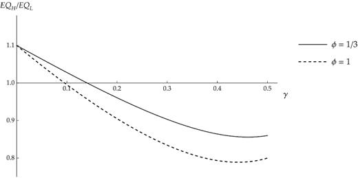
Ratio of Expected Payoffs under Full Co-ordination.
Notes: δ = 1/10, F = 2.
Figure 2 shows how the ratio EQH/EQL varies with γ for the same parameterisation that was used to generate Figure 1. In this case, for γ = 1/9 the full-coordination payoff for the dominant option is approximately equal to 0.87, whereas the corresponding payoff for the dominated option is approximately 0.86 < 0.87; for γ = 1/5 the ranking is reversed: 0.72 for the dominant option versus 0.75 > 0.72 for the dominated option. The effects of an increase in ϕ on the dominance ranking is illustrated in Figure 2, with reference to the example introduced earlier. Raising ϕ—which, by construction, leaves full-coordination payoffs unchanged—lowers the ratio EQH/EQL for any γ ∈ (0, 1/2], and can therefore overturn the ranking of expected payoffs. For example, for γ = 1/9, raising the fixed-cost premium to ϕ = 1 makes the full-coordination payoff for the dominant option approximately equal to 0.88, and that for the dominated option approximately equal to 0.89 > 0.88.
Risk aversion, if present, only works to strengthen the risk dominance implications of fixed costs. In the above example, for γ = 1/9, the ratio EQH/EQL is greater than unity under risk neutrality; if, however, output, Q, in each realisation is valued according to the Bernoulli utility function u(Q) = ln (1 + Q), we obtain E[u(Q)]H = 0.6 and E[u(Q)]L = 0.605 > 0.6, i.e., a comparatively lower γ is now required to overturn dominance.
The idea behind the notion of incumbency bias is that, in the presence of multiple equilibria, pre-existing co-ordination on any given choice makes that choice a natural choice (Samuelson and Zeckhauser, 1988). An incumbency bias/status quo bias effect such as this might thus provide protection to an incumbent charity against a challenger. The incumbent charity may be charity L (the high-cost, low-fixed cost charity), in which case incumbency would work to protect L against a more efficient, dominant challenger, i.e., incumbency would offset dominance; or it may be H (the low-cost, high-fixed cost charity), in which case incumbency would work to protect H against a less efficient, lower-fixed cost challenger, i.e., incumbency would offset the fixed cost-related risk advantage of charity L.
Incumbency bias can be formally incorporated into the preceding framework as a systematic departure by players of type C from a 50-50 choice rule, i.e., by assuming that players of type C select the incumbent charity with probability (1 + μ)/(2 + μ) > 1/2 (μ > 0) and the challenger with probability 1/(2 + μ). Thus if any given charity is the incumbent, and if players of type R co-ordinate on that charity, that charity will be selected by each of the other players with probability (1 − ζ) + ζ(1 + μ)/(2 + μ) = 1 − ζ/(2 + μ) ≡ 1 − γI; whereas if players of type R co-ordinate on the non-incumbent charity, it will be selected by each of the other players with probability (1 − ζ) + ζ/(2 + μ) = 1 − ζ(1 + μ)/(2 + μ) ≡ 1 − γN; and so γN = γ(1 + μ)/(1 + μ/2) > γ > γI = γ/(1 + μ/2). In other words, incumbency bias introduces an asymmetry between L and H in the perceived probability of mistakes, which in turn alters the comparison between full-coordination expected payoffs in favour of the incumbent.

Ratio of Expected Payoffs under Full Co-ordination – Incumbency Effects.
Notes: δ = 1/10, F = 2, ϕ = 1/3, charity L is the incumbent.
With reference to our earlier example, Figure 3 illustrates the effect of incumbency bias on the expected payoff ratio EQH/EQL for different values of γ, in a scenario where the payoff-dominated option, L, is the incumbent option. Incumbency of the low-fixed cost charity, L, lowers the minimum value of γ required to overturn dominance in its favour.
1.3. Quantal Response Equilibria
It can be shown that, other things equal, high fixed costs can negatively affect the equilibrium probability of selecting the dominant, high fixed-cost providers in a QRE.
In a left-hand neighbourhood of qH = 1, the level of qHin a stable equilibrium is a non-increasing function of the fixed cost premium, ϕ.
Thus, for qH high enough, an increase in the fixed cost gap between the two options, holding the full-coordination payoffs of the two options constant, (weakly) lowers the probability of individual players selecting the high fixed-cost, efficient option.15 Intuitively, a higher fixed-cost gap can make the dominated option comparatively less risky for any given qH, lowering the gap between a donor’s expected payoff from choosing H and L, and so, other things equal, the level of qH at which a donor is indifferent between selecting H and L must fall.
In Section 3 we use the QRE solution concept as a tool for interpreting our experimental results. Specifically, we derive structural estimates of the behavioural parameters of a QRE specification from experimental data, and then use those parameters to characterise the comparative statics properties of predicted equilibrium choices with respect to changes in cost parameters around the estimated equilibrium.
2. Implications for Competition and Entry
We now come to the heart of our discussion: how fixed costs in charity provision affect charity selection in charity markets. Our results so far imply that fixed costs can impede donor co-ordination on the more efficient provider—by skewing the dominance comparison against high fixed-cost providers and/or by lowering the mixed-strategy equilibrium probability of high fixed-cost providers being selected by donors. Implications for charities’ entry and exit choices immediately follow from our previous analysis.
Then, a charity’s calculation of whether or not it should participate involves a comparison between the payoff it obtains if it does not participate and the payoff it obtains if it does. The former payoff is zero if the other provider also chooses not to participate, and is otherwise equal to the payoff from full coordination on the alternative charity—which, by our normalisation equals unity for H if it is H that chooses not to participate and equals 1 + δ for L if it is L that chooses not to participate (with the alternative charity participating). The latter payoff is 1 + δ (for H) or 1 (for L) if the other provider chooses not to participate, and is otherwise equal to the payoff level that can be expected to arise in the binary choice problem as we have analysed it so far; in a QRE with mixing probability qH, this is equal to E[VH; qH] for provider H and E[VL; qH] for provider L.
If ω = 0, i.e., if charities are entirely pro-socially motivated, E[VH; qH] and E[VL; qH] coincide with each other and also with the common payoff that donors obtain. For qH strictly between 0 and 1, this common payoff is always less than the full-coordination payoff of 1 + δ that obtains when all donors select H or when H is the only provider. Not only is this payoff greater, but if one of the charities exits (or does not enter in the first place), this payoff obtains with certainty, and so this outcome unambiguously dominates all other outcomes. Thus, although the entry game may also admit equilibria where H exits (or does not enter),17 the favoured equilibrium for all parties is one where L exits (or refrains from entering), and so there need not be any competition failure.
If, however, ω > 0, then E[VH; qH] and E[VL; qH] are not the same. Since E[VH; qH] and E[VL; qH] are both increasing in ω, the payoff gaps that determine entry choices (E[VH; qH] − 1 for H and E[VL; qH] − (1 + δ) for L) are increasing in ω, implying that, if ω is large enough, outcomes will no longer be Pareto-rankable. Several different scenarios can then arise, some of which involve inefficient selection:18 (i) ω > δ but both E[VH; qH] < 1 and E[VL; qH] < 1 + δ, the entry game has a ‘Hawk-Dove’ structure, admitting two equilibria that cannot be Pareto ranked—with either H or L as the only provider; (ii) if E[VH; qH] > 1 and E[VL; qH] < 1 + δ, then the only outcome will be one where H is the only provider—the efficient outcome; (iii) if E[VH; qH] < 1 and E[VL; qH] > 1 + δ, then the only outcome will be one where L is the only provider—an inefficient outcome; (iv) if E[VH; qH] > 1 and E[VL; qH] > 1 + δ, then the only equilibrium outcome will be a duopoly—an inefficient outcome from the donors’ point of view.
In cases where L is the only provider—case (i), with H inactive, and case (iii), with L being the only provider—fixed costs translate into an inefficient entry barrier that protects the position of a less efficient provider. In case (iv), the duopoly outcome, fixed costs translate into a failure to repel inefficient challengers, making it possible for a less efficient provider to enter and survive competition. None of the above would be relevant to the entry choices made by for-profit providers: the only equilibrium outcome in the for-profit case would be one where H is the only active provider.
Note that by raising E[VH; qH] a higher ω could in principle improve selection if it brings about (ii) rather than (i). In other words, if a higher ω makes the efficient provider comparatively more combative and willing to participate, inducing exit by the less efficient provider, it could play a positive selection role. However, it can be shown that, other things equal, a higher ω raises entry incentives for the less efficient charity more than it does for the more efficient charity.
Provided that the dominance premium, δ, is sufficiently small, an increase in own provision bias, ω, raises the expected payoff of the less efficient provider – when it is chosen by donors with probability approaching unity—comparatively more than it increases the expected payoff of the more efficient provider—when it is chosen by donors with the same probability.
This implies that, ceteris paribus, an increase in ω is more likely to encourage entry by the low fixed-cost, inefficient provider (case (iii)) than by the high fixed-cost efficient provider (case (ii)), as the following example illustrates. Consider once more a scenario with N = 3, F = 2, δ = 1/10, ϕ = 1/3—the same as we considered in Subsection 1.2—and suppose that qH = 1/2. In this case, for ω < δ = 1/10 an outcome where H is the only provider is an undominated equilibrium; for ω between 1/3 and 2.85 there are two undominated equilibria, each with a single provider; for ω between 2.85 and approximately 4.45 the only equilibrium features L as the unique provider; for ω > 4.45, both providers participate; i.e., case (ii) never occurs. Intuitively, when donors select the two charities with equal probabilities, own provision bias bolsters the entry stance of the inefficient, low fixed-cost charity comparatively more, because it attaches a premium to positive levels of outputs which, for the same low level of donations, would be larger for the low fixed-cost charity.
Incumbency bias can affect entry outcomes simply because it affects the probability with which each donor selects a provider, raising it for the incumbent and lowering it for the challenger. It can therefore help offset selection failure (when the efficient provider is the incumbent), or it can exacerbate it.
If, additionally, own output-biased charities can select a technology from a set of available technologies, selection failure can take a different form: given that low fixed costs confer a competitive advantage, charities may choose to forgo the adoption of high fixed-cost technologies that allow them to exploit scale economies and opt for inferior technologies instead. When two competing providers have access to the same technologies, it immediately follows from the above analysis that, for ω sufficiently large, both providers would choose to enter and would select the inefficient, low fixed-cost technology, i.e., they would engage in a technological race to the bottom. Thus, not only can fixed costs impede efficient entry and exit, or allow inefficient entry and exit, but they could also impede efficient technology adoption and innovation.
3. Laboratory Experiments
We have designed and carried out two linked sets of experiments. The first set explores how fixed-cost based trade-offs lead to suboptimal choices of individual donors and co-ordination failures in giving and provides a direct test of the predictions contained in Section 1. The second set explores how donor co-ordination outcomes are reflected in entry and exit decisions, in line with the analysis of Section 2.
3.1. Donor Co-ordination Experiments
In Experiment 1 (the baseline experiment) of the set of donor co-ordination experiments, participants were asked to play 40 rounds of the following game: at the beginning of each round they are split into groups of three people each by a random draw;19 they are then asked to choose between two options, one of them (potentially) payoff dominant but involving a higher fixed cost, as discussed in the previous section.
Payoffs (derived from underlying cost parameters) were chosen so that deviation by a single player from the dominant option results in a payoff equal to zero. A representative payoff profile, as the number of players choosing the dominant option progressively increases from zero to three, has therefore the structure |$\big (x,\ \alpha \, x,\ 0,\ (1+\delta ) x\big )$|, with δ ≥ 0 and 0 ≤ α ≤ 1/2, with x, α and δ varying across treatments (the order is reversed in alternative treatments).20 Denoting with b each player’s notional contribution, the implied cost parameters, in relation to our earlier theoretical setup, are as follows: FH = 2b, cH = (b/x)/(1 + δ), FL = 3b − b/(1 − α) < FH, cL = (b/x)/(1 − α) > cH. The implied fixed-cost premium is therefore ϕ = α/(2 − 3α), which is positively related to α. The number of distinct experimental subjects who participated in the lab sessions is 102.
Laboratory experiments were conducted in the Behavioural Science Laboratory at Warwick Business School using the Decision Research at Warwick subject pool. For the first set of experiments, 102 participants were recruited. The majority of participants were undergraduate students at the University of Warwick: more than 70% of them studied Economics, Psychology or Business Administration; the rest were studying other subjects. The majority of participants had some experience with economic experiments, but none of them had taken part in similar experiments before. The average age was 21. Almost exactly half of the participants were male and half were female.21
The experiment was conducted using the experimental software z-Tree (Fischbacher, 2007). Upon arriving at the laboratory, each participant was seated at a workspace, equipped with a personal computer, scratch paper and a pen. The workspace of each participant was private; the session was monitored and any communication between participants was strictly forbidden. Participants received experimental instructions on a computer screen. At the beginning of a session, instructions were read aloud by the experimenter, and participants had an opportunity to re-read the instructions and ask individual questions. Participants were also asked to play a practice round; the payoff structure used in the practice round did not repeat any of the combinations used in the experiment. The experiment lasted approximately one hour. On average, participants were paid £11.30 inclusive of the show-up fee. In order to make sure that participants understood the games, in the post-experimental questionnaire we also asked them to indicate whether they found the experimental design challenging and/or to point out specific pathways for potentially improving the experimental design. None of the participants indicated having difficulties in understanding the design of the experiment. The majority of comments indicated that the instructions were ‘straightforward’ and ‘easy to follow’.
An additional set of 30 subjects used an online experimental portal for a treatment variant where payoffs were paid to an actual charity.
Twenty distinct payoff structures were used as a basis for the treatments in each round of the experiment. These are shown in Table 1, ordered in terms of number of players selecting the high-fixed cost option. Note that in some of those treatments we allowed for the low-fixed cost option to dominate the high-fixed cost option, i.e., we allowed for a negative δ. Accordingly, in the analysis of results we examine choices with reference to the level of fixed costs rather than dominance, but we draw a distinction between treatments where δ > 0 and those where δ < 0.
Payoff Treatments.
| No. of players selecting H | 0 | 1 | 2 | 3 |
|---|---|---|---|---|
| Payoff treatment | Payoffs | |||
| 1 | 200 | 100 | 0 | 200 |
| 2 | 200 | 100 | 0 | 201 |
| 3 | 200 | 100 | 0 | 205 |
| 4 | 200 | 100 | 0 | 210 |
| 5 | 200 | 100 | 0 | 215 |
| 6 | 180 | 50 | 0 | 175 |
| 7 | 180 | 50 | 0 | 180 |
| 8 | 180 | 50 | 0 | 181 |
| 9 | 180 | 50 | 0 | 185 |
| 10 | 180 | 50 | 0 | 190 |
| 11 | 150 | 70 | 0 | 145 |
| 12 | 150 | 70 | 0 | 150 |
| 13 | 150 | 70 | 0 | 155 |
| 14 | 150 | 70 | 0 | 160 |
| 15 | 150 | 70 | 0 | 165 |
| 16 | 175 | 25 | 0 | 145 |
| 17 | 175 | 25 | 0 | 160 |
| 18 | 175 | 25 | 0 | 175 |
| 19 | 175 | 25 | 0 | 190 |
| 20 | 175 | 25 | 0 | 205 |
Notes: H: high fixed-cost option.
For simplicity, and in order to ensure that players could easily understand the game and, at the same time, not be influenced by the framing of the experiment, the two available options were labeled as ‘Green Option’ and ‘Purple Option’. To control for possible order effects, the colour attached to the high fixed-cost option was randomised, and we also varied the displays shown to the participants: in some sessions payoffs were displayed in terms of increasing number of players choosing green over purple, and in other sessions the order was reversed. Thus, although we specified only 20 different payoff structures, the number of rounds each participant was asked to play was 40. The stranger design we adopted minimises learning effects. Furthermore, participants did not receive feedback about their payoffs from previous rounds until the very end of the experiment.
In most treatments, subjects were asked to choose one of the options without a default choice being made for them. In others (Experiment 2), a default choice is made for them, and subjects had the option of overturning it. We included this treatment variant in order to investigate incumbency effects. In Experiments 1 and 2, subjects were shown pre-calculated payoffs. In Experiment 3, subjects were required to derive the payoffs themselves on the basis of cost parameters and a set of detailed instructions.
Table 2 gives descriptive statistics for subjects’ choices (frequencies) in the base sample of 102 subjects across the 20 basic treatments, both in aggregate and broken down by incumbency treatment variant.
Experimental Choices: Choice Frequency for High-Fixed Cost Option (All Subjects).
| Payoff treatment | No default | L default | H default | All variants |
|---|---|---|---|---|
| 1 | 0.206 | 0.233 | 0.100 | 0.197 |
| 2 | 0.441 | 0.600 | – | 0.477 |
| 3 | 0.456 | 0.467 | 0.533 | 0.466 |
| 4 | 0.574 | 0.800 | 0.767 | 0.621 |
| 5 | 0.588 | 0.667 | 0.767 | 0.617 |
| 6 | 0.039 | 0.233 | 0.167 | 0.076 |
| 7 | 0.132 | – | 0.350 | 0.182 |
| 8 | 0.456 | 0.400 | 0.400 | 0.443 |
| 9 | 0.475 | 0.567 | – | 0.496 |
| 10 | 0.554 | – | 0.633 | 0.572 |
| 11 | 0.069 | – | 0.033 | 0.057 |
| 12 | 0.147 | 0.667 | 0.633 | 0.261 |
| 13 | 0.475 | 0.700 | 0.700 | 0.527 |
| 14 | 0.544 | 0.533 | 0.533 | 0.542 |
| 15 | 0.549 | 0.567 | 0.567 | 0.553 |
| 16 | 0.078 | 0.067 | 0.167 | 0.087 |
| 17 | 0.049 | 0.033 | – | 0.042 |
| 18 | 0.172 | 0.067 | 0.067 | 0.148 |
| 19 | 0.642 | 0.833 | 0.867 | 0.689 |
| 20 | 0.799 | 0.833 | 0.867 | 0.811 |
Notes: H: high fixed-cost option; L: low fixed-cost option.
Co-ordination performance is poor. If we calculate the corresponding mean payouts by treatment, we find that, on average, groups achieve a payoff that is only 58% higher than what would be achieved under fully random choices—if all players selected options at random each with probability of one-half. This is significantly less than what could be theoretically achieved if all players always co-ordinated on the dominant option—which would average to 177% more than the average payoff under random play. In other words, if we removed the dominated option from the set of options available to subjects, their average payoff would increase by more than 75%. If we removed the dominant option instead, the players’ average payoff would still increase by 66%.
To investigate the relationship between subjects’ choices and payoff structures, which reflect underlying technological differences, we can focus on normalised payoffs, which are derived as follows. Denoting with |$x^H_t$|, |$x^L_t$| and |$x^{PC}_t$|, in any given treatment t, respectively the full-coordination payoff for the high fixed-cost option (H), the full-coordination payoff for the low fixed-cost option, and the partial-coordination payoff associated with the low fixed-cost option (L), we compute Dominance Gap|$_t = x^H_t/x^L_t = 1+ \delta _t$|, and Fixed Cost Gap|$_t = x^{PC}_t/x^L_t = \alpha _t$| (which, as discussed before, is positively related to the fixed-cost premium).
If we focus on stable, mixed-strategy QR equilibria for the case N = 3, as shown in the proof of Proposition 2, the sign of the comparative statics effects of a parameter β (either the dominance premium, δ, or the fixed cost gap, α) on the mixed-strategy equilibrium probability of selecting H agrees with the sign of Ωβ(qH, β). For N = 3, we have |$\Omega _\delta (q^H,\beta ) = \lambda (q^H)^2\, \Xi$|, where Ξ ≡ exp (λ(EH − EL))/(1 + exp (λ(EH − EL)))2 > 0, which implies DqH/Dδ > 0; and |$\Omega _\alpha (q^H,\beta ) = \lambda \big (3 (q^H)^2-4 q^H +1\big )\, \Xi$|, which implies that DqH/Dα > 0 is negative if qH > 1/3 and positive or zero otherwise. In light of this, we could expect changes in δ across treatments to produce an effect of the same sign across treatments, and changes in α to produce effects of different sign depending on whether or not H is payoff dominant.
Table 3 presents results of random-effects logit panel regressions, where the dependent variable is the log of the odds of selecting the high fixed-cost option and the independent variables are the dominance gap (1 + δ), the fixed cost gap (α), and incumbency treatment indicators. For the reasons just discussed, we also include an indicator flagging those scenarios where option H is payoff dominated, and separate coefficients for α for treatments where H is dominant and treatments where H is dominated—as a rough way of allowing for the non-monotonicity implied by the theory. Column 1 of Table 3 shows results for the full sample, whereas column 2 focuses on the subsample of subjects who were asked to calculate payoffs.
Individual Choice: Panel Random-effects Logit Regressions Dependent variable: |$\hbox{logit}\big (\operatorname{Prob}\lbrace \hbox{Choice} = \hbox{High-fixed cost option}\rbrace \big )$|.
| Full sample | Subjects compute payoffs | |
|---|---|---|
| (1) | (2) | |
| Regressors | ||
| Dominance gap (H/L): 1 + δ | 15.599*** | 17.898*** |
| (1.356) | (2.388) | |
| H dominated | −3.267*** | −2.884*** |
| (0.371) | (0.600) | |
| Fixed cost gap if H dominant: α = 2ϕ/(1 + 3ϕ) | −1.165** | −2.207** |
| (0.475) | (0.775) | |
| Fixed cost gap if H dominated | 1.545* | 0.458 |
| (0.675) | (1.133) | |
| H default | 2.316*** | |
| (0.583) | ||
| L default | −0.152 | |
| (0.582) | ||
| Subjects must compute payoffs | 0.446 | |
| (0.557) | ||
| Constant | −16.103*** | −17.735*** |
| (1.542) | (2.623) | |
| Observations | 4,080 | 1,320 |
| Subjects | 102 | 33 |
| Fraction of variance due to individual effects | 0.614 | 0.526 |
Notes: Standard errors in parentheses.
*** p < 0.001, ** p < 0.01, * p < 0.05.
Looking at the full sample, the effect of the dominance gap on the probability of selecting H is positive and significant. The sign of the effect is as would be trivially expected, but the statistical significance of the effect indicates that individuals do trade off full-coordination payoff dominance against other considerations, rather than just choosing the payoff dominant option. The sign on the coefficient for α is negative and significant for treatments where H is dominant. This is in line with theoretical predictions. It is worthwhile stressing how this finding should be interpreted: our normalisation implies that changes in α do not affect the comparison between the two options in terms of their overall performance under full co-ordination—i.e., a higher fixed-cost gap, as measured by α, does not make H less efficient; nevertheless, it makes the choice of H less likely in those cases where H is the dominant option. In cases where H is dominated, the effect of a higher α is positive and significant. As noted above, this sign reversal is aligned with theoretical predictions.
Incumbency effects are as would be expected: incumbency of H has a positive and significant effect on the probability of H being selected, while incumbency of L has a negative effect; however only the first effect is statistically significant. Asking subjects to derive payoffs, or earmarking payouts to charity, has no significant effect in the full sample (column 1). Restricting the analysis to the subsample where subjects are asked to derive payoffs delivers strikingly similar results (column 2), suggesting that computational complexity (or lack thereof) does not play a central role in shaping behaviour. Augmenting the base sample with the additional 30 subjects whose payoff went to charity gives very similar results (not shown), with the ‘charity treatment’ indicator being not statistically significant.22
These results suggest that, even though subjects tend to avoid the high fixed-cost option, they are more likely to select it if it is presented to them as the default option. The fact that incumbency effects are not statistically significant for the low fixed-cost option is not surprising because subjects in our experiments tend to favour the low fixed-cost option over the high fixed-cost options anyway, and there is no reason we should expect subjects to favour the low fixed-cost option even more when it is presented as the default option.
We next carried out maximum likelihood estimation of the parameters of a QRE model as described in Subsection 1.3. We focused on three model variants: (i) one without incumbency effects, where the only structural parameter is λ; (ii) one with incumbency effects, with parameters λ and μ; (iii) one with both incumbency effects and with the payoff for the high-fixed restated as |${\tilde{x}}^H_t = x^H_t + \rho (x^H_t - x^L_t)$|, where ρ is a positive scalar that measures the marginal valuation of payout levels in excess of |$x^L_t$|, and which can depart from unity;23 this variant has three structural parameters: λ, μ and ρ. The reason for including specification (iii) is the observation, clearly evidenced by the descriptive statistics in Table 2, that subjects’ choices are dramatically affected by a switch in the dominance relationship between |$x^H_t$| and |$x^L_t$|: for example, when moving from payoff treatment 1 to 2, which both feature |$x^L_t = 200$|, a change in |$x^H_t$| from 200 to 201 raises the measured frequency of H being chosen from 0.206 to 0.441 in the no-incumbency treatment variant, but the effect of subsequent increases in |$x^H_t$|—as we move to payoff treatments 3, 4 and 5—is markedly less pronounced.
For every basic treatment, we have at most two observations per subject, and so no individual-specific parameter estimation is possible. Accordingly, in performing the estimation, the choices of individual subjects for any given treatment were pooled in a single sample.24
Maximum likelihood parameter estimates are shown in Table 4, which also shows likelihood ratios for moving from one specification to the next, progressively adding one parameter to the previous one. The implied value of λ is consistently around 0.012. Adding incumbency effects significantly improves the model’s fit to the experimental data. Allowing for non-linearities above |$x^L_t$| further improves the fit; more importantly, it brings predicted equilibrium values of qH closer to the 1/3 critical point—above which the effect of a higher fixed-cost premium on qH is non-positive, consistently with the results of the previous panel estimation results—for a larger subset of treatments where option H is the payoff dominant option.
Maximum Likelihood QRE Estimates.
| Specification | |||
|---|---|---|---|
| Parameter | (i) | (ii) | (iii) |
| λ | 0.0123 | 0.0125 | 0.0115 |
| μ | – | 0.1725 | 0.1425 |
| ρ | – | – | 2.98 |
| Incremental likelihood ratio | – | 212.2 | 115.8 |
| Observations | 4,080 | 4,080 | 4,080 |
| Specification | |||
|---|---|---|---|
| Parameter | (i) | (ii) | (iii) |
| λ | 0.0123 | 0.0125 | 0.0115 |
| μ | – | 0.1725 | 0.1425 |
| ρ | – | – | 2.98 |
| Incremental likelihood ratio | – | 212.2 | 115.8 |
| Observations | 4,080 | 4,080 | 4,080 |
Notes:(i) No incumbency effects.
(ii) Incumbency effects.
(iii) Incumbency effects + change in valuation above |$\, \min \lbrace x^L, x^H\rbrace$|.
Table 5 shows predicted choice frequencies corresponding to specification (iii) under the estimated parameters, alongside actual frequencies. Out of the 20 basic payoff treatments we investigate, and with reference to observations for cases in which there is no incumbency treatment, observed frequencies for all 20 scenarios are ‘right’ in relation to the predicted comparative statics effects, i.e., they exceed 1/3 in treatments where the high fixed-cost option is also the payoff dominant option or fall short of 1/3 in treatments where the high fixed-cost option is the payoff dominated option—implying that in all scenarios a higher normalised fixed-cost premium (holding δ constant) is predicted to lower the probability of choosing H, as is indeed implied by our earlier regression results. Of the predicted frequencies from the QRE estimation, 13 out of 20 are on the right side of 1/3, and only two out of 20 are on the wrong side of 1/3 by more than 10%—i.e., less than 0.3 if H is dominant and greater than 0.367 if H is dominated. In other words, there are no clear outliers that are obviously at odds with an augmented QRE specification. In 75% of all cases the sign of the experimental effect on choice frequency of moving from one game to another—a total of 20 × 19 possible comparisons, shown in Appendix A, Table A 3—agrees with the effect that is predicted by the theory.
Predicted and Actual Choice Frequencies—Choice of Option H (Laboratory Subjects Only).
| No default | L default | H default | All variants | |||||
|---|---|---|---|---|---|---|---|---|
| Payoff treatment | Predicted | Actual | Predicted | Actual | Predicted | Actual | Predicted | Actual |
| 1 | 0.303 | 0.201 | 0.259 | 0.167 | 0.363 | – | 0.290 | 0.191 |
| 2 | 0.304 | 0.431 | 0.259 | 0.433 | 0.366 | 0.767 | 0.291 | 0.480 |
| 3 | 0.309 | 0.472 | 0.262 | 0.500 | 0.377 | – | 0.295 | 0.480 |
| 4 | 0.316 | 0.556 | 0.266 | – | 0.841 | 0.783 | 0.471 | 0.623 |
| 5 | 0.816 | 0.576 | 0.270 | – | 0.899 | 0.717 | 0.841 | 0.618 |
| 6 | 0.324 | 0.035 | 0.260 | – | 0.428 | 0.200 | 0.355 | 0.083 |
| 7 | 0.335 | 0.118 | 0.265 | 0.100 | 0.478 | 0.600 | 0.377 | 0.186 |
| 8 | 0.338 | 0.410 | 0.266 | 0.400 | 0.495 | – | 0.317 | 0.407 |
| 9 | 0.350 | 0.444 | 0.271 | 0.500 | 0.724 | 0.633 | 0.327 | 0.480 |
| 10 | 0.371 | 0.528 | 0.277 | 0.567 | 0.832 | 0.700 | 0.507 | 0.559 |
| 11 | 0.372 | 0.069 | 0.321 | 0.017 | 0.435 | – | 0.357 | 0.054 |
| 12 | 0.383 | 0.146 | 0.328 | – | 0.454 | 0.650 | 0.404 | 0.294 |
| 13 | 0.395 | 0.444 | 0.335 | – | 0.480 | 0.700 | 0.420 | 0.520 |
| 14 | 0.411 | 0.542 | 0.343 | 0.533 | 0.518 | – | 0.391 | 0.539 |
| 15 | 0.432 | 0.535 | 0.352 | 0.567 | 0.601 | – | 0.408 | 0.544 |
| 16 | 0.285 | 0.049 | 0.231 | – | 0.358 | 0.117 | 0.307 | 0.069 |
| 17 | 0.310 | 0.042 | 0.242 | 0.017 | 0.420 | – | 0.290 | 0.034 |
| 18 | 0.357 | 0.146 | 0.257 | 0.067 | 0.694 | – | 0.327 | 0.123 |
| 19 | 0.841 | 0.681 | 0.279 | – | 0.883 | 0.850 | 0.854 | 0.730 |
| 20 | 0.930 | 0.826 | 0.912 | – | 0.943 | 0.850 | 0.933 | 0.833 |
Notes: H: high fixed-cost option; L: low fixed-cost option
Predicted performance based on QRE specification (iii), with incumbency effects and non-linear valuation.
3.2. Experiments on Entry/Exit Choices
To explore implications of co-ordination outcomes on entry/exit choices, we designed a second set of experiments that built on the co-ordination experiments presented in Subsection 3.1. We asked subjects to choose between a safe prospect that corresponded to the full co-ordination outcome for one of the two options in the previous co-ordination experiment, and a risky prospect that involved all four possible co-ordination outcomes from the co-ordination game, each occurring with a probability that was equal to its experimental frequency (from the previous experiment). The safe prospect was the outcome that would prevail if only one of the two giving options was present, i.e., if one of the two charities chose not to participate—either by exiting or by not entering in the first place. The risky prospect was what individuals faced ex ante if both options were present, i.e., if both charities participated.
We divided participants into groups of four people each. Each group consisted of players of two types: one player was appointed to choose between the safe and the risky prospect (decision-maker), while three players acted as passive recipients of that choice (passive recipients). These types were assigned randomly at the beginning of each experiment and stayed the same through all treatments. Including passive recipients enabled us to account for the possible effects of other-regarding preferences on the choice of the decision-maker.
We also incorporated departures from pure pro-social motivation by allowing for the decision-maker to attach a premium ω ≥ 0 to one of the two donation options from which the safe and risky prospects are derived—producing different payoffs for the decision-maker in comparison with those of the passive recipients.
We focused on a subset of eight games among those we used for our previous experiments—games 3, 5, 13, 15, 23, 25, 33, and 35—and for each of these we examined four types of treatments. In each of these treatments, the risky prospect for the receivers was obtained by combining the point payoffs corresponding to each outcome for the game with the empirical probabilities obtained from the experiments presented in Subsection 3.1.25 The risky prospect for the decision-maker in treatments 1 and 2 was calculated by taking the same empirical probabilities and multiplying the point payoff in outcome 1 for receivers by 1 + ω and keeping the rest of point outcomes the same as those of receivers. The risky prospect for the decision-maker in treatments 3 and 4 was calculated by taking the same empirical probabilities and multiplying the point payoffs in outcomes 3 and 4 for receivers by 1 + ω. The point payoff for the decision-maker in the safe option was also multiplied by 1 + ω if it corresponded to a full co-ordination outcome to which the decision-maker attached a premium in the given treatment. The experiment incorporated 320 questions (160 in the individual task and 160 in the group task). It lasted 1.5 hours and each participant received, on average, £25.
The structure of these treatments is illustrated in Table 6, which refers to game 15 in the previous experiments and assumes a premium ω = 0.2 on the H option for the decision-maker. As detailed earlier, in game 15 each member of the three-person group receives 190 points when all group members co-ordinate on the H option (outcome 1); nothing if two out of three group members co-ordinate on option H and one group member opts for L (outcome 2); 50 points if one out of three group members opts for H and two co-ordinate on L (outcome 3); and 180 points if all three group members co-ordinate on option L (outcome 4). We base the probability (frequency) of observing each of the possible four outcomes on the results of our previous experiments: for game 15; these probabilities are 0.18, 0.47, 0.29 and 0.06, corresponding to outcomes 1, 2, 3 and 4, respectively. The payoffs that the passive recipients (denoted as PRs in Table 6) obtain in each realisation under the risky prospect are simply 190, 0, 50, 180, whereas the decision-maker attaches a premium ω = 0.2 to payoffs obtained from the H option in treatments 1 and 2 and to payoffs obtained from the L in treatments 3 and 4, giving rise to a different payoff profile for the decision-maker (denoted as DM in Table 6). The safe prospect reflects either the full co-ordination outcome for H or for L, yielding different payoffs for the decision-maker and the passive recipients in treatments where the decision-maker attaches a premium to the corresponding option.
Entry/Exit Experiments: Treatment Payoffs for Game 15 and for ω = 0.2.
| Risky Prospect | Safe Prospect | |||||
|---|---|---|---|---|---|---|
| Outcome 1 | Outcome 2 | Outcome 3 | Outcome 4 | |||
| Treatment | Player(s) | |$\Pr =0.18$| | |$\Pr =0.47$| | |$\Pr =0.29$| | |$\Pr =0.06$| | |$\Pr =1$| |
| 1 | PRs | 190 | 0 | 50 | 180 | 190 |
| DM | 228 | 0 | 50 | 180 | 228 | |
| 2 | PRs | 190 | 0 | 50 | 180 | 180 |
| DM | 228 | 0 | 50 | 180 | 180 | |
| 3 | PRs | 190 | 0 | 50 | 180 | 190 |
| DM | 190 | 0 | 60 | 216 | 190 | |
| 4 | PRs | 190 | 0 | 50 | 180 | 180 |
| DM | 190 | 0 | 60 | 216 | 216 | |
Notes: PRs: passive recipients; DM: decision-maker
In Treatment 2, the subject appointed to make the choice places a premium on the high fixed-cost, efficient option in the risky prospect. This treatment can be thought of as corresponding to scenarios where the high fixed-cost, efficient charity must make a choice between remaining active and competing with a less efficient, lower fixed-cost challenger or conceding to it (which amounts to inefficient exit). In Treatment 3, the subject appointed to make a choice places a premium on the low fixed-cost, inefficient option in the risky prospect. This treatment can be thought of as corresponding to scenarios where the low fixed-cost, inefficient charity must make a choice between conceding to a more efficient, higher fixed cost challenger or remaining active and competing with it (which amounts to inefficient entry). In treatments 1 and 4, the riskless option coincides with the option to which the chooser attaches a premium, making it comparatively more attractive to the decision-maker than to the passive recipients. Unlike treatments 2 and 3, these two treatments do not naturally map into entry/exit choice scenarios, but are nevertheless included for the sake of symmetry and for diagnostic purposes.
We include these four treatments for each of the eight games and for five different values of ω (ω = 0, 0.01, 0.05, 0.1 and 0.2), ending up with a total of 160 treatments. Each player who was chosen to be a decision-maker took part in all 160 treatments. For each of these 160 treatments, we include two treatment variants: one in which there are no implications for other subjects, the other where the choice has payoff implications for other (fully passive) subjects, with the chooser being aware of those implications—this allows us to account for the possible role of other-regarding motives for entry/exit choices.
A total of 60 participants were recruited for the second set of experiments—all undergraduate students at the University of Warwick, as for the first set of experiments. The 60 subjects were randomly allocated to 15 groups of four people each. This means that, of all 60 subjects, 15 acted as decision-makers and the rest as passive recipients.
Inefficient entry by the low fixed-cost, high average cost charity occurs in 23% of the cases for treatments that correspond to this scenario (i.e., treatments in which the chooser attaches a strictly positive premium to the low fixed-cost choice in the risky prospect). When choosers are also asked to take into account payoff consequences for other subjects, this proportion falls to 3.5%, and the difference is statistically significant—at the 1% level according to a Wilcoxon signed-rank test. Inefficient exit by the high fixed-cost, low-average cost charity occurs in 46% of the cases for treatments that correspond to this scenario (i.e., treatments in which the chooser attaches a strictly positive premium to the high fixed-cost choice in the risky prospect). When choosers are also asked to take into account payoff consequences for other subjects, this proportion falls to 37.5%, and the difference is again statistically significant at the 1% level. Thus, making the payoff consequences to other subjects salient to the decision-maker seems to induce the decision-maker to give comparatively more weight to the payoff dominant option—in the first case by choosing it as a safe option, and in the second case by forgoing the payoff-dominated safe option.
4. Discussion
Our analysis has intentionally abstracted from a number of real-world complications as well as from possible alternative interpretations.26 We touch on some of these below.
4.1. Experimental Complexity and Framing Effects
When interpreting our experimental results, a possible concern is that the mis-coordination we observe may just follow from the relative complexity of the experimental setting rather than from the trade-offs highlighted in our theoretical discussion, and might not arise in a simpler (and possibly more realistic) choice situation. As a robustness check, we have conducted an additional two sets of laboratory experiments, with subjects selected from a population comparable to that of our main experiments.27
The first set of experiments incorporated a ‘stag hunt’ game with the payoff structure shown in panel (i) of Table 7—a well-known game in which players may react to risk dominance by co-ordinating on a payoff-dominated choice, as in our main co-ordination experiment. When confronted with this situation, 59.3% of 32 subjects who took part in this treatment (19 of 32), selected the payoff-dominated option (A).
Payoff Structures for Reduced Complexity and Framing Treatments.
| (i) | (ii) | ||||
|---|---|---|---|---|---|
| A | B | A | B | ||
| A | 8,8 | 4,0 | A | 8,8 | 4,4 |
| B | 0,4 | 9,9 | B | 4,4 | 9,9 |
| (i) | (ii) | ||||
|---|---|---|---|---|---|
| A | B | A | B | ||
| A | 8,8 | 4,0 | A | 8,8 | 4,4 |
| B | 0,4 | 9,9 | B | 4,4 | 9,9 |
This particular example, however, cannot be directly linked to the public good problem that we have studied, because in a public good game with only two players the presence of fixed costs cannot generate a payoff structure exhibiting risk dominance—at least three players are needed. A two-player version of the game we study can only exhibit payoff dominance, as in panel (ii) of Table 7. Still, we can use this to gauge whether, in a simple two-player choice situation, subjects fail to co-ordinate on a Pareto-dominant option even when there is no trade-off with risk dominance. Experimental results indicate that mis-coordination can occur even in this case: 29.4% of subjects choose the payoff-dominated option (A).28 Yet, statistical tests clearly show that mis-coordination in the ‘stag hunt’ game is much more prevalent than in this case.29
To understand the role of framing effects in relation to fixed costs—the possibility that the very idea of fixed costs may trigger aversion independently of the effects that fixed costs have on payoffs—we examined four treatment variants of (i) and (ii) in which subjects were told that the differences between A and B were generated by fixed costs. As discussed, a public goods game with fixed costs is not capable of generating the payoffs in (i); nevertheless attaching a fixed-costs ‘label’ to alternatives may still produce framing effects that are independent of the effect of fixed costs on payoffs. When we told subjects that B (the payoff dominant option) involved costs, fewer subjects chose B in both (i) and (ii): framing increased the proportion of subjects choosing A from 59.3% to 70.6% in game (i) and from 29.4% to 43.3% in game (ii). When we instead told subjects that A (the payoff-dominated option) featured fixed costs, fewer subjects chose A: the proportion of subjects choosing A decreased from 59.3% to 50% in game (i) and from 29.4% to 20% in game (ii). But statistical tests reveal that in all cases the changes induced by framing are not statistically significant. In contrast, as we have just seen, the structure of payoffs matters and effects are statistically significant when we compare play in (i) and (ii); and so, if fixed costs give rise to a payoff structure that involves a payoff-versus-risk dominance trade-off, as they do in our main experiments with N > 2, we should expect them to have an effect on choices that goes beyond mere framing effects.
4.2. Large Donor Pool
Fixed costs of any given size become negligible if variable costs become increasingly large due to an expansion of output, e.g., because the number of donors is large. Although this is formally true in our simple model specification, in practice inframarginal costs do scale up with the level of operation. For example, we would not expect a large manufacturer to incur the same inframarginal costs as a small workshop; and the same would apply to charities. Indeed, looking at charities’ balance sheets, we see that (unsurprisingly) categories of costs—such as managers' salaries or rental payments—that are correlated with fixed costs do increase with the size of a charity. Thus, operation on a large scale with the support of a large number of donors does not imply that inframarginal costs must be a negligible fraction of total donations.
This positive relationship between size and inframarginal costs can arise from a menu of technologies with varying fixed and marginal costs, with providers selecting higher fixed-cost, lower marginal-cost technologies as they expand their scale of operation, implying that the ratio of fixed to total costs does not become negligibly small as donation size becomes large.30 Alternatively, it may reflect the need for lumpy, short-run capacity investment costs: fixed costs could then scale up with the size donor pool but would be given when examining the choices of the marginal N donors—the choices we are focusing on in our analysis.31
As we discussed in Subsection 1.3, independently of technological considerations (i.e., if opportunities for exploiting scale economies do not scale up with the volume of provision), co-ordination can still be partial even if the number of donors is large.
4.3. Output Differentiation
Donors may view the activities of competing charities as being imperfect substitutes, i.e., as differentiated goods. Then, as is the case for private-sector competitors that produce differentiated varieties, incurring the fixed costs required to produce additional varieties may be warranted and socially optimal. For private goods the trade-off between the benefit of additional varieties and the additional costs involved can be resolved efficiently by market competition—as characterised by the mainstream models of monopolistic competition under product differentiation (e.g., Dixit and Stiglitz, 1977). As already noted, however, the mechanics of price competition do not readily carry over to the not-for-profit case.32
While a single-provider outcome may not be necessarily the efficient outcome in this case, donors would still face a co-ordination problem, and charities that are own-output biased may still leverage on this co-ordination problem to displace more efficient charities, which would result in above-optimal differentiation and suboptimal exploitation of economies of scale.
4.4. Unobservable Technologies
The preceding discussion has assumed that donors can directly observe charities’ technologies, which is unlikely to be the case. It may be comparatively easier for donors to observe fixed costs (as they may materialise in the form of expenditures that are comparatively more visible), whereas marginal costs may be harder to observe directly, and could only be inferred from provision outcomes if full co-ordination were actually to occur. What our analysis has shown is that, even if average-cost dominance is fully salient to donors, co-ordination of donations towards lower-average cost charities that have higher fixed costs can be difficult to achieve; but if marginal costs are unknown to donors, one might expect charity selection to be driven even more by fixed costs if these are observable.
4.5. Communication, Core Grants, Large Donors
In co-ordination games, communication among players can in principle support the selection of a Pareto-dominant outcome. In the institutional context we are studying, communication would occur through the fundraising of charities and volunteers; if these are biased, multiple and competing signals will be sent, and there is no presumption that communication should make efficient selection more likely (Cooper et al., 1992).
The co-ordination problem we have studied arises from the need to cover comparatively large fixed costs with comparatively smaller individual donations; and so it could be mitigated or eliminated if core costs were funded by larger lead donations from large donors (Gneezy et al., 2014). Absent large donors, there may be a role for government to step in and do the same through ‘core’ grants. But if these grants are given indiscriminately to all charities and consist of funds that are redirected from the overall pool of available funding, reducing the size of the remaining donations (as would be the case under a hypothetical intervention that taxes all donations and splits revenues equally across the two charities); and if they are still not large enough to fully cover fixed costs, their effect would actually be to raise the relative gaps in residual fixed costs, which could exacerbate the donor co-ordination problem.33
4.6. Endogenous Contribution Levels
In our analysis we have deliberately abstracted from the choice of contribution levels, focusing on the co-ordination problem that fixed costs entail in isolation from other dimensions of donors’ choices. Nevertheless, the co-ordination problem can be expected to affect the volume of donations.
Contribution performance is so poor in our laboratory experiments that it could be improved simply by restricting the choice to either charity. Then, if donors have the option to withhold their contribution and direct it towards private consumption instead, they will be more likely to do so when multiple options are available—i.e., co-ordination failure across donors may also translate into a reluctance to give.
To see this, consider a setting in which contributors have the option of not giving at all—a discrete choice between giving and not giving—but where the private opportunity cost of giving, ν, for the marginal donor is less than the marginal private benefit, i.e., ν < 1/cj, j ∈ {1, 2}. This means that provision does not entail free riding, and so an outcome where all donors make positive contributions to either charity is a Nash equilibrium; however, if fixed costs are large enough, an outcome with no contributions is also an equilibrium. Suppose then that, in this setting, donors face a single option that involves fixed costs, and compare this scenario with one in which donors face two fixed-cost options—as in the second set of experiments described in the previous section but with contribution levels now being endogenous. In both scenarios, depending on parameter values, a no-contributions outcome could be a Nash equilibrium. However, if donors anticipate that having multiple options lowers the expected return of marginal contributions (in line with our predictions on provision performance), they would be less willing to contribute, making a no-contribution outcome (or a low-contribution outcome) more likely when multiple providers are present.
4.7. Other Negative Connotations of Fixed Costs
Donors may dislike fixed costs for reasons that have nothing to do with the arguments that we have presented. For example, in the presence of moral hazard, fixed costs may be taken by donors as a signal that funds are misused by charity managers—if managers obtain more ‘ego rents’ or personal perks from fixed expenditures than from programme expenditures (although it must be said that opportunities for misuse and misappropriation of funds are just as great for variable expenditures). Or it may be that the extent of the ‘warm glow’ (Andreoni, 1990) that donors experience from their donations varies depending on the perceived destination of the donation.
While it is possible that other considerations play an important role in shaping how donors respond to charities' fixed costs, even when these considerations are absent—as they are, by design, in both our theoretical and experimental settings—fixed costs can drive donors away and can lead to inefficient selection. If donors have additional reasons for disliking fixed costs, those will only add to the effects that we have described.
5. Concluding Remarks
Our analysis has shown that, absent a residual claimant, selection of the most efficient charity cannot be guaranteed: unlike in the case of for-profit firms, the presence of fixed costs may interfere with competition among non-commercial, not-for-profit providers and give rise to inefficient selection. Experimental evidence suggests that donors’ co-ordination and contribution performance can be adversely affected by the presence of fixed costs, that this effect can be significant, and that donors can be biased against higher-fixed cost providers even if these are more efficient—which undermines contestability in charity markets.
The debate on the effects of government funding on the private provision of public goods and services has so far largely ignored the effects of government funding on intercharity competition and market structure in the third sector. Our conclusions imply that, once entry and technology adoption decisions are accounted for, there is no longer a theoretical prior that government grants that are directed towards charities’ core funding needs should be neutral, i.e., that they should simply crowd out private donations. On the contrary, government grants might be able to affect entry and/or charities’ technology choices—and hence provision efficiency.
Specifically, selective government subsidisation of fixed costs may then be required to promote efficient selection of service providers (with the caveat we mentioned in Section 2). ‘Funding of charities’ fixed costs can be expected to dominate direct regulation as away of promoting efficient selection, as the latter would require the government to have full information on the technologies of individual providers; but it still requires an assessment of the comparative severity of the two kinds of failures related to competition and entry. If established charities are technologically entrenched and rely on unnecessarily high fixed-cost technologies, and entry by start-ups can lead to the adoption of more efficient technologies, then government funding of core costs should be directed towards start-ups; if instead start-ups are higher-cost, opportunistic challengers that can take advantage of the higher fixed costs of more efficient, more established charities in order to divert private funds their way, making it difficult in turn for established charities to fully exploit opportunities for economies of scale in provision, then funding the core costs of established charities should take priority.’
Government funding choices do appear to be sensitive to charities’ core funding needs,34 but it is not clear whether this is motivated by the need to promote entry by new charities—overcoming the implicit entry barriers that fixed costs can create—or instead by the need to support efficient technology adoption by incumbents.35
Additional Supporting Information may be found in the online version of this article:
Online Appendix
Replication Package
Notes
We wish to thank Gani Aldashev, Jim Andreoni, Richard Blundell, Maitreesh Ghatak, Alex Imas, Judd Kessler, Andreas Lange, Clare Leaver, Jonathan Meer, Paul Niehaus, Mark Ottoni-Wilhelm, Ragan Petrie, Imran Rasul, Thierry Verdier, Huseyin Yildirim and participants at the conferences and seminars at Bristol, Duke, Hamburg, Helsinki, London, Manchester, Munich, Ottawa, Victoria, Warwick for comments and suggestions. Research support from CAGE (Warwick) and the Economic and Social Research Council is gratefully acknowledged. Ganna Pogrebna acknowledges financial support from RCUK/EPSRC grants EP/N028422/1 and EP/P011896/1.
Footnotes
Spends on direct programme costs reported by UK charities range from 1% to 65% of their income (True and Fair Foundation, 2015).
As Rosemary McCarney, CEO of Plan Canada, put it, ‘There’s an idea out there that a charity is good if it only spends 20% on administration and fundraising and 80% on program costs, and if you’re out of that approximate range, somehow you’re bad or inefficient.’ Often the ratio of variable to fixed costs is taken as an indicator of provision efficiency (see, for example, the charity rating system adopted by MoneySense, a not-for-profit Canadian consumer advocacy organisation).
The difficulties that charities face in persuading donors (especially small ones) to make donations that are not earmarked towards project costs and can be used to fund core costs leads charities to formulate specific core funding strategies. See, for example, Institute for Philanthropy (2009). Gneezy et al. (2014) also note that donors are averse to making donations to charities that have large overhead costs, and show that large donations earmarked towards overhead costs can be effective at overcoming this aversion. However, they do not address the implications of differential cost structures for donor co-ordination, as we do here.
A commercial firm’s bottom line only matters to its customers if sales contracts involve long-term components, e.g., an advance payment for later delivery or important maintenance and warranty elements. In the vast majority of cases, the bulk of the delivery of goods and services takes place at the time of sale.
These dimensions include information and agency costs (Alchian and Demsetz, 1972; Hansmann, 1980; Easley and O’Hara, 1983; Glaeser and Schleifer, 2001); differential regulatory and tax regimes (Lakdawalla and Philipson, 2006); and access to a pro-socially motivated workforce (Ghatak and Mueller, 2010).
A number of studies have focused on the implications of fundraising efforts (Rose-Ackerman, 1982; Castaneda et al., 2008; Aldashev et al., 2014). Other studies have focused on the regulation of intercharity competition in non-contestable markets (Philipson and Posner, 2009) and on the implications of adverse selection for charity selection (Scharf, 2014; Kasteva and Yildirim, 2016).
In a dynamic setting, short-run profits can be positive or negative even when there is a non-distribution constraint, but profits must be zero in the long run. However, in our static framework, a non-distribution constraint translates directly into a zero-profit constraint. In the language of Hansmann (1980), such providers are donative non-profits.
With collective consumption, overall output may be difficult to verify even when deliveries to individual purchasers are fully verifiable. This makes the verification problem comparatively more likely to occur in the case of collective goods, as the following example illustrates. Suppose that two individuals each contribute an overall amount v towards provision of a purely collective service with marginal cost c = 1; even if each contributor is able to verify that an amount v is provided as a direct consequence of her own individual contribution, she may be unable to verify that an additional amount v is also provided as a result of the other individual’s contribution. In this case, the provider may be able to supply a total amount v (rather than an amount 2v) and still satisfy its contractual obligations with each of the two contributors.
We therefore assume that provision cannot become negative—or equivalently, that if the difference between donations received and Fj is negative, this difference can be funded in some way (privately or by the government). An alternative assumption that leads to the same conclusion is that whenever a charity receives donations that fall short of Fj, it does not directly engage in provision and instead diverts the donations it receives towards another charity.
Analogous inefficiencies can arise for not-for-profit firms that price at average cost, e.g., consumer co-operatives (Enke, 1945).
Andreoni (1998) points to fundraising as a possible solution to the problem of achieving co-ordination among donors in the presence of a donation threshold. In the setting that we study here, the total level of donation is given, and so fundraising cannot alter the structure of the problem: two non-passive charities that place a premium on their own provision would both face similar incentives to exert effort in targeting donors.
The resulting game is one of incomplete information and the relevant equilibrium concept is Bayes-Nash equilibrium. However, we use this construct here to build intuition with respect to the dominance ranking, not as a way of characterising equilibria. To the latter end, in Subsection 1.3 we invoke the concept of Quantile Response Equilibrium (QRE; McKelvey and Palfrey, 1995), which is a technically more suitable (if perhaps less intuitive) solution concept in this context. The above construct can also be viewed as a special case of a level-k reasoning framework (Stahl and Wilson, 1994), where level-0 players randomise between the two charities and level-1 players best-respond to an assumed distribution of level-0 and level-1 players in proportions ζ and 1 − ζ.
Accordingly, for λ approaching infinity, the game admits two stable pure-strategy equilibria and an unstable mixed-strategy equilibrium. For λ finite, different equilibrium set typologies can arise: (i) multiple equilibria of which only the pure strategy ones are stable (for λ large); (ii) multiple mixed-strategy equilibria of which some are stable (as λ becomes smaller); (iii) a single, stable mixed-strategy equilibrium (as λ becomes even smaller).
The conditions for qH to be strictly increasing in ϕ need to be separately derived for each N; in Section 3 we will focus on the case N = 3 and discuss conditions for that case.
It should be noted that a larger number of donors does not necessarily translate into the requirement of a smaller λ (i.e., donors being more ‘irrational’) for mis-coordination to occur. For example, with F = 2, δ = 1/2, ϕ = 1/3, λ0 = 1,000 and N0 = 3, there is a stable QR equilibrium featuring qH ≈ 0.937. If we raise the number of donors to N = 4, the value of λ required for qH ≈ 0.937 to remain an equilibrium is λ ≈ 5, 791 > 1,000. As we discuss later in Section 4, we should also expect a larger donor pool to be associated with larger inframarginal costs.
If qH is such that E[Q; qH] < 1, then an outcome where L enters and H does not enter is also an equilibrium.
N = 3 is the smallest level of N for which there can be asymmetric, partial co-ordination outcomes (i.e., more donors co-ordinating on one charity than on the other, short of full co-ordination).
A zero payoff may be perceived by subjects as being especially salient; this would have an effect analogous to that of risk aversion (e.g., it would be tantamount to the zero payoff being ‘counted’ by subjects as a negative payoff, rather than a zero); but it would not change our theoretical predictions nor our interpretation of the experimental results. In the maximum likelihood estimation exercise we discuss below, we allow for non-linearities.
Detailed statistics about the first set of experiments are provided in Appendix A, Table A1.
An alternative way of looking at experimental evidence is to focus on the probability of selecting the dominant option, which coincides with H in some treatments and with L in others. Under this specification, the combination of a negative effect of α on the probability of choosing H when H is dominant and a corresponding positive effect when H is dominated, would translate (by construction) into a negative effect of a higher α on the probability of choosing the dominant option in all cases. Results from this specification (not shown) are indeed in agreement with those of Table 3.
This non-linear specification can be interpreted as implying loss-aversion/loss-loving, with |$x^L_t$| identifying subjects’ reference point.
Also note that, since multiple (stable) strictly mixed-strategy equilibria are possible for any given treatment and parameter configuration, the estimation procedure involves selecting the combination of equilibrium values across all treatments that delivers the maximal likelihood value for the given parameter configuration; and then, given those maximal values, selecting the parameter configuration that delivers the maximal overall likelihood value.
Details of the games and of the choice probabilities derived from the first set of experiments are given in Appendix A, Table A4.
Empirically identifying (outside the lab) the effects that we investigate here would need to account for these complications. This is challenging, mainly because data on charities’ technology choices is scarce. The Canadian dataset previously mentioned is unique in providing a systematic account of the structure of charities’ balance sheets; but, as noted earlier, information on balance sheets does not easily translate into information on provision technologies.
An additional 190 undergraduate students at the University of Warwick were recruited through the Decision Research at Warwick (DR@W) subject pool. Of these, 47% were female. None of the participants had taken part in a similar experiment before. The experiment lasted 15 minutes and participants received £7 on average (inclusive of the show-up fee).
Thirty-four of our subjects played this treatment.
Both a Pearson χ2 test and a one-sided Fisher’s exact test show significance at the 5% level.
If there are multiple technologies t ∈ {1, …, T} each involving a different fixed-cost level, Ft, and a different marginal cost, ct, and such that Ft is increasing in t, ct is decreasing in ct, and |$\arg \max _{t \in T} (N-F_t)/c_t$| is increasing in N, then a higher N calls for the adoption of a higher fixed-cost technology. This specification provides a fully general framework to model increasing-returns-to-scale technologies that may exhibit decreasing marginal costs, whereby the technological frontier for producing the level of output Q (the production function) from a level of input X is obtained as the outer envelope max t ∈ T(X − Ft)/ct.
This would be the case in a scenario where there are a total of mN donors (m integer and positive), and where Fj is the short-run cost that provider j must incur to install enough capacity to provide a maximum level of output equal to N − Fjcj, with an additional cost Fj required to provide any level of output between (N − Fj)/cj and 2(N − Fj)/cj; and so on. For-profit providers can face the same kind of lumpiness in their costs—for example, a telecom operator with local hubs each potentially serving a certain number of local subscribers, with the cost of servicing each hub being independent of the number of subscribers at each location.
The implications of product differentiation for competition and market structure in the not-for-profit sector have been examined by Lapointe et al. (2018).
For example, with reference to the example discussed in Footnote 17, a uniform grant of 1/9 to both options, which reduces the size of the residual donation pool to 3 − 2/9 = 25/9 and the size of individual donations from 1 to 25/27, lowers qH from approximately 0.937 to approximately 0.878.
Tax return information for a sample of more 48,346 distinct Canadian charities over the period 1997–2005 (T3010 forms made available by the Canada Revenue Agency) reveals a significant positive correlation between the proportion of fixed costs (as proxied by the category ‘Management and General Administration Expenses’) in total costs and the proportion of revenue they receive from government, with a one percentage point increase in the proportion of fixed costs being associated, on average, with almost a two percentage points increase in the proportion of government funding. This is also directly reflected in a number of institutional arrangements (e.g., an emphasis on ‘seed’ grants in the dispersion of public funding support to charities).
There is some evidence to suggest the latter: in the Canadian case, a charity’s age appears to be positively and significantly correlated with the proportion of government support in its total revenues. Clearly, this pattern may have nothing to do with optimal policy choices: it may simply be that established charities are more successful at soliciting government funding.
