


 Computing and Language Variation: International Journal of Humanities and Arts Computing

1. Introduction
Languages are traditionally subdivided into geographically distinct dialects, although any such division is just a coarse approximation of a more fine-grained variation. This underlying variation is usually visualised in the form of maps, where the distribution of various features is shown as isoglosses. It is possible to view dialectal regions, in this paper also called simply dialects, as combinations of the distribution areas of these features, where the features have been weighted in such a way that the differences between the resulting dialects are as sharp as possible. Ideally, dialect borders are drawn where several isoglosses overlap.
As more and more dialectological data is available in electronic form, it is becoming increasingly attractive to apply computational methods to this problem. One way to do this is to use clustering methods (e.g. Kaufman and Rousseeuw, 1990), especially as such methods have been used in dialectometric studies (e.g. Heeringa and Nerbonne, 2002; Moisl and Jones, 2005). However, in our initial studies (Leino et al., 2006; Hyvönen et al., 2007) clustering did not seem to be the best tool for finding dialects from a large corpus of spatial distributions. Instead, it would appear that it is easier to analyse dialectal variation with methods that do not impose sharp boundaries but rather present each ‘dialect’ as a diffusion pattern.
There are several methods that can be applied to a large corpus of feature to find ‘dialects’, or more precisely regularities that can be interpreted as dialectal variation. However, choosing the right method for such a task is not easy, as there is little information available about their relative merits. Our goal here is to compare several such methods with two data sets describing Finnish dialectal variation.
Our first test corpus comprises the 213 isogloss maps of the Dialect Atlas of Kettunen (1940a), later edited into a computer corpus (Embleton and Wheeler, 1997). Its emphasis is on phonological features, with morphology also relatively well represented; Kettunen (1940b :V) regrets that he could not expand it to include lexical variation. The traditional view of Finnish dialects, seen in Figure 1 , is by and large based on these features, so it is also possible to compare the computational results to the division that dialectologists have agreed on.
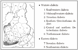
Traditional division of Finnish dialects (Savijärvi and Yli-Luukko, 1994).
We also use a second test corpus, a set of some 9,000 lexical distribution maps that were drawn as a part of the editing process for the Dictionary of Finnish Dialects (Tuomi, 1989). We have already performed some initial analyses of this same corpus (Hyvönen et al., 2007), and using it here makes it possible to build on the prior work. The main advantage, however, is that it is very different from the Dialect Atlas corpus. The Atlas corpus is much smaller but for the most part comprehensive, while the Dictionary corpus is significantly larger but contains a massive amount of noise, as different regions have been surveyed to widely varying degrees.
At this point we would also like to note that the methods we compare here are in no way specific to dialectological data but are instead general-purpose computational methods suitable for a wide range of multivariate analyses. We chose Finnish dialects as our test subject mainly because the corpora were readily available to us, and secondarily because of our prior knowledge of the field. Nevertheless, geographically distributed presence-absence data is common also in other disciplines, and the methods would be equally useful for analysing such variation.
2. Methods
According to the traditional view Finland is divided into separate dialect regions. The borders of these regions are commonly drawn along the borders of Finnish municipalities, since these were the basic geographical units used for collecting most of the original data. It is very natural to consider the data as a binary presence-absence matrix, with zeros indicating the absence and ones the presence of a feature in a municipality. It would therefore be attractive to apply clustering methods to our data sets and divide the municipalities of Finland into separate clusters, each corresponding to a particular dialect region. However, in reality dialect regions do not have sharp borders, and assigning each municipality to a particular cluster is not necessarily a good approach (Hyvönen et al., 2007).
An alternative is to use component methods to analyse the data. While we shall see later on that different methods do indeed perform differently, what all of the methods used in this study have in common is that they produce a small number of components that capture the most significant aspects of the overall variation. Because of this, the methods can also be thought of as latent variable methods: the components, or latent variables, capture the hidden structure of the data. For historical reasons different methods use different names to refer to these components, so that they are also called aspects or factors. In this paper, when we talk of latent variables or components or aspects or factors we are talking about the same thing, although strictly speaking we could make a distinction between the actual phenomena underlying the data and the components which are used to model them.
Ideally the components found are interpretable in terms of the dialect regions. We consider features as observations and municipalities as variables, and each element of a component corresponds to a municipality. Each component can be visualised as a choropleth map, with a colour slide between the extremes.
In mathematical terms we can express the data as follows:
D = FX (1)
where D is the data matrix, F contains our factors and X is the mixing matrix. If the factors in F correspond to dialect regions, the elements of X tell how these factors are combined to get the data matrix. One dialect word or feature is represented by one column in D, and the corresponding column of X tells how the k factors, stored in columns of F, combine to explain that dialect word.
2.1 Factor Analysis
Factor analysis (FA) aims to find a small set of factors which explain the data. For example, if solar radiation and temperature correlate strongly only one factor (‘sun’) can be used to explain them both. In our case, all Tavastian dialect features correlate strongly, so only one factor (‘Tavastian’) can be used to explain them. In other words, we would expect some correspondence between factors and dialects.
2.2 Non-negative matrix factorisation
Non-negative matrix factorisation (NMF) (Paatero, 1997; Lee and Seung, 1999) differs from factor analysis in that it aims to find non-negative factors which explain the data in a non-negative way. For example, a municipality in Kainuu could be explained using Savonian and Ostrobothnian components with weights 1 and 2 (‘this municipality is one part Savonian and 2 parts Ostrobothnian’). Similarly, a certain dialect word or feature could be half Tavastian and half southwestern.
In many applications non-negativity is intuitively appealing. For example, one of the classic tasks in exploratory data analysis is so-called market basket analysis, or finding regularities in the combinations of different items that customers buy during a single trip to a market. In this case, it is obvious that the original data is non-negative: one cannot easily have −2 cartons of milk. Dialectological data is also non-negative-a feature may not appear in a local dialect but its frequency cannot be negative. The same applies to factors extracted from dialect data, as it is very difficult to understand what it would mean to characterise a municipality as ‘−0.5 Tavastian’.
NMF forces all elements of both matrices on the right side in equation 1 to be non-negative. This means that in the ‘Tavastian’ factor the elements corresponding to Tavastian municipalities are positive, while elements corresponding distinctively non-Tavastian municipalities are zero. Similarly, if a dialect word is used in Savonia and Ostrobothnia, which are represented by two factors, then the elements of X in equation 1 corresponding to that word will be positive for the Savonian and Ostrobothnian factors and zero otherwise. It is thus possible to interpret these factors as approximating the relative weight of the different dialectal influences.
While the components are always non-negative there is no similar guarantee regarding the high end of the range. This is important if one wishes to compare the relative weights of the components; in such a case one must add a separate post-processing step to normalise the components.
2.3 Aspect bernoulli
The aspect Bernoulli (AB) method (Kaban et al., 2004) differs from the methods introduced previously in that it is designed for binary data. Moreover, interpretation can in this case be given in terms of probabilities, so that for instance a municipality (or dialect word or feature) is 83% Savonian. This makes the method attractive for our use.
The AB method is also designed to distinguish between false and true presence and absence in data, which means it is suitable for dealing with noisy data. This should be good news for dealing with the Dialect Dictionary data set, which has a very large number of false absences, as all municipalities have not been thoroughly sampled. However, it seems that too much is too much: the missing values in the data set, far from being randomly distributed, are a consequence of systematic differences in sampling frequencies, and AB did not deal well with this kind of missing data.
2.4 Independent Component Analysis
Independent Component Analysis (Ica) (Hyvärinen Et Al., 2001) is Typically Used To Separate Signals With Several Measurements and A Few Measuring Points. A Classical Problem Would Be the So-called Cocktail Party Problem: We Have Five Microphones In A Room With Five People Talking, and We Wish To Separate These Speech Signals. Here We Consider Dialect Words Or Features As the Signal, and By ‘monitoring’ This Signal In Each Municipality We Use Ica To Discover the the Source of Those Signals, I.e. the Dialects Themselves.
ICA aims to find factors, or in this context components, that are statistically independent. ICA uses PCA as a standard preprocessing step, so that the number of principal components used depends on the number of factors sought. In our study we only use a small number of the principal components, as otherwise the resulting components tend to be too localised.
2.5 Principal components analysis
Principal components analysis (PCA) (Hotelling, 1933) is the oldest and probably also the best known method used in this study. PCA finds the direction in the data which explains most of the variation in the data. This is the first principal component. After this each consecutive component explains the variation left in the data after the variation explained by previous components has been removed. Note that each component must be interpreted bearing the previous components in mind. The principal components, especially the first ones, give a global view of dialects, but in general the components do not directly correspond to individual dialect regions.
In all of the previous methods described the number of factors chosen is crucial: different choices give different components. If the number of components k is large, the components are more localised, whereas for small k we tend to get components which correspond to a rough partitioning of dialects. In contrast, no matter how many components are computed by PCA the first k components are always the same. The first principal component will alwayspresent the main direction of variation. Principal components will therefore in general not represent the different dialect regions per se, but instead they give a global view of the variation. For example in Figure 2 we see that in the Dialect Dictionary data, after east-west variation is accounted for the next most important factor is the north-south variation.
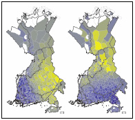
Dialect Dictionary, principal components 2 and 3. The first principal component (not shown) captures the sampling rate (Hyvönen et al., 2007). The second component captures east-west variation, with the western influence shown as the blue and the eastern influence the yellow end of the colour scale. Similarly, the third component shows the north-south variation as the most significant direction after the east-west variation has been removed.
In explaining the data PCA certainly does as well as the other methods, but unlike these it does not directly summarise the contributions of different dialects as the components. This is often done using rotation as a post-processing step, but the rotation of the first few principal components does result in something that should not strictly speaking be called principal components any more.
3. Comparison of the Methods
In order to compare the five different methods we have used each to divide both data sets into ten components, or in the case of PCA looked at the first ten components. In comparing the results we have used two criteria: spatial autocorrelation and the degree to which the components conform to the existing dialectological view.
It should be kept in mind that the traditional view of Finnish dialects is largely based on the material presented in the Dialect Atlas. Even though this has been supplemented by later research, the relationship is strong enough that the traditional view can be considered the primary criterion for comparing the methods, especially for the Dialect Atlas data. The correspondence is not perfect, as is easily seen from comparing the traditional division in Figure 1 to a nine-way aspect Bernoulli analysis in Figure 3, and with the Dialect Dictionary data this relationship is somewhat weaker still. Nevertheless, the traditional view is a useful yardstick for comparing the methods.
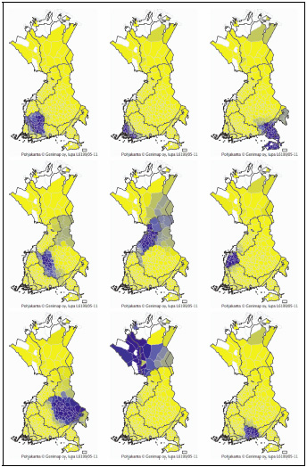
Nine distinct dialects as extracted by aspect Bernoulli from the Dialect Atlas data.
Measuring spatial autocorrelation shows essentially how cohesive each of the components is. When dealing with dialectal phenomena, it is reasonable to assume that the underlying phenomena do not have spatial discontinuities: in general, linguistic innovations spread across space in such a way that there are no major gaps within the resulting region. However, noise in data may result in noisy components. Using spatial autocorrelation as a quality measure favours methods which are more robust with respect to noise.
We use two different measures for autocorrelation. On the one hand, we use Moran's I statistic (Bailey and Gatrell, 1995:269–71):

Here n is the number of municipalities, wij is 1 where municipalities i and j are neighbours and 0 otherwise, yi is the value of the component in municipality i and Ӯ the average value of the component.
Values of I 〉 0 indicate that the value of the measured phenomenon tends to be similar in nearby locations, while I 〈 0 when the values at nearby locations tend to differ.
On the other hand, we also use Geary's C statistic (Bailey and Gatrell, 1995:270):
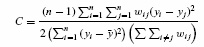
The C statistic shows the variance of the difference of neighbouring values, and thus tends to favour smaller-scale autocorrelation effects than the more globally oriented I statistic. The C statistic varies between 0 and 2, and values 〈 1 indicate positive autocorrelation.
To augment these two autocorrelation measures we use the correlation between a component and the closest traditional dialect region, as this gives some indication of how well these methods agree with more conventional dialectology. Correlations in the usual sense were calculated for a component and all the traditional regions over the municipalities, and the greatest of these correlations was chosen. Values between −1 and 0 indicate negative and those between 0 and 1 positive correlation.
Table 1 shows the summary of our results. It shows for each of the methods and data sets the average of the I and C statistics of the ten components; similarly, it shows the average of the correlation between each component and the closest-matching traditional dialect region. It is not possible to give absolute guidelines on which values are significant, as this depends very much on the properties of the original data, but in short the I statistic and the correlation should be as large and the C statistic as small as possible. To illustrate the differences between the methods, Figure 4 shows the component that corresponds most closely with the northern and central Tavastian dialects in the two corpora.
Table 1. Comparison of different analyses. For spatial autocorrelation, the column I should be 〉 0 and C 〈 1; for correlation between the analysis results and the traditional view of dialects, the column Dialect should be 〉 0.
| Atlas | Dictionary | |||||
|---|---|---|---|---|---|---|
I | C | Dialect | I | C | Dialect | |
FA | 0.88 | 0.12 | 0.75 | 0.74 | 0.30 | 0.59 |
NMF | 0.90 | 0.13 | 0.81 | 0.66 | 0.48 | 0.58 |
AB | 0.89 | 0.14 | 0.83 | 0.53 | 0.52 | 0.47 |
ICA | 0.93 | 0.07 | 0.60 | 0.71 | 0.41 | 0.50 |
PCA | 0.87 | 0.12 | 0.55 | 0.67 | 0.46 | 0.41 |
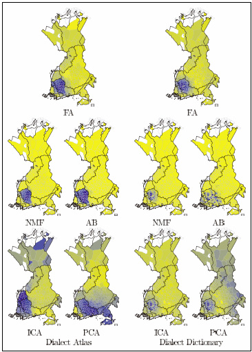
‘Northern Tavastia’ in the two data sets.
The maps derived from the Dialect Atlas in Figure 4 show how non-negative matrix factorisation and aspect Bernoulli give much more clearly defined dialects than the other methods. This is also reflected in Table 1: in the columns for the Dialect Atlas, both I and C show strong autocorrelation, and the components correlate highly with traditional dialect regions. However, the columns for the Dialect Dictionary in Figure 4 and Table 1 show that both methods are sensitive to noise in the data, so that in this case the components are spotty, with the least degree of autocorrelation among the five methods.
Independent component analysis has the strongest autocorrelation with the Dialect Atlas data and performs quite well also with the much more noisy Dialect Dictionary data. On the other hand, the components it discovers do not bear as much resemblance to the traditional dialectological understanding. This is especially apparent in the Dialect Atlas data, as evidenced by Figure 4; it is much less visible in the Dialect Dictionary data, where the other methods do not perform much better. In estimating the reliability of the components one should remember that the Dialect Atlas data set is relatively small, whereas ICA in general works better when the sample size is large.
Factor analysis performs reasonably well with the Dialect Atlas data: while it is not the best it still gives results that are both reasonably well autocorrelated and easily interpretable in dialectological terms. With the Dialect Dictionary data, however, it is the clear winner.
Finally, principal components analysis gives components that are spatially cohesive, with autocorrelation measures that are on par with the other methods. However, it is not very good in discovering dialects themselves-but that is because it does not attempt to do so. Instead, it finds directions of variation that are in a sense one step further, underlying the dialects themselves. This means that the first few components may give new insight, but very soon the further components become hard to interpret.
4. Comparison of the Corpora
It is also interesting to take the opportunity to look briefly at how the different corpora-one dealing largely with morphological and phonological, the other entirely with lexical variation-show a slightly different division of the Finnish dialects. The subdivision of the southwestern and southeastern dialects is particularly interesting.
As seen in Figure 5, factor analysis of the Dialect Atlas data finds both the traditional southwestern and mid-southwestern dialects as expected. The latter is usually considered a group of transitional dialects between the southwestern and Tavastian dialects, and its existence is explained by settlement history and trade routes in the middle ages. A similar analysis of the Dialect Dictionary data, however, divides the dialect into a northern and eastern group along the coastline, with the dividing line following the medieval highway from the coast inland. The contacts within each of these regions are still strong, and it is possible to view the difference between the two corpora as reflecting, in one case, Viking-age settlement and medieval contacts and, in the other, more modern cultural unity.
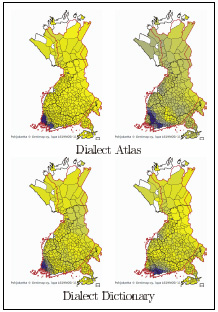
Division of the southwestern dialects given by factor analysis.
Figure 6 shows a similar division of the southeastern dialects. The Dialect Atlas gives the Carelian isthmus and the Finnish-speaking areas in Ingria as one group and the northwestern coasts of Lake Ladoga as the other. This is historically understandable, as Ingria was settled from Finland in the 17th century, after Sweden took the area from Russia; on the other hand, the northern coast of Lake Ladoga was historically bilingual between Finnish and the closely related Carelian. The Dialect Dictionary, however, divides the dialect along the pre-World War II border between Finland and Russia.
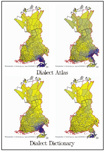
Division of the southeastern dialects given by factor analysis.
In both cases the differences seem to stem from the differences in how grammatical and lexical features spread. Words are easily borrowed from neighbours, so lexical data divides these two regions along the lines where people had most contact-in the case of southwestern dialects from the late medieval or early modern period onwards, in the case of southeastern dialects since the pre-WWII borders were established in the early 19th century. The morphological and phonological features, however, reflect a significantly older contact, and in this case it is even plausible to consider that the differing features did not spread by borrowing from neighbours but instead by the people themselves moving.
5. Conclusions
There are several component analysis methods that can be used to analyse corpora of isogloss or other presence-absence data. Such data exists in a wide range of disciplines, from archaeology to zoology; from a methodological point of view it is rather arbitrary and even irrelevant that we have chosen dialectal variation as our subject. The methods are all useful, but each has its own limitations, and these limitations should be kept in mind when selecting the method for a particular dialectological task. Similarly, the properties of the chosen method are relevant when interpreting the results.
The oldest of the methods in this study, principal components analysis, can be useful for trying to get one step beyond the dialect division itself: the components it finds should not be viewed as separate dialects but rather as a layered view of the variation. In interpreting each of the components one should always keep in mind that the bulk of the variation has already been explained away by the earlier components. This makes interpretation hard.
Although almost as old as PCA, factor analysis is still one of the most useful methods here. In fact, a large part of this study can be summarised as a general guideline: ‘if in doubt, start with factor analysis’. This method may not be the best, but in analysing the two quite different corpora it gave solid and easily interpretable results in both cases.
Turning to the more recent methods, Independent component analysis may be useful for giving a fresh look into the variation, especially if there is a large amount of data. In the present case, its results have less resemblance with traditional dialectological notions, and in some cases such new insight can be useful. For a more mainstream view of the dialect variation, however, the other methods would likely be more useful.
With the last two methods, Non-negative matrix factorisation and aspect Bernoulli, one of the key questions is the amount of noise in the data. These two seem to be the most sensitive to the effects of uneven gathering of the raw data. On the other hand, when the data results from a survey that has treated the whole study area with equal thoroughness, these methods give very good results.
Finally, the two corpora we used were different in that one consists mostly of grammatical and the other of lexical features. This difference is reflected in the results, so that while analysis of both corpora shows mostly quite similar dialects there are also differences. These differences can be explained by the different ways that lexical and grammatical innovations spread: in short-and getting dangerously close to oversimplifying-lexical elements are transferred via cultural contacts, while morphological and phonological features seem to spread most easily when the speakers of a dialect themselves move to a new area. In the future it would be interesting to do a more thorough study of these differences, and also to compare dialects to the distributions of place names (e.g. Leino, 2007) or ethnological features (e.g. Vuorela, 1976).
References
Lee and H. Seung (
A. Leino (
| Month: | Total Views: |
|---|---|
| September 2023 | 3 |
| August 2024 | 1 |
| December 2024 | 1 |