


Abstract
Noise represents a threat to human and wildlife health, triggering physiological and behavioral challenges to individuals living close to sources of extreme noise. Here, we considered airport environments as sources of potentially stressful stimuli for birds and tested if those living near airports are under higher physiological stress than birds living in quiet sites. We used measurements of CORT in feathers (CORTf) as a proxy of chronic stress. We evaluated 14 passerine and 1 non-passerine species, living near three Brazilian airports. We found that, across species, individuals with a better body condition had lower CORTf concentration. At the species level, we found that CORTf concentration was not consistently affected by airport noise. Comparing individuals living in quiet sites with those living near airports, we found that 2 species had higher and 2 had lower CORTf concentrations near airports, while 11 species presented no significant differences between sites. At the population level, model selection indicated that the direction and strength of these differences are weakly related to species’ song frequency (peak frequency), as lower-frequency singers tended to present higher CORTf levels at airport-affected sites. In summary, we were unable to find a consistent response among species, probably due to species-specific differences in their response to anthropogenic disturbances. Instead, we found that species might be affected differently according to their singing spectral frequency and that individuals in good body condition show lower CORTf, suggesting that this measure is consistent with lower physiological stress.
Introduction
Humans have not only dramatically modified the Earth’s landscapes in the past centuries but also significantly increased the levels of pollutants in the environment, endangering the welfare of both wildlife and people (Jarrige and Le Roux, 2020). In addition to chemical pollution, noise pollution is now recognized as a problematic aspect of anthropogenic development, attracting increased attention in the past decades (Shannon et al., 2016). Noise pollution is known to influence aspects of wildlife behavior (Klett-Mingo et al., 2016), disrupt reproduction (Halfwerk et al., 2011) and change the dynamics of animal communities (Francis et al., 2009). These impacts demand further inquiry concerning which aspects of noise pollution affect wildlife, providing the knowledge for effective mitigation and management actions (Barber et al., 2009; Francis and Barber, 2013; Alquezar and Macedo, 2019).
Airport environments are affected by several disturbances, like extreme noise, air pollution, habitat degradation and habitat fragmentation, among others. Airports are a noticeable source of great amounts of noise, comprised by a wide spectrum of frequencies within the acoustic space at very high amplitude levels, jeopardizing the health and also communication among animals of different taxa (Gil et al., 2015; Alquezar and Macedo, 2019), including humans. Previous studies have shown that humans exposed to airport noise pollution face increased risk of hypertension, psychological and sleep disturbances, increased catecholamine secretion and impaired cognitive performance (Stansfeld and Matheson, 2003; Stansfeld et al., 2005; Jarup et al., 2008; Finegold, 2010; Floud et al., 2013).
Birds rely on vocal communication for the maintenance of social interactions (Hultsch and Todt, 1982; Catchpole and Slater, 2008) and noise can mask their most used song frequency bands (Wiley, 2013). Such masking can disrupt communication and reduce birds’ ability to perceive predators and to assess other risky situations (Quinn et al., 2006; Klett-Mingo et al., 2016), potentially inducing chronic stress (Kleist et al., 2018). In birds, airport noise has been associated to community homogenization (Alquezar et al., 2020b) and behavioral changes, such as vocal modifications (Gil et al., 2015; Dominoni et al., 2016; Sierro et al., 2017) and foraging disruption (Klett-Mingo et al., 2016).
Studies have suggested that, in urban environments, bird species are filtered based on their vocal characteristics (Francis et al., 2011), as lower-frequency singers avoid noisy environments (Gomes et al., 2021). Still, those species that remain in noisy areas might spend a greater amount of energy to maintain their vocal communication, either by increasing their song frequency and amplitude (Nemeth and Brumm, 2010) or by repeating their song more often in time (Sierro et al., 2017), creating a stressful condition. In this sense, it is expected that birds singing at lower frequencies would be more prone to stress in noisy environments. As well, it is expected that birds adapted to urban conditions (more common and abundant in cities) would be less prone to be stressed by noisy environments.
One way to evaluate how wildlife is responding to noisy environments created by urbanization is by measuring the levels of glucocorticoid hormones (Sapolsky et al., 2000; Romero, 2004) linked to the stress response. Long-term changes in these hormones may indicate whether a given population or an individual is chronically stressed (Dickens and Romero, 2013). The stress response can be defined as a set of behavioral and physiological changes that help an individual restore systemic homeostasis when exposed to noxious stimuli, such as predator exposure, shortage of food resources, competition and unfavorable climatic conditions, among other possibilities (Buchanan, 2000; Romero, 2004; Costantini, 2008; Dantzer et al., 2014). In birds, corticosterone (CORT) is the glucocorticoid hormone analogous to cortisol in mammals. When exposure to threats is occasional, CORT release induced by the hypothalamic–pituitary–adrenal (HPA) axis helps individuals to deal with risky situations (Wingfield and Kitaysky, 2002). However, when exposure to noxious stimuli is continuous, the stress response becomes chronic and can lead to detrimental consequences to the individual’s breeding activities, survival, and cognitive ability (Sapolsky et al., 2000; Kitaysky et al., 2003).
Animal responses to stressful conditions have been studied and reviewed by many authors, but the field has yet to achieve a consensus with respect to the expected direction of the physiological responses (see reviews: Breuner et al., 2008; Bonier et al., 2009; Busch and Hayward, 2009; Bonier, 2012; Dickens and Romero, 2013). Meta-analytical approaches show that chronic stress cannot be assessed by a single measure of CORT level, although, integrative measures (e.g. feather or fecal CORT) show a clearer pattern than hormone instantaneous measures (e.g. blood), in particular as a response to anthropogenic stress (Dickens and Romero, 2013). Recent studies show varying results, where vertebrates exposed to urban environments either present higher levels of plasmatic and fecal CORT (baseline only, instantaneous and integrated measures) (Dantzer et al., 2014) or no effects relative to baseline and stress-induced CORT levels (Iglesias-Carrasco et al., 2020). The latter study argues that the lack of detectable responses to urban habitats reflects the fact that most research has focused on the urban habitat per se, but not on the specific anthropogenic pressures that may affect wildlife in urban habitats (e.g. noise, light, air pollution, habitat quality).
Considering studies that have focused on the specific impacts of noise pollution on birds, evidence suggests that individuals from species that are common in cities (i.e. urban adapters or exploiters) are more likely to present no differences in baseline CORT levels and/or in body condition when compared to individuals of the same species in quiet areas (e.g. song sparrow, Melospiza melodia: Grunst et al., 2014; house sparrow, Passer domesticus: Angelier et al., 2016; and house wren, Troglodytes aedon: Davies et al., 2017). This lack of baseline CORT level differences can be either because the species is insensitive to these disturbances (Grunst et al., 2014; Angelier et al., 2016) or because the species have adapted to the stressful condition (Davies et al., 2017).
In the past decade, several techniques have been developed to extract and measure corticosterone levels in feathers (CORTf) (Bortolotti et al., 2008). CORTf is an integrated measure of the hormone levels, representing a long-term hormonal response by the HPA axis. It is less invasive than blood measurements, not influenced by instantaneous researcher-bird manipulation and is considered a useful technique for studies in avian stress physiology and conservation (Bortolotti et al., 2009b; Sheriff et al., 2011; Fairhurst et al., 2013; Dantzer et al., 2014; Romero and Fairhurst, 2016). Research has shown that plasmatic CORT metabolites are deposited in feathers during their annual growth, when feather structures are being irrigated by blood (Jenni-Eiermann et al., 2015). When feather growth ends, the keratinized tissue preserves the stored CORT (Bortolotti et al., 2008). Once feathers are collected and stored in museums and collections, the stored CORT levels remain stable for several years, resistant even to heat and freezing (Bortolotti et al., 2009a).
Using measurements of corticosterone in feathers (CORTf), in this study, we tested the main hypothesis that Neotropical birds living in the vicinity of airport environments are under higher physiological stress than those living in quiet environments. Due to a concern about whether CORTf (or baseline CORT) is an appropriate proxy of stress levels (Dickens and Romero, 2013), we first investigated whether an individual’s CORTf concentration is related to its Body Condition Index, given that body condition has been suggested as the best measure of chronic stress (Dickens and Romero, 2013).
At the species level, we tested whether differences in CORTf concentrations between the two types of areas (airport-affected and quiet control sites) follow the same general trend, or alternatively, are species-specific. At the population level, we tested whether song frequency and preference for urban environments could explain the direction and strength of the response. In this context, we predict that species with higher song frequency and stronger preference for urban environments would show a weaker CORTf response.
Materials and Methods
Study sites
We collected data in patches of native vegetation in the immediate surroundings of three airports in Brazil (airport-affected sites). For each airport-affected site, we selected a nearby quiet control site (8–17 km distant from the airport), with a similar vegetation structure (Fig. 1). Airports were selected based on their high aircraft activity and the availability of native vegetation around the lanes. Airport-affected and quiet control sites are located in three different regions of Brazil (Brasília, Campinas and Salvador), 790–1450 km apart from each other.
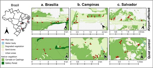
Location of study sites in Brazil, including airport-affected and quiet control sites for each studied region.
Characterization of study sites.
| BRASÍLIA | CAMPINAS | SALVADOR | ||||
|---|---|---|---|---|---|---|
| Airport | Control | Airport | Control | Airport | Control | |
| Landscape structure | ||||||
| % Native | 73.60 | 94.35 | 37.22 | 48.03 | 37.60 | 83.10 |
| % Degraded and urbanized | 26.40 | 5.65 | 62.78 | 51.97 | 62.40 | 16.90 |
| Noise levels | ||||||
| Minimum amplitude (dB) | 38 | 35 | 40 | 36 | 37 | 36 |
| Mean amplitude (dB) ± sd | 52 ± 8 | 38 ± 2 | 54 ± 8 | 41 ± 3 | 51 ± 8 | 43 ± 3 |
| Maximum amplitude (dB) | 86 | 54 | 92 | 60 | 92 | 70 |
Landscape structure: percentage of landscape classes within each study site. Noise levels: values of minimum, mean and maximum amplitudes (dB = decibels) for each study site, during sunrise time, in frequency range of 1–2 kHz (technophony). Table information adapted from Alquezar et al. (2020b).
The six study sites are identified according to whether they are an Airport (AIR) or a quiet control (CONT) site, and by the region/city where they are located (Brasília, Campinas or Salvador). At the Brasilia region (Distrito Federal) we selected the Presidente Juscelino Kubitschek International Airport (AIR_Bras: −15.872°, −47.919°) paired with a quiet control site, the “Parque Nacional de Brasília” (CONT_Bras: −15.728°, −47.951°). At the Campinas region (São Paulo state) we selected the Viracopos International Airport (AIR_Camp: −23.006°, −47.141°) and a private farm named “Fazenda Santa Maria” (CONT_Camp: −23.098°, −47.130°). And at the Salvador region (Bahia state) we selected the Luís Eduardo Magalhães International Airport (AIR_Sal: −12.916°, −38.338°) and a residential area with large and protected areas named “Condomínio Buscavida” (CONT_Sal: −12.859°, −38.270°).
In Alquezar et al. (2020b) we provide a characterization of each study site regarding landscape structure and noise levels (Table 1). These characteristics will be summarized here for better understanding, but detailed methodology must be consulted in the original publication. Landscape structure: each airport-affected site and its correspondent quiet control site contain similar vegetation structure (biome-wise), but airport-affected sites present higher proportions of degraded and urbanized landscapes than quiet control sites, while the latter had higher proportions of native landscape. Noise levels: we evaluated mean noise amplitude within 1–2 kHz frequency band, where most technophony is concentrated (Towsey et al., 2014). In all pairs of sites, noise levels are higher in airport-affected sites, the difference being higher in the Brasilia region and lower in the Salvador region.
Data collection
We mist-netted wild birds at all sites and collected two to three feathers from each individual’s tail. Captured birds were banded with numbered metal bands (provided by the Brazilian Banding National System- CEMAVE-SNA/ICMBio) and measured for body weight and tarsus, wing and tail lengths. Collected feathers were stored in identified paper bags for later analysis. All procedures were submitted to and approved by the University of Brasilia Ethics Committee (129 022/2015 CEUA UnB), by the Brazilian System of Authorization and Biodiversity Information (SISBIO 42578), by the Brazilian Banding National System (CEMAVE-SNA 3856) and by the Brazilian National System for Management of Genetic Patrimony and Associated Traditional Knowledge (SISGEN AAA265A).
Captures were conducted using 10 mist-nets, during 10 mornings at each site, opened for five hours during the morning. Additionally, we conducted directional captures using isolated nets and playback stimuli to attract birds (Fokidis et al., 2009) of specific species, to increase sample sizes, balancing the number of individuals captured in airport-affected and quiet control sites. In airports-affected sites, mist-nets were set at a maximum distance of 250 m from flight lanes, and in quiet control sites, they were set without restrictions. Both sites in each region were sampled in alternate weeks within each region’s avian breeding season. Brasilia’s region was sampled during October 2014 and November 2015; Campinas’s region, November–December 2014; and Salvador’s region, December 2015 to January 2016.
Most birds in Brazil molt their remiges and rectrices following their breeding period (Marini and Durães, 2001; Silveira and Marini, 2012). The breeding period is concentrated at the rainy season (around September to January) while molt is expected to occur in the end of the rainy season (after January). Considering our fieldwork period (breeding period), we expect that captured birds had molted their feathers in the previous year. Among the species included in the analysis, three are migrants (Elaenia chiriquensis, Myiarchus swainsoni and Volatinia jacarina). All these three migrant species are known to breed (Marini et al., 2012) and molt in central Brazil (Queiroz, 2008; Silveira and Marini, 2012), where they were sampled. Awareness of these molting patterns provided us with the certainty that collected feathers were molted at the study sites where these migratory birds were sampled (Brasília and Campinas).
Feathers were collected exclusively from adult birds, thus we presume they grew within the same annual time interval for each species. We did not consider possible differences related to sex, because the majority of analyzed species have no sexual dimorphism (exceptions are V. jacarina and Coryphospingus cucullatus).
Feather processing and CORTf analyses
Each feather was individually weighed and measured for length (excluding calamus), since both methods are used in the literature to calculate concentration in steroid immunoassays (see below). Afterward, feathers were cut into very small pieces (< 2 mm). For each sample, we used 1–3 feathers from the same individual, and this material was weighed to the nearest 0.001 g with a high precision balance. In cases where feathers from a single individual did not provide enough material to produce a reliable assay (V. jacarina, Coereba flaveola and some Troglodytes musculus), we pooled feathers from two to three individuals to compose a single sample (up to six feathers). Pooled samples were restricted to individuals from the same species from the same site.
Methanol-based hormone extraction (corticosterone metabolites) was conducted following Bortolotti’s protocol (Bortolotti et al., 2008, 2009a), including adjustments suggested by Lattin et al. (2011). The minced feather samples were placed in silanized glass tubes, to which we added 6 ml of methanol (HPLC gradient grade, Prolabo (VWR), PA, USA). The samples were then placed in a sonicating water bath at room temperature for 30 min, followed by incubation at 50°C overnight (18 hours) in a shaking water bath. We added an additional volume of 2 ml of methanol to the samples, which were vigorously vortexed for 10 min, and then separated the liquid from feathers using a disposable syringe and a plug of synthetic polyester fiber (0.45 μm) for filtration. The methanol extract was placed in a new silanized glass tube and evaporated in a fume hood using a stream of nitrogen. After complete evaporation, we added 300 μl of steroid free serum (DRG Instruments GmbH, Marburg, Germany), quickly centrifuged the samples, stored the new extracts in plastic tubes and froze them at −20°C for subsequent corticosterone metabolites analysis. Hereafter, corticosterone metabolites are referred as corticosterone (CORT).
We ran a corticosterone enzyme immunoassay (EIA) using a CORT specific kit (DRG Instruments GmbH, Marburg, Germany), and read the plates in a Biotek spectrophotometer (Biotek Instruments, Inc, Winooski, VT, USA). Absorbance was read at a wavelength of 450 nm. Samples were assayed in duplicates, and CORT concentration was averaged from the two samples after regression of the standard curve of each plate. Intra-assay variation was calculated as the mean variation between duplicates (8.7%), and inter-assay variation was calculated as the mean of mean variation between lower and higher control concentrations of each plate (12.1%). Linearity of serial dilutions of sample pools was adequate. Laboratory analyses were conducted in the Ecophysiology Lab of the Museo Nacional de Ciencias Naturales (Madrid, Spain), from September to November of 2016.
Most studies indicate that expressing hormone levels in terms of feather length is a more appropriate approach (Bortolotti et al., 2008, 2009a; Jenni-Eiermann et al., 2015), however, some studies still express hormone values in terms of feather mass (Koren et al., 2012; Lendvai et al., 2013). Based on our own tests, the CORT concentrations based on feather mass and length were highly and significantly correlated (see Supplementary Material A for results; linear regression: F2,593 = 1561, P < 0.001, r2 = 0.72, intercept = 4.58−16, slope = 0.851). Given the high correlation between the two measurements, we chose to present feather hormone values as a function of each sample’s added lengths of all feathers (pg mm−1), following previous literature (Bortolotti et al., 2009a; Lattin et al., 2011).
Analysis
All analyses were performed in R (R Core Development Team, 2022) and statistical significance was considered at P < 0.05. Variables were tested for normality, box-cox transformed and scaled. All model significance was calculated with a post-hoc analysis of deviance (type III). To run these analyses we used packages “lme4” (Bates et al., 2014), “car” (Fox and Weisberg, 2011), “MuMIn” (Barton, 2016) and “AID” (Asar et al., 2017), as well as RStudio interface (RStudio Team, 2020). For figures we used “ggplot2” (Wickham, 2016) and “sjPlot” (Lüdecke, 2020), as well as Inkscape (Inkscape Project, 2020) for graphic editing.
Body condition
A Body Condition Index was calculated for individuals for which we had CORTf and body measurements (body weight, tarsus, wing and tail length), comprising a dataset of 10 species and 308 samples. First, we summarized body size of each species using a principal component analysis (PCA) based on tarsus, wing and tail lengths. Then we ran a regression between body weight and body size (PCA’s first axis) and used the regression’s residuals as our Body Condition Index (Schulte-Hostedde et al., 2005). Using this dataset, we investigated whether an individual’s CORTf concentration is related to its Body Condition Index (data available in Supplementary Material B). Here, higher index values represent individuals with better body condition. Finally, we ran a linear mixed model (LMM) using CORTf concentration as response variable and Body Condition Index as predictor. As random effect we included species ID and plate ID.
Species’ responses
To understand species’ response to different site types (airport vs. control), we fitted an exploratory LMM (global model 1), using CORTf as the response variable. The site type (airport or control) and species ID (n = 15 species) were included as predictors, as well as their interaction. The variable Region was included as a covariate and Plate id as random effect. For this analysis we used the full dataset (n = 595). The LMM was followed by a post-hoc analysis of deviance (ANOVA).
Subsequently, we fitted models for each species to assess species-specific responses. Similarly to the previous model, we used CORTf as the response variable and Site type (airport or control) as the predictor. We fitted simple LMs when samples were in only one plate or LMMs when samples were in more than one plate. For species with data from more than one region, we added region as covariate when the inclusion of this variable reduced models’ Akaike’s Information Criteria (AIC). Analysis script and output are available as Supplementary Material C.
Population responses
To understand whether population trends in CORTf concentration can be explained by species´ characteristics, we ran a model selection using the variable CORTf effect-size as the response variable and region, song frequency and degree of urbanity as predictor variables (explained below). We used a dataset of 512 samples, comprising 14 species and 18 populations. Population was defined as a group of individuals of the same species, captured in the same region (BRAS, CAMP or SAL). The samples were chosen based on a minimum number of five samples per site. Given the exploratory character of this analysis, we used “dredge” function to summarize the best models, ranking them by increasing Akaike’s Information Criteria (AICc) and considering models within ΔAIC < 2. We also accessed variables’ significance. Analysis script and output are available as Supplementary Material D.
CORTf effect-size: For each population, we calculated CORTf effect-size as the standardized effect difference between CORTf concentration found in airport-affected and quiet control sites (i.e. Hedge’s d;Nakagawa and Cuthill, 2007). Positive effect sizes indicate higher CORTf concentration in the airport-affected site relative to quiet control sites and negative effect-sizes indicate lower CORTf concentration in airports-affected relative to quiet control sites (raw means and effect-sizes available in Supplementary Material D).
Song frequency Index: This index represents each species’ peak frequency corrected by body weight. Peak frequency is the frequency in which species concentrate most of the song energy, and differently from minimum frequency, this measure is less affected by noise masking. To obtain these values, we selected a minimum of five recordings of each species (RDA unpublished data) and used Raven Pro 1.5 (Center for Conservation Bioacoustics, 2019) to measure the acoustic parameters of a total of 20 songs from each species, using a FFT of 1024. All selected recordings are from quiet control sites. As species’ song frequency has been shown to be affected by species’ body size (Ryan and Brenowitz, 1985; Demery et al., 2021), we corrected our peak frequency values by mean species body weight measured in each studied region. To do so, we ran a regression between peak frequency and body weight and used the regression’s residuals as our Song Frequency Index (used values available in Supplementary Material D).
Degree of urbanity: The degree of association of each species to urban environments was represented by the degree of urbanity. This variable was calculated using eBird (eBird, 2017) citizen data and details are provided in Alquezar et al. (2020a). Here, positive values are associated with species that exhibit some degree of preference for urban habitats while negative values are associated with species that exhibit some degree of avoidance of urban environments (values available in Supplementary Material D).
Results
A total of 1187 individuals were captured and had their feathers collected in the six sampled sites, totaling 124 species. Due to the reduced sample size for some species, after fieldwork completion we decided to keep only those species that had at least five samples for each site type (AIR or CONT). Doing so, our analysis used data for 15 species, totaling 595 samples (raw data available in Supplementary Material B). The feather CORT concentrations (CORTf) varied from 0.76 pg mm-1 to 182.86 pg mm-1 (mean = 7.36 pg mm-1; sd = 12.14). The 15 species analyzed belong to one non-passerine order and seven passerine families, including suboscines (five species) and oscines (nine species). All species are reasonably common in urban environments.
The non-passerine species is the Swallow-tailed hummingbird (Eupetomena macroura, n = 17). The Passerines include Suboscines (suborder Tyrannii): sooty-fronted spinetail (Synallaxis frontalis, n = 25), plain-crested elaenia (E. cristata, n = 33), lesser elaenia (E. chiriquensis, n = 59), swainson’s flycatcher (M. swainsoni, n = 32), great kiskadee (Pitangus sulphuratus, n = 64); and Oscines (suborder Passeri): rufous- browed peppershrike (Cyclarhis gujanensis, n = 20), southern house wren (T. musculus, n = 67), pale-breasted thrush (Turdus leucomelas, n = 72), rufous-bellied thrush (Turdus rufiventris, n = 13), rufous-collared sparrow (Zonotrichia capensis, n = 25), sayaca tanager (Thraupis sayaca, n = 53), blue-black grassquit (V. jacarina, n = 62), red-crested finch (C. cucullatus, n = 30) and bananaquit (C. flaveola, n = 23 samples).
Body condition
Here we tested whether an individual’s CORTf concentration is related to its Body Condition Index. If CORTf reflects chronic stress levels suffered by birds, we could expect to find lower levels of CORTf in individuals with higher body condition (i.e. healthier individuals). Using a dataset of 10 species comprising 308 samples, we ran a mixed model with Species id and Plate id as random factors and Body Condition Index as a predictor. As expected, we found a significant association between individual’s CORTf concentration and Body Condition Index (LMM estimate: -0.155; X2 = 9.870; df = 1; P = 0.001): individuals with higher body condition showed decreased CORTf concentrations. The pattern is consistent for most species (Fig. 2).
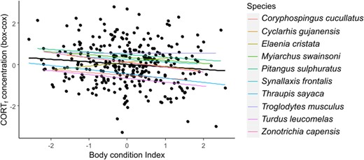
Relationship between CORTf concentration and Body Condition Index. Colored lines indicate each species pattern and black line indicates model pattern.
Species’ responses
For the species response analysis, we used a dataset of 15 species comprising 595 samples. We addressed the question of whether there was a consistent difference in CORTf concentration between birds in airport-affected vs. quiet control sites, and if this difference existed, whether it varied depending on the species. We found a significant interaction between site type (airport vs. control) and species ID (post-hoc Anova: P < 0.001), indicating that differences in CORTf concentration depend on species-specific differences and site types. Analyses also indicated a significant difference between regions (post-hoc Anova: P < 0.001).
In the species-specific models, two species presented significant increased CORTf concentration, and two species presented reduced CORTf concentration in the airport-affected sites (Fig. 3), compared to the quiet control sites. The rufous-browed peppershrike (C. gujanensis; P = 0.01) and the red-crested finch (C. cucullatus; P = 0.02) presented CORTf increases. The southern house wren (T. musculus; P = 0.02) and the bananaquit (C. flaveola; P = 0.01) presented decreases in CORTf in the airport-affected sites. The remaining species presented no significant changes in CORTf concentration between airport-affected and quiet control sites (Tables 2 and 3).

Species and site type interaction from species-specific analyses. Black circles represent outliers. The boxes show the median, interquartile range, and whiskers (indicating the 90th and 10th percentiles) for each species.
Species-specific models (LMs), for five species that were analyzed in a single plate, thus have no random effect included.
| CORTf concentration (pg mm−1) | ||||||||
|---|---|---|---|---|---|---|---|---|
| Estimate | SE | t value | P value | Airport | N | Control | N | |
| E. macroura (SAL) | ||||||||
| Intercept | 0.220 | 0.35 | 0.617 | 0.546 | 3.14 ± 0.5 | 9 | 3.47 ± 0.8 | 8 |
| Site type-airport | −0.415 | 0.49 | −0.848 | 0.410 | ||||
| S. frontalis (BRAS and CAMP) | ||||||||
| Intercept | −0.539 | 0.36 | −1.487 | 0.151 | 8.03 ± 5.3 | 18 | 4.18 ± 0.7 | 7 |
| Site type-airport | 0.749 | 0.42 | 1.753 | 0.093 | ||||
| M. swainsoni (BRAS and CAMP) | ||||||||
| Intercept | 0.0586 | 0.21 | 0.270 | 0.789 | 6.93 ± 2.7 | 10 | 8.39 ± 5.0 | 22 |
| Site type-airport | −0.186 | 0.38 | −0.483 | 0.633 | ||||
| Z. capensis (BRAS and CAMP) | ||||||||
| Intercept | 0.012 | 0.24 | 0.049 | 0.962 | 8.65 ± 9.1 | 8 | 7.16 ± 4.9 | 17 |
| Site type-airport | −0.037 | 0.43 | −0.086 | 0.932 | ||||
| T. rufiventris (ALL) | ||||||||
| Intercept | −0.404 | 0.31 | −1.296 | 0.221 | 5.99 ± 1.5 | 5 | 4.68 ± 0.9 | 8 |
| Site type-airport | 1.052 | 0.50 | 2.089 | 0.060 |
Raw means of CORTf concentration and sample size (N) in airport-affected and quiet control sites included. Models include only site type as predictor. Model’s statistics = t student. Complete model’s output available as Supplementary Material D.
Species-specific models (LMMs), for 10 species that were analyzed in multiple plates, thus have random effect included.
| CORTf concentration (pg mm-1) | |||||||||
|---|---|---|---|---|---|---|---|---|---|
| Estimate | SE | X2 | df | P value | Airport | N | Control | N | |
| CORTf ~ site type + (1|plate id) | |||||||||
| E. cristata (BRAS) | |||||||||
| Intercept | 0.161 | 0.32 | 0.242 | 1 | 0.622 | 5.99 ± 3.3 | 16 | 7.67 ± 4.3 | 17 |
| Site type-airport | −0.456 | 0.34 | 1.753 | 1 | 0.185 | ||||
| E. chiriquensis (BRAS) | |||||||||
| Intercept | −0.375 | 0.39 | 0.914 | 1 | 0.339 | 5.90 ± 3.5 | 22 | 3.92 ± 2.1 | 37 |
| Site type-airport | 0.583 | 0.38 | 2.353 | 1 | 0.125 | ||||
| C. flaveola (SAL) | |||||||||
| Intercept | 0.616 | 0.66 | 0.863 | 1 | 0.352 | 1.66 ± 0.6 | 9 | 2.17 ± 0.5 | 14 |
| Site type-airport | −0.944 | 0.39 | 5.811 | 1 | 0.015 | ||||
| T. sayaca (CAMP and SAL) | |||||||||
| Intercept | 0.280 | 0.20 | 1.793 | 1 | 0.180 | 3.92 ± 1.0 | 31 | 5.44 ± 2.9 | 22 |
| Site type-airport | −0.478 | 0.27 | 3.065 | 1 | 0.079 | ||||
| V. jacarina (BRAS and CAMP) | |||||||||
| Intercept | −0.345 | 0.29 | 1.345 | 1 | 0.246 | 3.97 ± 1.4 | 48 | 2.52 ± 1.1 | 14 |
| Site type-airport | 0.484 | 0.30 | 2.583 | 1 | 0.108 | ||||
| C. gujanensis (ALL) | |||||||||
| Intercept | −0.249 | 0.49 | - | - | - | 15.55 ± 11.4 | 10 | 6.46 ± 4.3 | 10 |
| Site type-airport | 0.937 | 0.38 | 5.807 | 1 | 0.015 | ||||
| P. sulphuratus (ALL) | |||||||||
| Intercept | −0.175 | 0.43 | 0.161 | 1 | 0.687 | 12.44 ± 12.7 | 54 | 9.11 ± 4.9 | 10 |
| Site type-airport | 0.121 | 0.35 | 0.121 | 1 | 0.727 | ||||
| CORTf ~ site type + region + (1|plate ID) | |||||||||
| T. musculus (ALL) | |||||||||
| Intercept | 1.105 | 0.19 | - | - | - | 13.64 ± 24.3 | 35 | 23.27 ± 34.7 | 32 |
| Site type-airport | −0.420 | 0.18 | 4.937 | 1 | 0.026 | ||||
| Region-CAMP | −1.047 | 0.23 | 41.648 | 2 | <0.001 | ||||
| Region-SAL | −1.508 | 0.23 | |||||||
| T. leucomelas (ALL) | |||||||||
| Intercept | 0.701 | 0.43 | - | - | - | 4.983 ± 3.35 | 41 | 4.19 ± 2.6 | 31 |
| Site type-airport | 0.178 | 0.27 | 0.405 | 1 | 0.524 | ||||
| Region-CAMP | −1.231 | 0.46 | 9.473 | 2 | 0.008 | ||||
| Region-SAL | −1.133 | 0.37 | |||||||
| C. cucullatus (BRAS and CAMP) | |||||||||
| Intercept | 1.135 | 1.22 | - | - | - | 4.77 ± 2.0 | 20 | 3.73 ± 1.7 | 10 |
| Site type-airport | 0.984 | 0.43 | 5.071 | 1 | 0.024 | ||||
| Region-CAMP | −0.823 | 0.55 | 2.202 | 1 | 0.137 |
Raw means of CORTf concentration and sample size (N) in airport-affected and quiet control sites included. Models include site type as predictor and region as covariate when the inclusion of this variable reduced models’ AIC. Model’s statistics = Chi-squared. Complete model’s output available as Supplementary Material D.
It is worth mentioning that the southern house wren (T. musculus), the pale-breasted thrush (T. leucomelas) and the red-crested finch (C. cucullatus), maintained region as an important variable after AIC comparison. However, region was considered significant for the southern house wren (P < 0.001) and the pale-breasted thrush (P = 0.008), but not for the red-crested finch (P = 013).
Population’s responses
Given the disparity of responses to Site type in CORTf concentration, we explored whether these differences between populations are affected by region, Song frequency Index and degree of urbanity. To this end, we applied a meta-analytical approach, using the effect-sizes of our dataset of 18 populations (14 species) comprising 512 samples. Model selection was run based on a full LM model resulting in the selection of two models (∆AIC < 2), the first including Song Frequency Index whereas the second option was the null model (Table 4). The general trend shows that species with a lower Song Frequency Index presented greater positive differences in CORTf concentration, with a higher CORTf concentration in airport-affected sites compared with quiet control sites (Fig. 4). Although Song Frequency Index was kept in the model, this variable was close to significance but not significant for the averaged model (P = 0.07). Degree of urbanity was not kept in the model as a useful predictor of CORTf differences between sites.
Model selection results for CORTf effect-size (population’s response).
| LM full model: CORTf effect size~ Region + Song frequency + Degree of urbanity | ||||
|---|---|---|---|---|
| Selected models | df | AICc | ∆AIC | Weight |
| Song frequency | 3 | 16.3 | 0.00 | 0.457 |
| Null | 2 | 17.1 | 0.76 | 0.312 |
| Song frequency + degree of urbanity | 4 | 19.4 | 3.05 | 0.099 |
Only models with ∆AIC < 2 were considered suitable.
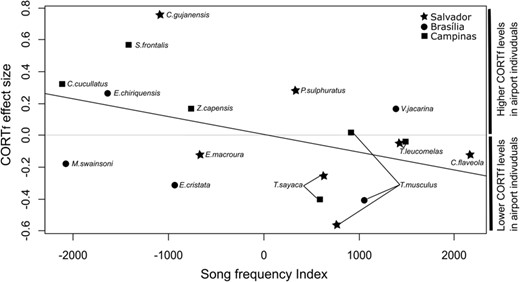
CORTf effect-size and Song frequency Index relationship from population’s response model.
Discussion
Stress induced by noise has been investigated in recent years for a few bird species, but results are not congruent, although Injaian et al. (2020) indicated that urban avoiders are potentially more sensitive to noise. Here, we evaluated corticosterone deposited in feathers as a long-term measure of the stress response in 15 bird species living in Brazilian airport-affected and quiet control sites. We considered that airport environments exhibit several disturbances, with noise as the most extreme and which is absent in other disturbed landscapes. First, we found that individuals with better Body Condition showed lower CORTf concentration; we can thus consider body condition as a good predictor of CORTf. Second, we found that species’ responses were not consistently affected by airport noise, although four species showed either higher or lower CORTf concentration in the airport-affected sites. At the population level, there was a weak indication that species with lower Song Frequency present higher CORTf concentration in airport-affected sites.
Body condition has been used as an index of an individual’s quality and reproductive success (Milenkaya et al., 2015; Montreuil-Spencer et al., 2019). Here, we evaluated whether CORTf concentration is related to Body Condition Index in our studied individuals, considering that feathers were grown in the previous 12 months, but the noxious impact of the airport environment is similar between years. The relationship found indicates that individuals with a better body condition (healthier) have lower CORTf levels, that is, birds that experienced lower circulating CORT during feather growth were in better body condition at the time of capture. It is important to observe that feathers were molted in the year before and are expected to be molted again within 1–2 months after data collection. Thus, we are assuming that the stressful environment (chronic stress) is repeatable in time and affects birds throughout their lives, not leading to great changes in the bird’s season-specific body condition.
This finding agrees with a study that associates body condition with baseline and stress-induced levels of plasmatic CORT in kittiwakes Rissa tridactyla (Kitaysky et al., 1999); as well as a study that associates body condition with feather CORT levels in tree swallows (Tachyneta bicolor) (Harms et al., 2010). A meta-analysis about chronic stress found that the best physiological predictor of chronic stress of any kind, both in experimental and correlative studies, is body mass (Dickens and Romero, 2013), which typically decreases when animals are subjected to chronic stress. Given that CORTf is an integrative measure that lasts long after the stress has been experienced, we can only rely on it to evaluate a stressful situation experienced during feather growth. It is necessary to be aware that the relationship between chronic stress vs. body condition and acute stress vs. body condition must be different because the information stored in feathers is relative to a restricted period of time. In this way, our results lend support to the use of CORTf as a reliable index of chronic stress (when noxious stimuli are continuously present).
Species-specific responses were highly variable. We found 2 species with higher CORTf concentration in the airport-affected sites, 2 species with lower CORTf concentration in the airport-affected sites and 11 species presenting no differences between airport-affected and quiet control sites. Species-specific responses to noisy environments can vary greatly (Francis and Barber, 2013), presenting a difficult and additional obstacle to establishing an expected physiological response to acoustic disturbance. The observed increased CORTf concentration in birds living near airports is easier to understand, since CORTf levels represent the accumulation of stress responses during the timeframe of feather growth and increased levels of this hormone is a typical response to noise reported for birds, fishes, and humans (Evans et al., 2001; Anderson et al., 2011; Crino et al., 2011; Strasser and Heath, 2013). This increased hormone level is classified as a stage of homeostatic overload by Romero et al. (2009), representing changes that exceed the normal reactive scope and cause physiological disruption (chronic stress). This overload can result in greater individual susceptibility to parasite infections (Bortolotti et al., 2009b) and decreased survival in the wild (Koren et al., 2012).
On the other hand, decreases in CORT concentration are less commonly reported in the literature, but according to Romero et al. (2009), this may be observed in individuals experiencing homeostatic failure. This is a more severe state of chronic stress, representing changes that cause physiological disruption and death, with hormone levels below the predictive homeostasis range, which has also been shown to be related to lower reproductive success (Kleist et al., 2018). Reductions in basal and stress-induced plasmatic CORT levels have been reported for captive and free-living birds (Rich and Romero, 2005; Cyr et al., 2007; Cyr and Romero, 2007), and these changes were associated with reduced body weight and lower fledging success. The authors discarded the possibility that these results could be due to habituation to the stressor and exhaustion, and claimed that the response must be a controlled systemic downregulation of HPA activity (Rich and Romero, 2005). Explanations relative to reduced baseline CORT levels observed for other taxa include (1) acclimation to a repeated stressor, (2) a real reduction of stress conditions due to higher resource availability or (3) a state of chronic stress (French et al., 2008). Considering the biology of species that presented decreased CORTf here, both are very small birds, highly abundant in urban environments in Brazil. Due to the small population size found for T. musculus in all three studied airports, we speculate that this species is not dealing well with the airport condition and might be in a chronic stress state.
For the remaining 11 species that presented no changes in CORTf concentration, we speculate that they are habituated to noisy conditions. Based on the possible explanations for either increased or reduced levels of CORTf concentration, we assume that CORTf levels must be influenced by factors other than only extreme noise, and that species are not consistently affected by noise in the same way. We highlight the fact that the analyzed species are reasonably common in urban environments since they are able to live in airport environments and deal with the associated environmental degradation. We emphasize that these results should be taken cautiously when considering species that are more sensitive to urban environments. Species that are of conservation concern such as the northern spotted owl (Strix occidentalis caurina) (Hayward et al., 2011) and the greater sage-grouse (Centrocercus urophasianus), can be severely affected by noise, as shown in noise playback experiments (Blickley et al., 2012).
When evaluating population aspects that could explain the species-specific responses, we expected that species with lower song frequency would be more affected by noise due to frequency masking and jeopardized communication (Gil and Brumm, 2014). Our model selection showed that Song Frequency Index (peak frequency corrected by body weight) is a potential explanation for increased hormonal responses observed in airport-affected sites, denoting that species that vocalize in lower frequencies are more prone to being physiologically stressed in airport-affected sites. Although the relationship that we found is neither strong nor significant, it is in accordance with previous studies showing that anthropogenic noise filters out bird species that have low song frequencies (Francis et al., 2011; Proppe et al., 2013; Cardoso, 2014). Species that vocalize at lower frequencies may be burdened in noisy environments, having to shift their song frequency (Luther et al., 2016), increase their vocal amplitude (Schuster et al., 2012), and even avoid noisier areas (McClure et al., 2013, 2017; Proppe et al., 2013). We also expected that species that exhibit a preference for urban habitats would be less affected by noise (Injaian et al., 2020). However, this variable was not included in the selected models, probably because the analyzed species do not show great differences related to urban sensitivity.
The four species that presented increased or decreased CORTf levels in the species-specific analysis belong to the suborder Passeri (known as oscines or songbirds). The oscines produce more complex songs than suboscines. They have a more complex syringe, learn their songs, have a more diverse repertoire and higher ability to modify their songs (Catchpole and Slater, 2008). This phylogenetic similarity in the species that presented some degree of hormonal response to airport environments, allow us to speculate that oscine birds might be more affected by this environmental disturbance (noise). In the same way that population-specific analysis indicated a possible relationship between CORTf levels and song frequency, it is possible that song complexity might be an important variable to define which birds have their CORT levels affected by noise (Ríos-Chelén et al., 2012). This aspect should be tested by future studies.
In summary, our study shows that CORTf concentration and Body Condition Index are related, providing support to the idea that this integrative measurement can be used as a proxy to assess chronic stress in birds. We also show that birds living in the proximity of airports do not exhibit consistent elevations of CORTf in their feathers, but that species with low frequency songs seems be more affected than those with higher song frequency. Although extreme noise seems to be the factor driving such responses, it is important to notice other probable aspects of airport environments that could be affecting CORTf concentration (e.g. air pollution, nearby urbanization, resource availability, etc.). We stress that these results should be taken with caution when considering species that are more sensitive to urban environments, since our analyses only comprise less sensitive species.
Acknowledgements
We thank all field assistants for help with data collection, INFRAERO, INFRAMÉRICA, Brasil Aeroportos and Brazilian Air Force for allowing fieldwork within airport surroundings, IBAMA/ICMBio for permits to work in Brasilia National Park, and landowners for allowing access to their land.
Author Contributions statement
Study conception, resource acquisition and project supervision: D.G. and R.H.M.; data collection, statistical analysis and results interpretation: R.D.A. and D.G.; laboratorial analysis: R.D.A., L.A. and D.G.; draft manuscript preparation and figures: R.D.A. All authors reviewed the results and approved the final version of the manuscript.
Conflicts of Interest
The authors have no conflicts of interest to declare.
Funding
This work was supported by the Brazilian National Council for Scientific and Technological Development (Conselho Nacional de Desenvolvimento Científico e Tecnológico-CNPq), as part of the “Ciências sem Fronteiras” project, type “Visiting Researcher” [grant number 406911/2013-4]. D.G. was supported by funds from a research grant [grant number CGL2014-55577-R] from the Spanish Ministry of Science. RHM received a fellowship from CNPq for the duration of the study. R.D.A. was supported by scholarships from both CNPq and CAPES (Coordenação de Aperfeiçoamento de Pessoal de Nível Superior).
Data Availability
The data underlying this article are available in the article and in its online supplementary material.
