


Abstract
This article analyses the effects of financialisation on non-financial companies’ (NFCs) investment and explores the interactions between financialisation and the structural and institutional features of developing and emerging economies (DEEs). We estimate the effects of financialisation on physical investment for a sample of DEEs using panel data based on the balance sheets of publicly listed NFCs. Our main contribution is to assess the interactions between the financialisation of the NFCs and country-level financial development, financial reform, capital account openness and global value chain participation. We find that the effects of the financialisation of the NFCs in DEEs are highly context specific. Stock market development, financial reforms for liberalisation, capital account openness and participation in the global value chains are associated with more pronounced negative effects of financialisation on investment. Our analysis provides novel empirical evidence regarding the sources of variation in the financialisation of corporations in DEEs.
1. Introduction
The last decades have witnessed ‘financialisation’ as a central phenomenon in the evolution of economies. Financialisation has been summarised as an ongoing and self-reinforcing economic and social process that manifests itself in the growing prominence and influence of behaviours derived from the financial sector (Epstein, 2005). Van der Zwan (2014) highlights three main features of this process: (i) a new regime of accumulation largely shaped around financial motives, (ii) the consolidation of the ‘shareholder value’ as the key principle in corporate governance and (iii) rising influence of finance within everyday life (pension schemes, mortgages, healthcare etc.). This article aims at analysing the impact of financialisation on investment in the context of developing and emerging economies (DEEs) with a focus on the first two aspects.
Despite a growing theoretical literature on the effects of financialisation on physical investment, the empirical analysis is mainly focused on developed countries. However, ‘the growing influence of financial markets and institutions, known as “financialization”, affects how wealth is produced and distributed’ (UNCTAD, 2015, p. 27) also in the context of DEEs. Demir (2007, 2009) analyse the negative impacts of financialisation on investment taking into account financial liberalisation for a set of emerging countries, while Seo et al. (2012) provide similar evidence about Korean non-financial corporations’ (NFCs) Research and Development (R&D) investments. Hecht (2014) presents a comparative analysis of the effects of financialisation on the NFCs in advanced and large developing economies, also testing competing heterodox theories on the effects of financialisation on investment.
In the development literature, the effect of financialisation on uneven international development has been highlighted (Becker et al., 2010; Bonizzi, 2013). Karwowski and Stockhammer (2016) compare macroeconomic aspects of financialisation (e.g. financial deregulation, financial inflows, business and household debt levels) in emerging economies and find a considerable degree of variability in the intensity of financialisation, in line with the ‘varieties of financialisation’ observed across the developed countries (Lapavitsas and Powell, 2013; Karwowski et al., 2019). Bonizzi et al. (2020, 2022) highlight the subordinate position of DEEs within the global hierarchy of financial and production relations, which shapes and consolidate different forms of financialisation in DEEs, ultimately benefiting the top of the pyramid in which developed country multinationals can consolidate their dominant position.
This paper contributes to the literature on the financialisation of the DEEs’ NFCs by shedding light on the under-analysed specific forms of financialisation in the emerging capitalist countries, considering the key aspects of financial liberalisation and the hierarchical nature of international production relations. The aim is to provide an empirical substantiation to the claims of the variegated/subordinate financialisation literature with a focus on the financialisation of the NFCs, in particular by analysing the relations between financial and productive subordination.
Our analysis builds on and integrates these two strands of literature in two aspects by providing (i) micro-econometric evidence on the effects of financialisation on investment using firm-level data for a fairly comprehensive sample of DEEs and (ii) a variegated analysis of the interaction of the structural and institutional features of the country and the process of financialisation.
We confirm the negative effects of financialisation on investment for a comprehensive sample of DEEs, and we identify the key dimensions along which this relationship differs across countries. Our results suggest a significant interaction between country-level structural and institutional features and firm-level financialisation. Although at the aggregate level the negative effects of financialisation on investment in DEEs are similar to what has been found for developed countries (although with some differences), our disaggregated analyses point to novel findings. We find that both higher degrees of financial liberalisation and stronger stock market development are associated with significant negative effects of financialisation. Similarly, a higher degree of capital account openness is associated with stronger negative effects of financialisation on the NFCs’ investment. In addition, the investment of NFCs in countries that are relatively more integrated within the Global Value Chain (GVC) suffers more from an overall negative effect of firm-level financialisation. Our results provide useful insights for policy debates regarding the role and capacity of the DEEs’ governments to mitigate the effects of national and regional processes of financialisation on investment.
The rest of the article is organised as follows. Section 2 reviews the literature on the financialisation of investment with a focus on DEEs. Section 3 presents our econometric model. Section 4 introduces the data, key stylised facts, and the estimation methodology. Section 5 discusses the estimation results. Section 6 concludes.
2. Investment, financialisation and development
From a mainstream perspective, the liberalisation and growth of financial markets are expected to facilitate the financing and efficient allocation of investment (Beck et al., 2000; Beck and Levine, 2004; Love, 2003; Levine, 2005).
However, post-Keynesian research highlight the negative impacts of an expanding financial sector on income distribution and demand (Onaran et al., 2010; Hein, 2015), and in particular on investment, providing evidence that increasing engagement of the NFCs with financial markets in the developed countries has decreased their investment (Stockhammer, 2004; Orhangazi, 2008; Cordonnier and Van de Velde, 2015; Davis, 2018; Tori and Onaran, 2018, 2020, among others).
The financialisation of the NFCs is a phenomenon that became evident also in the context of developing countries. In the last decades, there has been a general decline in investment as a ratio to profits, and an increase in dividends as a ratio to profits, financial assets as a ratio to total assets and debt ratios (UNCTAD, 2016). Regarding DEEs, Demir (2007, 2009) finds that financial liberalisation in Argentina, Mexico and Turkey channelled savings from the productive sector towards financial speculation, thus reducing the availability of funds for long-term physical investment and increasing returns on financial assets relative to fixed assets, significantly reduced investment in these emerging market NFCs.
The literature suggests the effects of financialisation depend on the specific institutional context. In this work, we consider various potential institutional factors mediating the effects of financialisation on investment in the context of DEEs following Akkemik and Ozen (2014).
Even though the available evidence depicts financialisation as a phenomenon common to both advanced and developing economies, the different institutional settings at the country and/or regional level reveal the presence of ‘varieties of financialisation’ (see Dore, 2008; Pike and Pollard, 2010; Lapavitsas and Powell, 2013). Moreover, some recent contributions put forward an interpretation of the financialisation process at the global level showing that emerging economies are in a subordinate position with respect to advanced countries, with the latter dominating both the production and financial spheres (Bortz and Kaltenbrunner, 2018; Bonizzi et al., 2020, 2022).
In this paper, we analyse three channels of interaction between the macroeconomic institutional features of DEEs and the financialisation of the NFCs. Our main interest is to explore the associations between country-level macroeconomic institutional features and firm-level investment behaviour in the context of financialisation.
First, we test whether a more developed financial sector reinforces the impact of financialisation on investment in the context of DEEs. The mainstream literature argues that firms with higher financing obstacles experience slower growth, but this relationship is weaker in countries with relatively more developed financial systems, and financial development is more effective in alleviating financing constraints, especially for smaller firms (Beck et al., 2005). However, while some studies find a significant and positive effect of financial development on economic growth and investment (Love, 2003; Hermes and Lensink, 2003; Levine, 2005), both the statistical significance and size of the estimates vary widely due to methodological heterogeneity (Valickova et al., 2015). Alternatively, Tori and Onaran (2020), focusing on European countries, find that the negative effect of financialisation on NFCs’ investment is stronger in countries with a relatively high level of financial development. We assess whether higher levels of activities in the financial markets and intermediaries delinked from the financing requirements incentivise NFCs to engage heavily in non-operating activities, ultimately affecting their investment.
Second, we test whether the effects of financialisation on NFCs’ investment are related to the degree of openness of DEEs. Even though financial ‘development’ and ‘liberalisation’ can be seen as two very interrelated phenomena (Chinn and Ito, 2008), the latter refers to the process of removal of barriers to the international movement of capital flows, while the former identifies changes in different dimensions of financial transactions (e.g. efficiency, depth, stability). Financial liberalisation has a relatively more international feature than financial development. The evidence regarding the effect of financial liberalisation on economic growth has been mixed (see Yanikkaya, 2003). While most of the mainstream contributions argue that capital account liberalisation fosters growth in developing countries (Levine, 2001; Hermes and Lensink, 2003; Wacziarg and Welch, 2008), post-Keynesians highlight the negative effects of international capital flows as the international dimension of financialisation (Stockhammer, 2010; Tyson and McKinley, 2014). Increased access to international markets provides NFCs in DEEs with more financial investment opportunities, e.g. thanks to the ability to exploit interest rate differentials (Bruno and Shin, 2017). However, Demir (2009) shows this had a detrimental effect on NFCs’ investment in Argentina, Mexico and Turkey. Moreover, it has been shown that large shares of capital inflows to DEEs are short-term and speculative (Bortz and Kaltenbrunner, 2018). A relatively more open macroeconomic environment can induce higher volatility, hence opportunities to profit from financial investment. Moreover, more cross-border capital flows can increase the competitive and financial pressures on the NFCs, hence pressure from shareholders. We explore whether a higher degree of openness to capital flows is associated with a stronger effect of financialisation on investment.
Third, we test whether a higher degree of participation in Global Value Chains moderates the effects of financialisation on NFCs’ investment. This hypothesis relates to an important issue raised within the financialisation literature with respect to the relationship between investment and offshoring. Milberg and Winkler (2009) show how the relocation of production outside the domestic boundaries has been one of the main causes of the slowdown in investment in the USA. Recently, Auvray and Rabinovich (2019) provide additional empirical evidence for the US non-energy sectors showing how offshoring and financialisation are intertwined phenomena. The decline in investment in companies based in developed countries is explained by the global nature of production, which is fostering the substitution of tangible capital with intangible capital by companies in developed countries. According to this view, the decline in investment in developed countries should be mirrored by an increase in NFCs’ investment in the DEEs, i.e. a transfer of productive capacity. Do companies operating in the DEEs follow such a similar pattern within a financialised context? We try to shed light on the relationship between GVC participation in DEEs and NFCs’ investment, to provide a fuller picture.
Table 1 summarises the three hypotheses identified above, which we econometrically test in Section 5.
Hypotheses
| H1 | The more developed and liberalised the financial sector of a DEE, the stronger the negative effects of financialisation on NFCs’ investment |
| H2 | The higher the degree of openness to capital flows of a DEE, the stronger the negative effects of financialisation on NFCs’ investment |
| H3 | The higher the degree of participation of a DEE to global value chains, the weaker the negative effects of financialisation on NFCs’ investment |
While the first hypothesis aims at exploring variegation in financialisation at the firm level, the second refers to degrees of financial subordination and vulnerability. The third hypothesis contextualises financialisation at the firm level within productive subordination. We argue that these three hypotheses summarise the three key aspects (i.e. financial development, capital flows and global productive integration) against which the DEEs’ firm-level investment behaviour should be analysed.
3. The model
This section presents a model of investment building on the post-Keynesian theory of the firm and the alternative specifications, which form the basis of our econometric analysis. According to the Post-Keynesian theory, capital accumulation is an intrinsically dynamic process (Kalecki, 1954; Lopez and Mott, 1999). Physical investment is an irreversible phenomenon. There is a path dependency connecting past and future levels of accumulation, as confirmed by the previous empirical literature (Ford and Poret, 1991; Orhangazi, 2008, Arestis et al., 2012). Therefore, in all the models to be estimated, we include the lagged investment. Also, all other explanatory variables are lagged to depict the adjustment processes.1
To analyse the potential effects of financialisation, we use a basic model of investment building on Orhangazi (2008), which has been further amended by Tori and Onaran (2018, 2020).2 Equation (1) presents the specification of ‘financialised investment’, where the rate of accumulation, I/K, is:
where I is the addition to fixed assets, K is the net capital stock, S is net sales, π operating profit F is the sum of cash dividends and interest paid on debt, while πF is the total non-operating (financial) income as the sum of interest and dividends received by the company, TD is total debt, and TA is total assets. i is the firm index, identifies a set of time dummies to control for unobservable time-specific effects common to all firms in the different estimations, whilst the standard disturbance term εit captures firm-specific fixed effects and idiosyncratic shocks. All variables are introduced in the first lag to reflect the time consideration in the investment plans. Firm-specific dummy variables are not considered since this specification is estimated in first differences. The operating income/fixed assets ratio is a measure of internal funds availability, the sales/fixed assets ratio is a proxy reflecting capacity utilisation, financial payments/fixed assets and non-operating income/fixed assets are the two measures of the impact of financialisation.
Investment behaviour is influenced by expectations about future profitability. However, in an environment characterised by ‘uncertainty’ (Kregel, 1976), companies use past performances (in terms of profitability and demand levels) to inform their current and future investment spending. For this reason, we expect a positive effect of the variables measuring demand (sales), internal funds (operating income) and the lagged level of investment on current investment.
The discussion is more complex for the expected signs of financial payments and profits, and total debt. The composite measure for outward financialisation, F, which is the sum of interest and dividend payments (as a ratio to K), captures: (i) the liquidity effect of interest payments and (ii) the effect of the Shareholder Value Orientation (SVO).3 Unfortunately, the Worldscope database does not provide a sufficient number of observations about another central phenomenon within the financialisation of NFCs, namely ‘share buybacks’ (see Krippner, 2005). Although this is a limitation of our analysis, it is worth noting that the practice of share buybacks (or share repurchases) remained a legal peculiarity of the US market and developed in the European context only relatively recently, and there is still little evidence about the importance of this practice in DEEs.
According to the Post-Keynesian theory (and empirical evidence, provided among others by Orhangazi, 2008; Tori and Onaran, 2020), financial payments are likely to harm investment since they represent both a reduction in internal funds and prominence of short-term focuses on firms’ management. Furthermore, not only do NFCs use part of their funds to pay interest and dividends, but they can also pursue non-operating financial investments themselves, thus receiving financial income. We include the sum of interests and dividends received by the NFCs (πF) as a ratio to K as a variable to capture this aspect of financialisation.4 Theoretically, the expected sign of the effect of financial income on investment is ambiguous. On the one hand, these incomes may have a positive impact on the accumulation of fixed assets by easing the liquidity constraint faced by firms. On the other hand, financial activities can also be detrimental to physical investment, since the NFCs could be attracted by short-term, reversible financial investment, instead of engaging in long-term, irreversible physical investment. A counterargument might be that if the shift in investment spending from real to financial assets is only in the short run, this can add to the firm’s funds in the long run, and hence could potentially have a positive long-term impact on investment. If the firms are investing in financial assets when real investments are less profitable, earnings from financial investments could be used to fund real investments in the long run. The expectation of a negative coefficient for the financial profit variable developed above is potentially contentious. For one thing, this expectation is in contrast with the financing constraint hypothesis, according to which any income, whether from financial or real sources, would contribute to the internal funds of the firm, and hence its effect on investment should be positive. If in the future, the profit rate on financial assets falls below the profit rate on real assets, firms may use their income from current financial operations to finance their future real investment projects. In this case, past financial income can be positively correlated with the level of current capital expenditures. Second, even though financial income could be treated like any other income, there is no guarantee that it would be used to finance real investment. Financial income might be recycled back to financial markets or stockpiled as cash. The available evidence also suggests that the impact of financial income is non-linear to company size (Davis, 2018; Tori and Onaran, 2020). On the one hand, relatively small companies may use this additional source of income to partially ease liquidity constraints. On the other hand, larger and more flexible companies may see short-term and reversible financial investment as an attractive alternative to physical investment.5
We explore this possible dual, non-linear effect, by including an interaction dummy variable to account for the potentially different effects of financial income with respect to the size of the company (in terms of total assets). This alternative specification is described in equation (2)
where the dummy variable takes the value 1 if the average total assets of a company i lie in the lower n percentile of the distribution and take the value 0 otherwise. The place of a firm within size distribution is country specific, as size cohorts are not equally represented among the countries in the sample. The estimated coefficient shows the relative effect for the companies at the top of the distribution. The elasticity for the remaining companies is the sum of the coefficients and . A test for the joint statistical significance of the new variable is performed using a Wald test.
This second specification is used to capture the interactions between financialisation and the institutional structure of the DEEs discussed in Section 2. The model will be estimated using two sub-samples identified according to the median of the specific country-level indicator. The first panel will comprise NFCs operating in countries with an average of the indicator below the median, whilst the second panel will feature NFCs from countries above the median. The country-specific variables are discussed in more detail in Section 4.
We use this comprehensive but parsimonious model to test our hypotheses in the context of different institutional settings, based on the associations between variables reflecting the effects of financialisation and the country-specific variables.
4. Data, stylised facts and estimation methodology
We extract our data from the Worldscope database of publicly listed firms’ balance sheets, which contains standardised accounting information about not only investment, sales, profits, interest and dividend payments but also financial incomes. Standardised data on financial payments and, in particular, financial incomes are difficult to find; our database allows us to have comprehensive variables for our estimations. The Worldscope database has been acknowledged as a valuable source in the literature on firm-level investment analysis (e.g. Love, 2003; Love and Zicchino, 2006).
The selection of the sample has been informed by data availability, in particular for the financialisation variables. Using the Worldscope Database Guide, we identify the countries in the ‘advanced emerging, emerging and frontier markets’ category, excluding eastern European countries. We extract data for all active, publicly listed companies. First, we follow Love and Zicchino (2006) and include all countries with at least 30 firms and 100 firm-year observations between 1995 and 2015. Financial firms, identified by the primary SIC codes 6000-6799, are excluded.6 This results in an initial sample of 25 countries (Argentina, Bangladesh, Brazil, Chile, China, Colombia, Egypt, India, Indonesia, Malaysia, Mexico, Morocco, Nigeria, Pakistan, Peru, Philippines, Russian Federation, Saudi Arabia, Singapore, South Africa, South Korea, Sri Lanka, Thailand, Turkey and Vietnam).7
Next, we check for outliers and errors that usually characterise firm-level data. We exclude observations where fixed capital, capital expenditure, sales and total assets are negative or equal to zero. Also, companies with a negative mean operating income for the whole period are excluded.8 To avoid including episodes of mergers or acquisitions, companies with a rate of accumulation (I/K) higher than 2.5 or an increase in sales higher than 200 percent are excluded as recommended by Love (2003) and Bloom et al. (2004). We followed the standard procedure to exclude observations (not the company) in the upper and lower 1% of each variable’s distribution. Finally, it is recommended that firms should have at least five consecutive observations for the dependent variable (I/K), a condition also required for econometric purposes when employing a dynamic estimator (Roodman, 2009).
The result of this cleaning procedure is a sample of 3,720 NFCs from 21 DEEs (Argentina, Brazil, Chile, China, Colombia, Egypt, India, Indonesia, Malaysia, Mexico, Nigeria, Pakistan, Peru, Philippines, Russian Federation, Singapore, South Africa, South Korea, Sri Lanka, Thailand and Turkey). Supplementary Table 2A shows the list of countries in our sample with the number of observations and firms by country, while Supplementary Table 3A provides the descriptive statistics for the sample. As expected, the number of observations and firms included in the sample varies widely across the countries. The two countries with the largest number of observations in the sample are India and South Korea, while the ones with the lowest number are Nigeria and Colombia. Overall, our sample provides a comprehensive picture of the major DEEs.9
As can be seen in Figure 1 physical investment as a ratio to operating income, i.e. the re-investment of operating income by the NFCs, has decreased by 25% on average from 1995 to 2015 (15% by 2008 compared with its peak in 1997). At the same time, the ratio of financial assets to fixed assets increased significantly, reaching 2.2 in 2015 (an increase of about 260%).
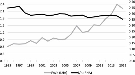
Additions to fixed assets/operating income (I/π) and financial assets/fixed assets (FA/K), full sample, 1995–2015.
Source: Authors’ elaboration based on Worldscope data.
Figure 2 shows that, on average, the rate of capital accumulation (I/K) of NFCs in DEEs experienced a decrease during 1995–1999, recovered in the run-up to the 2008 crisis, and decreased again after the crisis. At the same time, both financial payments (dividends plus interest as a ratio to fixed assets) and financial incomes have been increasing significantly. The 2007–2008 crisis has led to a slight reversal in the NFCs’ financial payments and incomes, although the increasing trends re-emerged thereafter.10
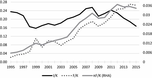
Rate of accumulation (I/K), financial payments/fixed assets (F/K) and financial incomes/fixed assets (πF/K), full sample, 1995–2015.
Source: Authors’ elaboration based on Worldscope data
Supplementary Table 4A provides the data description and sources for country-level variables. All these variables are constructed by calculating the average value from 1995 to 2007, to avoid taking into consideration the years of the financial crisis.11
The de facto index of financial development is the average of the stock market and financial intermediaries’ development in the country, including domestic credit to the private sector, stock market capitalisation, stock market total value traded and the stock market turnover ratio (all as a percent to GDP). This is a widely used index in the literature on the effect of financial development on growth or investment (e.g. see Love, 2003). The financial reform index (Abiad et al., 2010) is a de jure index normalised between 0 and 1 aiming at summarising indicators regarding legislation about controls on credit, interest rates, pro-competition measures, banking supervision, privatisation, international capital flows and the security markets.
The ratio of total financial liabilities to GDP is used as a proxy for the level of openness to foreign investors and captures the de facto capital account openness. Data are from the Lane and Milesi-Ferretti (2007) database. This measure includes all foreign liabilities in the form of portfolio and FDI investments. The widely used Chinn-Ito index (KaOpen) is employed to measure de jure capital account openness.
To capture the internationalisation of production we use the Global Value Chain (GVC) Participation Index provided by the UNCTAD-Eora GVC Database (UNCTAD, 2022). This index is better suited to capture the multi-faceted aspects of the integration of DEEs into GVCs compared to the simple offshoring measures (Milberg, 2008; Aslam et al., 2017). The index is equal to the sum of the share of foreign value-added in the country i’s exports and the share of country i’s value-added in foreign countries’ exports (indirect value-added), divided by the total value-added of exports.
Table 2 summarises the country-level variables.
Country-specific variables, average 1995–2008a
| Country | Financial development index | Financial reform index | Financial liabilities to GDP | Capital account openness index (Chinn-Ito) | Global Value Chain Participation Index |
|---|---|---|---|---|---|
| Argentina | −0.662 | 0.749 | 0.915 | 0.413 | 0.359 |
| Brazil | −0.242 | 0.515 | 0.546 | −0.768 | 0.405 |
| Chile | −0.040 | 0.835 | 0.975 | 0.485 | 0.488 |
| Colombia | 1.271 | 0.334 | 0.513 | −1.195 | 0.390 |
| China | −0.684 | 0.680 | 0.353 | −0.922 | 0.332 |
| Egypt, Arab Rep. | 0.082 | 0.675 | 0.623 | 1.574 | 0.443 |
| India | 0.120 | 0.506 | 0.346 | −1.195 | 0.399 |
| Indonesia | −0.330 | 0.606 | 0.879 | 1.326 | 0.463 |
| Korea, Rep. | 1.032 | 0.719 | 0.520 | −0.458 | 0.520 |
| Malaysia | 1.521 | 0.714 | 1.037 | 0.168 | 0.643 |
| Mexico | −0.645 | 0.866 | 0.574 | 0.919 | 0.420 |
| Nigeria | −0.842 | 0.729 | 0.981 | −0.999 | 0.408 |
| Pakistan | 0.376 | 0.511 | 0.504 | −1.249 | 0.316 |
| Peru | −0.645 | 0.896 | 0.723 | 2.233 | 0.453 |
| Philippines | −0.201 | 0.760 | 0.810 | 0.100 | 0.644 |
| Russian Federation | −0.564 | 0.744 | 0.692 | −0.544 | 0.574 |
| Singapore | 1.609 | 0.900 | 6.228 | 2.211 | 0.782 |
| South Africa | 0.955 | 0.847 | 0.676 | −1.113 | 0.531 |
| Sri Lanka | −0.582 | 0.629 | 0.663 | 0.100 | 0.380 |
| Thailand | 1.009 | 0.643 | 0.891 | −0.212 | 0.514 |
| Turkey | −0.096 | 0.703 | 0.552 | −1.113 | 0.505 |
| Median | −0.096 | 0.714 | 0.676 | −0.212 | 0.453 |
| Average | 0.116 | 0.693 | 0.952 | −0.011 | 0.475 |
| Min | −0.842 | 0.334 | 0.346 | −1.249 | 0.316 |
| Max | 1.609 | 0.900 | 6.228 | 2.233 | 0.782 |
Notes:
The light grey colour indicates that the respective country is above the median for a particular indicator. All the institutional variables used in our estimations are averaged for the period 1995–2007, to avoid considering turbulent years around the great financial crisis.
Sources: Authors’ elaboration based on World Bank, IMF, Chinn and Ito (2008), Lane and Milesi-Ferretti (2007) and UNCTAD. See Supplementary Table 4A for more information.
Although the rankings of the different indicators show some overlaps, the median splits based on different country-specific dimensions produce a rich and diverse categorisation.12 The various clusters constitute the sub-panels for the estimations.
4.1 Estimation methodology
In dynamic panel data models, the unobserved panel-level effects are correlated with the lagged dependent variables, and standard estimators (e.g. ordinary or generalised least squares) are inconsistent. Therefore, we estimate our model using a difference-Generalised Methods of Moments (GMM) estimator (Arellano and Bond, 1991). This methodology is suitable for analyses based on a ‘small-time/large observations’ sample. GMM is a powerful estimator for analyses based on firm-level data mainly for three reasons (Roodman, 2009). First, GMM is one of the best techniques to control for all sources of endogeneity between the dependent and explanatory variables, by using internal instruments, namely the lagged levels of the explanatory variables, which allows us to address dual causality if rising financial payments and incomes are also consequences of the slowdown in accumulation. The instrument set consists of instruments not correlated with the first difference of the error term but correlated with the dependent variable. Second, by first-differencing, this estimator eliminates companies’ unobservable fixed effects. Third, GMM can efficiently address auto-correlation problems. We apply two tests to assess the appropriateness of the instrument sets and lag structures. First, we check for second-order serial correlation with the Arellano-Bond test (Arellano and Bond, 1991). Second, we verify the validity of the instruments through the Hansen test.13 In all models, both the lagged dependent variable and all the explanatory variables enter the instrument set as endogenous regressors. Consistent with the structure of the GMM estimator, all the variables in the different specifications are instrumented using the second and third lags of the specific variables, while the year dummies are included in the exogenous set of instruments. We test the joint significance of the time dummies and the significance of the interaction dummies on financial income using a Wald test.
All the variables are in logarithmic form. We employ a log–log specification for five reasons: (i) to allow for non-linear relationships between the dependent and the explanatory variables; (ii) to control for heteroskedasticity; (iii) to allow for more meaningful interpretation of effects as elasticities (in percentage changes); (iv) to allow for direct comparison with previous micro-level studies about financialisation and in particular with Orhangazi (2008) and Tori and Onaran (2018, 2020); and (v) this form has proven to be more robust (in terms of auto-correlation and Hansen tests) when testing microeconomic relationship along with macroeconomic (institutional) variables (see e.g. Tori and Onaran, 2020). Robust standard errors are calculated through a two-step procedure, after a finite-sample correction (Windmeijer, 2005).
The country groupings are defined by computing the average of each indicator during the pre-crisis period 1995–2007, and by applying a median split between countries. All the estimations for the country groups come from weighted regressions, with the weights equal to 1 divided by the number of available observations in that country. This procedure mitigates the bias due to the high number of observations in some countries and allows considering country-specific time-invariant characteristics in a dynamic estimation (see Love, 2003).
5. Estimation results
This section presents the estimation results for alternative specifications of the investment model presented in Section 3. Table 3 presents the estimation results for the baseline model in equations (1) and (2) for the sample period of 1995–2015. The estimation results for specification (I) show both lagged accumulation and sales (i.e. demand) having a positive and highly significant effect on NFCs’ rate of accumulation. Also, operating profit has a positive effect on investment, although both its magnitude and significance level are relatively lower than the two previous variables. These results are in line with the evidence for NFCs in developed countries. In particular, the effect of profitability on capital accumulation is weak, and this could be directly due to the interaction between profits and the two financialisation channels described in Section 2.
Estimation results, full sample, dependent variable (I/K)t
| (I) | (II) | (III) | (IV) | (V) | (VI) | |
|---|---|---|---|---|---|---|
| TOT | TA10 | TA25 | TA50 | TA75 | TA90 | |
| 0.374*** | 0.372*** | 0.375*** | 0.378*** | 0.374*** | 0.369*** | |
| (0.025) | (0.025) | (0.024) | (0.024) | (0.026) | (0.025 | |
| 0.379*** | 0.375*** | 0.364*** | 0.344*** | 0.345*** | 0.365*** | |
| (0.051) | (0.053) | (0.053) | (0.054) | (0.051) | (0.049) | |
| 0.022* | 0.023* | 0.024* | 0.028** | 0.027** | 0.026** | |
| (0.013) | (0.013) | (0.013) | (0.013) | (0.013) | (0.013) | |
| −0.068** | −0.070** | −0.072*** | −0.084*** | −0.068*** | −0.071*** | |
| (0.028) | (0.028) | (0.028) | (0.027) | (0.026) | (0.025) | |
| −0.024 | −0.019 | 0.012 | 0.187*** | 0.346*** | 0.750** | |
| (0.022) | (0.024) | (0.035) | (0.058) | (0.120) | (0.352) | |
| −0.029 | −0.109 | −0.350*** | −0.455*** | −0.827** | ||
| (0.167) | (0.085) | (0.092) | (0.144) | (0.375) | ||
| −0.058*** | −0.058*** | −0.061*** | −0.062*** | −0.061*** | −0.057*** | |
| (0.017) | (0.016) | (0.017) | (0.015) | (0.014) | (0.017) | |
| Number of observations | 27885 | 27885 | 27885 | 27885 | 27885 | 27885 |
| Number of firms | 3720 | 3720 | 3720 | 3720 | 3720 | 3720 |
| Average number of observations | 7.5 | 7.5 | 7.5 | 7.5 | 7.5 | 7.5 |
| Number of instruments | 31 | 33 | 33 | 33 | 33 | 33 |
| p-value Hanses test | 0.199 | 0.265 | 0.301 | 0.233 | 0.206 | 0.323 |
| p-value A-B test (AR1) | 0.000 | 0.000 | 0.000 | 0.000 | 0.000 | 0.000 |
| p-value A-B test (AR2) | 0.423 | 0.419 | 0.479 | 0.813 | 0.772 | 0.803 |
| Time effects | Yes | Yes | Yes | Yes | Yes | Yes |
| p-value Wald test for time effects | 0.008 | 0.002 | 0.001 | 0.000 | 0.005 | 0.002 |
| p-value | 0.210 | 0.130 | 0.001 | 0.002 | 0.019 |
Notes: Weighted regressions (w=1/total country obs.), two-step difference-GMM estimations. Specification I is based on equation (1) and specifications II–VI based on equation (2). Coefficients for the year dummies are not reported. Robust corrected standard error in parenthesis.
Significant at 10%.
Significant at 5%.
Significant at 1.
Source: authors’ computations based on Worldscope data.
The average effect of financial payments (interest plus dividends) is negative and significant, while financial income is insignificant. Also, the ratio of debt to total assets has a significantly negative effect on capital accumulation, indicating that debt has constrained investment in the DEEs.
Columns II–IV of Table 3 shows the estimation results for equation (2), in which the effect of financial income interacts with the firm sizes measured by total assets. In specification II, the dummy variable is equal to 1 for companies in the bottom 10% in terms of size distribution, while in specification VI, = 1 for companies in the bottom 90% in terms of size distribution. The other thresholds in terms of size are the first, second and third quartiles (i.e. 25, 50 and 75%). An interesting finding is that larger NFCs from the top 50% to the top 10% experienced a positive effect of financial income on investment (columns IV–VI). The elasticity for financial income across these percentiles is equal to +0.43 on average for the relatively larger companies, while for the smaller firms, this is between −0.16 and −0.77.14 This result stands in stark contrast to the ones so far proposed by the literature on developed economies (e.g. see Orhangazi, 2008; Tori and Onaran, 2018, 2020), where cash-constrained smaller companies experience generally positive effects of financial incomes on their investment. This result can be explained from a ‘catching-up’ perspective, where larger companies in DEEs aim at improving their productive basis to compete with competitors operating in developed countries, also utilising income from financial investments, whereas smaller companies seem to favour (reversible) financial investment over (irreversible) fixed capital expenditures.15 The effects of both financial payments and debt on investment are consistently negative and significant in all estimations.
Next, we present the results of the tests of the three hypotheses presented in Section 2 regarding the effect of country-specific features on the effects of financialisation at the firm level. The sub-panel including NFCs in countries with indicators below the median is named ‘panel 0’, while ‘panel 1’ is used to indicate NFCs in countries above the median.
The first set of estimations tests the variation in the effects of financialisation on NFCs with respect to the financial development and reform of the country, testing hypothesis 1. Tables 4 and 7 present the estimation results from the median split based on the composite index of financial development and the financial reform index, respectively.
Estimation results, full sample, 1995–2015, financial development index median split, dependent variable (I/K)t
| Financial development index below the median | Financial development index above the median | |||||||||||
|---|---|---|---|---|---|---|---|---|---|---|---|---|
| (I) | (II) | (III) | (IV) | (V) | (VI) | (VII) | (VIII) | (IX) | (X) | (XI) | (XII) | |
| TOT | TA10 | TA25 | TA50 | TA75 | TA90 | TOT | TA10 | TA25 | TA50 | TA75 | TA90 | |
| 0.295*** | 0.283*** | 0.294*** | 0.310*** | 0.307*** | 0.301*** | 0.440*** | 0.432*** | 0.437*** | 0.443*** | 0.430*** | 0.420*** | |
| (0.042) | (0.041) | (0.039) | (0.040) | (0.042) | (0.041) | (0.028) | (0.029) | (0.029) | (0.029) | (0.034) | (0.040) | |
| 0.282*** | 0.291*** | 0.244*** | 0.229** | 0.281*** | 0.268*** | 0.411*** | 0.421*** | 0.427*** | 0.404*** | 0.378*** | 0.396*** | |
| (0.084) | (0.085) | (0.089) | (0.091) | (0.082) | (0.080) | (0.053) | (0.053) | (0.055) | (0.056) | (0.058) | (0.065) | |
| 0.021 | 0.024 | 0.025 | 0.026 | 0.020 | 0.023 | 0.021 | 0.018 | 0.021 | 0.020 | 0.023 | 0.029 | |
| (0.022) | (0.022) | (0.021) | (0.021) | (0.021) | (0.022) | (0.016) | (0.016) | (0.016) | (0.016) | (0.015) | (0.019) | |
| −0.069 | −0.078 | −0.078 | −0.094** | −0.067 | −0.069* | −0.067*** | −0.061** | −0.069*** | −0.068*** | −0.068*** | −0.073** | |
| (0.047) | (0.049) | (0.049) | (0.048) | (0.044) | (0.042) | (0.025) | (0.027) | (0.026) | (0.025) | (0.026) | (0.032) | |
| −0.034 | −0.023 | 0.034 | 0.219** | 0.350** | 0.645** | −0.005 | −0.024 | −0.026 | 0.085 | 0.328*** | 1.262 | |
| (0.035) | (0.042) | (0.052) | (0.086) | (0.160) | (0.277) | (0.022) | (0.030) | (0.049) | (0.059) | (0.124) | (0.907) | |
| −0.022 | −0.184* | −0.398*** | −0.467** | −0.724** | 0.765 | 0.108 | −0.188 | −0.437*** | −1.373 | |||
| (0.089) | (0.105) | (0.124) | (0.190) | (0.295) | (0.740) | (0.224) | (0.122) | (0.161) | (0.975) | |||
| −0.027 | −0.030 | −0.032 | −0.035 | −0.043* | −0.028 | −0.070*** | −0.067*** | −0.068*** | −0.074*** | −0.065*** | −0.066*** | |
| (0.029) | (0.029) | (0.030) | (0.027) | (0.026) | (0.030) | (0.014) | (0.014) | (0.014) | (0.014) | (0.013) | (0.014) | |
| Number of observations | 6,436 | 6,436 | 6,436 | 6,436 | 6,436 | 6,436 | 21,449 | 21,449 | 21,449 | 21,449 | 21,449 | 21,449 |
| Number of firms | 767 | 767 | 767 | 767 | 767 | 767 | 2,953 | 2,953 | 2,953 | 2,953 | 2,953 | 2,953 |
| Average number of observations | 8.4 | 8.4 | 8.4 | 8.4 | 8.4 | 8.4 | 7.3 | 7.3 | 7.3 | 7.3 | 7.3 | 7.3 |
| Number of instruments | 31 | 33 | 33 | 33 | 33 | 33 | 31 | 33 | 33 | 33 | 33 | 33 |
| p-value Hanses test | 0.514 | 0.531 | 0.618 | 0.476 | 0.545 | 0.638 | 0.044 | 0.123 | 0.036 | 0.019 | 0.112 | 0.222 |
| p-value A-B test (AR1) | 0.000 | 0.000 | 0.000 | 0.000 | 0.000 | 0.000 | 0.000 | 0.000 | 0.000 | 0.000 | 0.000 | 0.000 |
| p-value A-B test (AR2) | 0.838 | 0.837 | 0.918 | 0.729 | 0.744 | 0.855 | 0.426 | 0.682 | 0.502 | 0.421 | 0.485 | 0.918 |
| Time effects | Yes | Yes | Yes | Yes | Yes | Yes | Yes | Yes | Yes | Yes | Yes | Yes |
| Wald test for time effects (p-value) | 0.002 | 0.001 | 0.000 | 0.005 | 0.001 | 0.000 | 0.010 | 0.008 | 0.009 | 0.012 | 0.004 | 0.003 |
| p-value | 0.514 | 0.058 | 0.005 | 0.022 | 0.057 | 0.304 | 0.650 | 0.026 | 0.144 | |||
Notes: Weighted regressions (w=1/total country obs.), two-step difference-GMM estimations. Specifications I and VII are based on equation (1) and specifications II–VI and VIII–XII based on equation (2). Coefficients for the year dummies are not reported. Robust corrected standard error in parenthesis.
Significant at 10%.
Significant at 5%.
Significant at 1%.
Source: Authors’ computations based on Worldscope data.
Estimation results, full sample, 1995–2015, financial reform index median split, dependent variable (I/K)t
| Financial reform index below the median | Financial reform index above the median | |||||||||||
|---|---|---|---|---|---|---|---|---|---|---|---|---|
| (I) | (II) | (III) | (IV) | (V) | (VI) | (VII) | (VIII) | (IX) | (X) | (XI) | (XII) | |
| TOT | TA10 | TA25 | TA50 | TA75 | TA90 | TOT | TA10 | TA25 | TA50 | TA75 | TA90 | |
| 0.408*** | 0.412*** | 0.404*** | 0.397*** | 0.397*** | 0.399*** | 0.324*** | 0.326*** | 0.325*** | 0.344*** | 0.345*** | 0.328*** | |
| (0.032) | (0.032) | (0.032) | (0.034) | (0.035) | (0.033) | (0.036) | (0.035) | (0.035) | (0.036) | (0.040) | (0.039) | |
| 0.457*** | 0.463*** | 0.415*** | 0.405*** | 0.413*** | 0.440*** | 0.345*** | 0.345*** | 0.364*** | 0.333*** | 0.345*** | 0.325*** | |
| (0.068) | (0.081) | (0.076) | (0.077) | (0.073) | (0.068) | (0.069) | (0.069) | (0.068) | (0.067) | (0.069) | (0.069) | |
| −0.008 | −0.008 | 0.004 | 0.005 | 0.006 | −0.005 | 0.057*** | 0.058*** | 0.058*** | 0.054*** | 0. 051*** | 0.054*** | |
| (0.020) | (0.022) | (0.019) | (0.020) | (0.020) | (0.020) | (0.014) | (0.014) | (0.014) | (0.015) | (0.015) | (0.015) | |
| −0.018 | −0.025 | −0.017 | −0.014 | −0.018 | −0.024 | −0.129*** | −0.128*** | −0.129*** | −0.159*** | −0.120*** | −0.111*** | |
| (0.034) | (0.034) | (0.033) | (0.032) | (0.033) | (0.033) | (0.036) | (0.036) | (0.036) | (0.038) | (0.037) | (0.038) | |
| −0.018 | −0.026 | 0.065 | 0.160** | 0.224** | 0.316* | −0.062** | −0.067* | −0.067* | 0.192 | 0.238 | 0.392 | |
| (0.027) | (0.037) | (0.059) | (0.075) | (0.103) | (0.184) | (0.028) | (0.036) | (0.038) | (0.191) | (0.237) | (0.585) | |
| 0.316 | −0.344 | −0.374** | −0.317** | −0.361* | 0.013 | 0.026 | −0.365*** | −0.351 | −0.478 | |||
| (0.506) | (0.231) | (0.154) | (0.130) | (0.193) | (0.074) | (0.085) | (0.129) | (0.272) | (0.625) | |||
| −0.109*** | −0.106*** | −0.130*** | −0.126*** | −0.115*** | −0.106*** | −0.027 | −0.028 | −0.029 | −0.028 | −0.026 | −0.027 | |
| (0.018) | (0.018) | (0.024) | (0.022) | (0.019) | (0.019) | (0.024) | (0.024) | (0.024) | (0.019) | (0.016) | (0.025) | |
| Number of observations | 15,029 | 15,029 | 15,029 | 15,029 | 15,029 | 15,029 | 12,856 | 12,856 | 12,856 | 12,856 | 12,856 | 12,856 |
| Number of firms | 2,054 | 2,054 | 2,054 | 2,054 | 2,054 | 2,054 | 1,666 | 1,666 | 1,666 | 1,666 | 1,666 | 1,666 |
| Average number of observations | 7.3 | 7.3 | 7.3 | 7.3 | 7.3 | 7.3 | 7.7 | 7.7 | 7.7 | 7.7 | 7.7 | 7.7 |
| Number of instruments | 31 | 33 | 33 | 33 | 33 | 33 | 31 | 33 | 33 | 33 | 33 | 33 |
| p-value Hanses test | 0.324 | 0.426 | 0.569 | 0.268 | 0.138 | 0.198 | 0.199 | 0.276 | 0.233 | 0.182 | 0.308 | 0.140 |
| p-value A-B test (AR1) | 0.000 | 0.000 | 0.000 | 0.000 | 0.000 | 0.000 | 0.000 | 0.000 | 0.000 | 0.000 | 0.000 | 0.000 |
| p-value A-B test (AR2) | 0.744 | 0.807 | 0.663 | 0.995 | 0.870 | 0.821 | 0.591 | 0.601 | 0.530 | 0.840 | 0.735 | 0.755 |
| Time effects | Yes | Yes | Yes | Yes | Yes | Yes | Yes | Yes | Yes | Yes | Yes | Yes |
| Wald test for time effects (p-value) | 0.002 | 0.000 | 0.009 | 0.000 | 0.003 | 0.002 | 0.001 | 0.000 | 0.005 | 0.006 | 0.002 | 0.000 |
| p-value | 0.550 | 0.130 | 0.020 | 0.028 | 0.124 | 0.312 | 0.517 | 0.000 | 0.025 | 0.093 | ||
Notes: Weighted regressions (w=1/total country obs.), two-step difference-GMM estimations. Specifications I and VII are based on equation (1) and specifications II–VI and VIII–XII based on equation (2). Coefficients for the year dummies are not reported. Robust corrected standard error in parenthesis.
Significant at 10%.
Significant at 5%.
Significant at 1%.
Source: Authors’ computations based on Worldscope data.
The results in Table 4 show that the split in terms of financial development is inconclusive, in particular given the low Hansen’s test for estimation in panel 1. A lower level of financial development is associated with a positive effect of financial incomes on investment for larger companies and a negative effect for smaller ones (see columns IV, V and VI). The inability of the financial development index in explaining countries’ differences might be due to diverging effects from its two sub-components. Financial development is, in fact, the combination of two indices: INDEX1 summarises the development of financial intermediaries, while INDEX2 measures the development and efficiency of the stock market. Thus, we provide disaggregated estimations for these two indices in Tables 5 and 6. The estimations based on the split based on INDEX1 still suffer from the poor instrument sets. On the contrary, estimations based on INDEX2 provide useful insights. Results in column VII of Table 6 show that the aggregate effect of both financial payments and incomes is significant and negative for NFCs in countries with a relatively higher development of their stock markets. In countries with lower levels of stock market development, the investments of larger NFCs in the top 50% benefited from financial incomes (0.23), while the effect has been slightly negative for the rest of the companies (−0.015).
Estimation results, full sample, 1995–2015, INDEX1 index median split, dependent variable (I/K)t
| INDEX1 below the median | INDEX1 above the median | |||||||||||
|---|---|---|---|---|---|---|---|---|---|---|---|---|
| (I) | (II) | (III) | (IV) | (V) | (VI) | (VII) | (VIII) | (IX) | (X) | (XI) | (XII) | |
| TOT | TA10 | TA25 | TA50 | TA75 | TA90 | TOT | TA10 | TA25 | TA50 | TA75 | TA90 | |
| 0.332*** | 0.324*** | 0.330*** | 0. 336*** | 0.346*** | 0.329*** | 0.403*** | 0.402*** | 0.401*** | 0.404*** | 0.399*** | 0.400*** | |
| (0.043) | (0.044) | (0.042) | (0.043) | (0.048) | (0.043) | (0.024) | (0.024) | (0.024) | (0.024) | (0.025) | (0.026) | |
| 0.350*** | 0.349*** | 0.281*** | 0.298*** | 0.319*** | 0.353*** | 0.402*** | 0.404*** | 0.410*** | 0.382*** | 0.384*** | 0.367*** | |
| (0.092) | (0.094) | (0.102) | (0.103) | (0.096) | (0.088) | (0.048) | (0.048) | (0.049) | (0.050) | (0.050) | (0.057) | |
| 0.013 | 0.016 | 0.023 | 0.022 | 0.028 | 0.025 | 0.027** | 0.026* | 0.026* | 0.024* | 0.027* | 0.028** | |
| (0.023) | (0.023) | (0.023) | (0.023) | (0.025) | (0.023) | (0.013) | (0.013) | (0.013) | (0.014) | (0.014) | (0.014) | |
| −0.053 | −0.058 | −0.066 | −0.085* | −0.067 | −0.073 | −0.096*** | −0.094*** | −0.099*** | −0.096*** | −0.092*** | −0.081*** | |
| (0.045) | (0.047) | (0.049) | (0.048) | (0.045) | (0.045) | (0.022) | (0.022) | (0.022) | (0.023) | (0.023) | (0.025) | |
| −0.035 | −0.020 | 0.060 | 0.228** | 0.531** | 0.853* | 0.002 | −0.003 | −0.010 | 0.097* | 0.172* | 0.801 | |
| (0.036) | (0.042) | (0.059) | (0.100) | (0.252) | (0.496) | (0.020) | (0.023) | (0.031) | (0.049) | (0.096) | (0.607) | |
| −0.053 | −0.254* | −0.413*** | −0.689** | −0.950* | 0.173 | 0.063 | −0.191* | −0.222* | −0.866 | |||
| (0.098) | (0.133) | (0.148) | (0.295) | (0.527) | (0.272) | (0.102) | (0.102) | (0.125) | (0.653) | |||
| −0.052* | −0.055* | −0.059** | −0.060** | −0.066*** | −0.046 | −0.055*** | −0.055*** | −0.053*** | −0.055*** | −0.053*** | −0.057*** | |
| (0.029) | (0.028) | (0.029) | (0.026) | (0.023) | (0.029) | (0.014) | (0.014) | (0.014) | (0.014) | (0.014) | (0.014) | |
| Number of observations | 5612 | 5612 | 5612 | 5612 | 5612 | 5612 | 22273 | 22273 | 22273 | 22273 | 22273 | 22273 |
| Number of firms | 664 | 664 | 664 | 664 | 664 | 664 | 3056 | 3056 | 3056 | 3056 | 3056 | 3056 |
| Average number of observations | 8.5 | 8.5 | 8.5 | 8.5 | 8.5 | 8.5 | 7.3 | 7.3 | 7.3 | 7.3 | 7.3 | 7.3 |
| Number of instruments | 31 | 33 | 33 | 33 | 33 | 33 | 31 | 33 | 33 | 33 | 33 | 33 |
| p−value Hanses test | 0.608 | 0.652 | 0.739 | 0.668 | 0.776 | 0.760 | 0.012 | 0.023 | 0.009 | 0.002 | 0.006 | 0.073 |
| p-value A-B test (AR1) | 0.000 | 0.000 | 0.000 | 0.000 | 0.000 | 0.000 | 0.000 | 0.000 | 0.000 | 0.000 | 0.000 | 0.000 |
| p-value A-B test (AR2) | 0.337 | 0.323 | 0.632 | 0.802 | 0.674 | 0.488 | 0.715 | 0.641 | 0.647 | 0.678 | 0.564 | 0.243 |
| Time effects | yes | yes | yes | yes | yes | yes | yes | yes | yes | yes | yes | Yes |
| Wald test for time effects (p-value) | 0.002 | 0.003 | 0.002 | 0.000 | 0.001 | 0.002 | 0.017 | 0.009 | 0.031 | 0.036 | 0.044 | 0.012 |
| p-value | 0.351 | 0.051 | 0.012 | 0.012 | 0.056 | 0.518 | 0.520 | 0.123 | 0.195 | 0.221 | ||
Notes: Weighted regressions (w=1/total country obs.), two-step difference-GMM estimations. Specifications I and VII are based on equation (1) and specifications II–VI and VIII–XII based on equation (2). Coefficients for the year dummies are not reported. Robust corrected standard error in parenthesis.
Significant at 10%.
Significant ant 5%.
Significant at 1%.
Source: Authors’ computations based on Worldscope data.
Estimation results, full sample, 1995–2015, INDEX2 index median split, dependent variable (I/K)t
| INDEX2 below the median | INDEX2 above the median | |||||||||||
|---|---|---|---|---|---|---|---|---|---|---|---|---|
| (I) | (II) | (III) | (IV) | (V) | (VI) | (VII) | (VIII) | (IX) | (X) | (XI) | (XII) | |
| TOT | TA10 | TA25 | TA50 | TA75 | TA90 | TOT | TA10 | TA25 | TA50 | TA75 | TA90 | |
| 0.336*** | 0.327*** | 0.334*** | 0.356*** | 0.350*** | 0.342*** | 0.424*** | 0.423*** | 0.437*** | 0.421*** | 0.387*** | 0.393*** | |
| (0.043) | (0.042) | (0.042) | (0.041) | (0.044) | (0.043) | (0.026) | (0.026) | (0.026) | (0.027) | (0.035) | (0.043) | |
| 0.439*** | 0.443*** | 0.413*** | 0.386*** | 0.419*** | 0.416*** | 0.330*** | 0.338*** | 0.357*** | 0.346*** | 0.305*** | 0.312*** | |
| (0.085) | (0.086) | (0.090) | (0.092) | (0.086) | v0.083) | (0.050) | (0.049) | (0.050) | (0.050) | (0.052) | (0.054) | |
| −0.003 | −0.000 | 0.001 | 0.007 | 0.001 | −0.001 | 0.042*** | 0.040** | 0.041*** | 0.038** | 0.037*** | 0.049*** | |
| (0.021) | (0.021) | (0.021) | (0.021) | (0.021) | (0.021) | (0.015) | (0.016) | (0.015) | (0.015) | (0.014) | (0.017) | |
| −0.072 | −0.077* | −0.078* | −0.088** | −0.064 | −0.066 | −0.065** | −0.063** | −0.070*** | −0.065** | −0.070*** | −0.070** | |
| (0.045) | (0.046) | (0.046) | (0.044) | (0.042) | (0.041) | (0.027) | (0.027) | (0.027) | (0.027) | (0.026) | (0.032) | |
| −0.001 | 0.005 | 0.044 | 0.234*** | 0.250** | 0.396* | −0.039* | −0.048* | −0.035 | 0.060 | 0.405** | 1.283 | |
| (0.032) | (0.038) | (0.048) | (0.077) | (0.123) | (0.228) | (0.021) | (0.025) | (0.028) | (0.059) | (0.158) | (1.081) | |
| −0.022 | −0.131 | −0.379*** | −0.303** | −0.425* | 0.295 | 0.006 | −0.202* | −0.577*** | −1.420 | |||
| (0.107) | (0.111) | (0.120) | (0.151) | (0.247) | (0.391) | (0.091) | (0.111) | (0.198) | (1.162) | |||
| −0.040 | −0.043 | −0.044 | −0.049* | −0.049* | −0.040 | −0.068*** | −0.068*** | −0.071*** | −0.074*** | −0.060*** | −0.062*** | |
| (0.028) | (0.027) | (0.028) | (0.026) | (0.026) | (0.028) | (0.014) | (0.014) | (0.013) | (0.013) | (0.013) | (0.014) | |
| Number of observations | 4782 | 4782 | 4782 | 4782 | 4782 | 4782 | 23103 | 23103 | 23103 | 23103 | 23103 | 23103 |
| Number of firms | 621 | 621 | 621 | 621 | 621 | 621 | 3099 | 3099 | 3099 | 3099 | 3099 | 3099 |
| Average number of observations | 7.7 | 7.7 | 7.7 | 7.7 | 7.7 | 7.7 | 7.5 | 7.5 | 7.5 | 7.5 | 7.5 | 7.5 |
| Number of instruments | 31 | 33 | 33 | 33 | 33 | 33 | 31 | 33 | 33 | 33 | 33 | 33 |
| p-value Hanses test | 0.409 | 0.462 | 0.503 | 0.412 | 0.344 | 0.493 | 0.229 | 0.208 | 0.051 | 0.026 | 0.060 | 0.199 |
| p-value A-B test (AR1) | 0.000 | 0.000 | 0.000 | 0.000 | 0.000 | 0.000 | 0.000 | 0.000 | 0.000 | 0.000 | 0.000 | 0.000 |
| p-value A-B test (AR2) | 0.650 | 0.634 | 0.562 | 0.335 | 0.445 | 0.448 | 0.208 | 0.223 | 0.095 | 0.121 | 0.141 | 0.225 |
| Time effects | Yes | Yes | Yes | Yes | Yes | Yes | Yes | Yes | Yes | Yes | Yes | Yes |
| Wald test for time effects (p-value) | 0.001 | 0.002 | 0.002 | 0.000 | 0.004 | 0.002 | 0.002 | 0.001 | 0.012 | 0.026 | 0.014 | 0.002 |
| p-value | 0.852 | 0.300 | 0.024 | 0.256 | 0.462 | 0.512 | 0.692 | 0.021 | 0.001 | 0.110 | ||
Notes: Weighted regressions (w=1/total country obs.), two-step difference-GMM estimations. Specifications I and VII based on equation (1) and specifications II–VI and VIII–XII based on equation (2). Coefficients for the year dummies are not reported. Robust corrected standard error in parenthesis.
Significant at 10%.
Significant ant 5%.
Significant at 1%.
Source: Authors’ computations based on Worldscope data.
The clustering of companies based on the median levels of the financial reform index provides a clearer picture. Table 7 shows that, in aggregate, higher levels of the financial reform index are associated with the negative effects of both financial payments and incomes on investment (column VII). In particular, the effect of financial incomes is negative albeit insignificant for companies in the top percentiles. Legislations that favoured the liberalisations of financial markets seem to be associated with stronger negative effects of financial incomes for all NFCs. NFCs in countries where financial liberalisation reforms have been relatively modest in this period (e.g. Colombia, India and Pakistan) experience a positive effect of financial incomes for larger companies (from 0.16 to 0.22) and a negative effect for the ones below the second and third quartiles (columns IV and V). The ratio of total debt to total assets has a negative and significant effect only for NFCs in panel 0.
Taken together, the results for the financial development and reform indices provide support for hypothesis 2. Higher levels of stock market development and liberalisation of the financial sector in DEEs are associated with clearer negative effects of financialisation on NFCs’ investment.
The second institutional dimension within which the financialisation of the NFCs in DEEs is analysed relates to the variation with respect to the degrees of openness to foreign investment, testing hypothesis 2. The results in Table 8 show that there has been an aggregate negative effect of both financial payments and incomes in NFCs operating in countries with a relatively higher value of financial liabilities as a ratio to GDP (columns VII, VIII and IX). A slightly positive effect (0.14) of financial incomes is detected for companies in the top 50% of the distribution (column X). In countries where financial liabilities/GDP is relatively lower, the effect of financial payments is insignificant. Financial incomes have a positive effect on the investment of companies above the second and third quartiles of the size distribution and a negative effect for smaller companies (columns IV and V). NFCs in panel 0 experience an overall negative and highly significant effect of debt on investment. Interestingly, the results for the split based on financial liabilities resemble those for the split based on the financial reform index (see Table 7).
Estimation results, full sample, 1995–2015, total financial liabilities to GDP median split, dependent variable (I/K)t
| Financial liabilities to GDP above the median | Financial liabilities to GDP above the median | |||||||||||
|---|---|---|---|---|---|---|---|---|---|---|---|---|
| (I) | (II) | (III) | (IV) | (V) | (VI) | (VII) | (VIII) | (IX) | (X) | (XI) | (XII) | |
| TOT | TA10 | TA25 | TA50 | TA75 | TA90 | TOT | TA10 | TA25 | TA50 | TA75 | TA90 | |
| 0.397*** | 0.400*** | 0.389*** | 0.386*** | 0.393*** | 0.393*** | 0.346*** | 0.350*** | 0.347*** | 0.360*** | 0.354*** | 0.348*** | |
| (0.032) | (0.033) | (0.031) | (0.034) | (0.036) | (0.033) | (0.036) | (0.036) | (0.036) | (0.035) | (0.037) | (0.038) | |
| 0.415*** | 0.429*** | 0.365*** | 0.356*** | 0.372*** | 0.406*** | 0.362*** | 0.365*** | 0.388*** | 0.355*** | 0.358*** | 0.346*** | |
| (0.066) | (0.083) | (0.074) | (0.076) | (0.072) | (0.067) | (0.072) | (0.072) | (0.071) | (0.070) | (0.071) | (0.071) | |
| 0.003 | 0.002 | 0.014 | 0.016 | 0.018 | 0.005 | 0.049*** | 0.050*** | 0.050*** | 0.047*** | 0.044*** | 0.047*** | |
| (0.019) | (0.023) | (0.017) | (0.018) | (0.019) | (0.018) | (0.016) | (0.016) | (0.016) | (0.017) | (0.016) | (0.017) | |
| −0.040 | −0.051 | −0.040 | −0.038 | −0.038 | −0.044 | −0.100*** | −0.099*** | −0.101*** | −0.124*** | −0.091** | −0.081** | |
| (0.036) | (0.037) | (0.035) | (0.032) | (0.034) | (0.035) | (0.037) | (0.037) | (0.037) | (0.038) | (0.036) | (0.038) | |
| 0.004 | −0.010 | 0.107* | 0.216** | 0.272** | 0.288 | −0.073** | −0.084** | −0.078** | 0.139* | 0.179 | 0.458 | |
| (0.025) | (0.045) | (0.065) | (0.085) | (0.121) | (0.197) | (0.029) | (0.037) | (0.037) | (0.077) | (0.159) | (0.585) | |
| 0.412 | −0.405 | −0.420** | −0.348** | −0.309 | 0.038 | 0.030 | −0.305*** | −0.295 | −0.566 | |||
| (0.776) | (0.255) | (0.164) | (0.153) | (0.209) | (0.079) | (0.080) | (0.112) | (0.184) | (0.621) | |||
| −0.084*** | −0.082*** | −0.106*** | −0.099*** | −0.091*** | −0.080*** | −0.042 | −0.043 | −0.043 | −0.044** | −0.042** | −0.041 | |
| (0.017) | (0.017) | (0.022) | (0.020) | (0.018) | (0.017) | (0.027) | (0.027) | (0.027) | (0.022) | (0.019) | (0.028) | |
| Number of observations | 18,860 | 18,860 | 18,860 | 18,860 | 18,860 | 18,860 | 9,025 | 9,025 | 9,025 | 9,025 | 9,025 | 9,025 |
| Number of firms | 2,668 | 2,668 | 2,668 | 2,668 | 2,668 | 2,668 | 1,052 | 1,052 | 1,052 | 1,052 | 1,052 | 1,052 |
| Average number of observations | 7.1 | 7.1 | 7.1 | 7.1 | 7.1 | 7.1 | 8.6 | 8.6 | 8.6 | 8.6 | 8.6 | 8.6 |
| Number of instruments | 31 | 33 | 33 | 33 | 33 | 33 | 31 | 33 | 33 | 33 | 33 | 33 |
| p-value Hanses test | 0.408 | 0.507 | 0.715 | 0.547 | 0.212 | 0.259 | 0.239 | 0.318 | 0.246 | 0.203 | 0.349 | 0.266 |
| p-value A-B test (AR1) | 0.000 | 0.000 | 0.000 | 0.000 | 0.000 | 0.000 | 0.000 | 0.000 | 0.000 | 0.000 | 0.000 | 0.000 |
| p-value A-B test (AR2) | 0.495 | 0.579 | 0.412 | 0.751 | 0.582 | 0.535 | 0.929 | 0.961 | 0.853 | 0.892 | 0.909 | 0.862 |
| Time effects | Yes | Yes | Yes | Yes | Yes | Yes | Yes | Yes | Yes | Yes | Yes | Yes |
| Wald test for time effects (p-value) | 0.000 | 0.002 | 0.001 | 0.000 | 0.003 | 0.002 | 0.002 | 0.001 | 0.002 | 0.004 | 0.005 | 0.001 |
| p-value | 0.588 | 0.135 | 0.024 | 0.012 | 0.487 | 0.445 | 0.430 | 0.002 | 0.123 | 0.033 | ||
Notes: Weighted regressions (w=1/total country obs.), two-step difference-GMM estimations. Specifications I and VII are based on equation (1) and specifications II–VI and VIII–XII based on equation (2). Coefficients for the year dummies are not reported. Robust corrected standard error in parenthesis.
Significant at 10%.
Significant at 5%.
Significant at 1%.
Source: Authors’ computations based on Worldscope data.
The estimations based on capital account openness confirm these findings. Using a de jure indicator of capital account openness, the aggregate effects of financial payments and incomes are negative and significant in panel 1 (Table 9, column VII). Both larger NFCs operating in countries with less and more open capital accounts experience a positive effect of financial incomes on investment. However, with lower capital account openness, this positive effect is particularly strong for NFCs in the top 10% of the size distribution (column VI), while it is slightly negative for the ones in the bottom 50% (−0.12, column IV); for higher levels of capital account openness the positive effect is particularly strong for NFCs in the top 25% of the size distribution, while it is significantly negative for the ones in the bottom 75% (−0.20, column XI). Also, the effect of financial payments is insignificant when the capital account is relatively less open, while a higher level of openness is also associated with a higher significance of the negative effect of debt. These results support our third hypothesis that countries with a higher degree of capital account openness (e.g. Argentina, Chile, Indonesia and Thailand) experience a stronger negative effect of financial incomes on NFCs’ investment.
Estimation results, full sample, 1995–2015, capital account openness index median split, dependent variable (I/K)t
| Capital account openness below the median | Capital account openness above the median | |||||||||||
|---|---|---|---|---|---|---|---|---|---|---|---|---|
| (I) | (II) | (III) | (IV) | (V) | (VI) | (VII) | (VIII) | (IX) | (X) | (XI) | (I) | |
| TOT | TA10 | TA25 | TA50 | TA75 | TA90 | TOT | TA10 | TA25 | TA50 | TA75 | TOT | |
| 0.365*** | 0.354*** | 0.359*** | 0.367*** | 0.367*** | 0.364*** | 0.400*** | 0.399*** | 0.413*** | 0.397*** | 0.384*** | 0.397*** | |
| (0.038) | (0.037) | (0.037) | (0.034) | (0.037) | (0.037) | (0.033) | (0.033) | (0.034) | (0.038) | (0.040) | (0.035) | |
| 0.464*** | 0.469*** | 0.457*** | 0.406*** | 0.444*** | 0.431*** | 0.330*** | 0.341*** | 0.343*** | 0.346*** | 0.294*** | 0.337*** | |
| (0.068) | (0.068) | (0.073) | (0.073) | (0.069) | (0.067) | (0.067) | (0.066) | (0.068) | (0.074) | (0.069) | (0.066) | |
| −0.001 | 0.004 | 0.000 | 0.008 | 0.001 | 0.001 | 0.041** | 0.040** | 0.042** | 0.041** | 0.041** | 0.046*** | |
| (0.019) | (0.019) | (0.019) | (0.019) | (0.019) | (0.019) | (0.017) | (0.017) | (0.017) | (0.018) | (0.017) | (0.017) | |
| −0.058 | −0.068 | −0.062 | −0.061 | −0.053 | −0.059 | −0.062* | −0.056 | −0.077** | −0.090*** | −0.066* | −0.071** | |
| (0.043) | (0.043) | (0.043) | (0.043) | (0.040) | (0.037) | (0.035) | (0.035) | (0.035) | (0.035) | (0.037) | (0.036) | |
| −0.013 | −0.007 | −0.003 | 0.175** | 0.178 | 0.615* | −0.056** | −0.080*** | −0.032 | 0.161* | 0. 424*** | 0.640 | |
| (0.030) | (0.035) | (0.048) | (0.077) | (0.130) | (0.320) | (0.026) | (0.031) | (0.036) | (0.090) | (0.163) | (0.552) | |
| −0.023 | −0.028 | −0.293*** | −0.228 | −0.658** | 0.453 | −0.082 | −0.441** | −0.622*** | −0.764 | |||
| (0.117) | (0.100) | (0.108) | (0.151) | (0.335) | (0.295) | (0.172) | (0.187) | (0.210) | (0.605) | |||
| −0.048* | −0.054* | −0.051* | −0.060** | −0.055** | −0.048* | −0.068*** | −0.067*** | −0.072*** | −0.073*** | −0.063*** | −0.066*** | |
| (0.029) | (0.028) | (0.028) | (0.026) | (0.025) | (0.029) | (0.019) | (0.019) | (0.019) | (0.017) | (0.017) | (0.018) | |
| Number of observations | 17,912 | 17,912 | 17,912 | 17,912 | 17,912 | 17,912 | 9,973 | 9,973 | 9,973 | 9,973 | 9,973 | 9,973 |
| Number of firms | 2,576 | 2,576 | 2,576 | 2,576 | 2,576 | 2,576 | 1,144 | 1,144 | 1,144 | 1,144 | 1,144 | 1,144 |
| Average number of observations | 7.0 | 7.0 | 7.0 | 7.0 | 7.0 | 7.0 | 8.7 | 8.7 | 8.7 | 8.7 | 8.7 | 8.7 |
| Number of instruments | 31 | 33 | 33 | 33 | 33 | 33 | 31 | 33 | 33 | 33 | 33 | 33 |
| p-value Hanses test | 0.139 | 0.138 | 0.182 | 0.174 | 0.160 | 0.191 | 0.444 | 0.698 | 0.296 | 0.211 | 0.273 | 0.604 |
| p-value A-B test (AR1) | 0.000 | 0.000 | 0.000 | 0.000 | 0.000 | 0.000 | 0.000 | 0.000 | 0.000 | 0.000 | 0.000 | 0.000 |
| p-value A-B test (AR2) | 0.459 | 0.421 | 0.422 | 0.249 | 0.262 | 0.208 | 0.141 | 0.168 | 0.121 | 0.242 | 0.162 | 0.175 |
| Time effects | Yes | Yes | Yes | Yes | Yes | Yes | Yes | Yes | Yes | Yes | Yes | Yes |
| Wald test for time effects (p-value) | 0.000 | 0.001 | 0.001 | 0.000 | 0.002 | 0.002 | 0.001 | 0.001 | 0.002 | 0.002 | 0.005 | 0.001 |
| p-value | 0.773 | 0.656 | 0.023 | 0.205 | 0.209 | 0.184 | 0.444 | 0.010 | 0.001 | 0.041 | ||
Notes: Weighted regressions (w=1/total country obs.), two-step difference-GMM estimations. Specifications I and VII are based on equation (1) and specifications II–VI and VIII–XII based on equation (2). Coefficients for the year dummies are not reported. Robust corrected standard error in parenthesis.
Significant at 10%.
Significant at 5%.
Significant at 1%.
Source: Authors’ computations based on Worldscope data.
The third and last analysis concerns the variation with respect to the degree of participation in the GVC of the country, testing hypothesis 3. Our results in Table 10 show that NFCs in countries where the GVC index is higher, experience negative effects of both financial payments and incomes (columns VII and VIII). In this sub-panel, the effect of financial incomes for larger companies is overall insignificant. The investment of NFCs operating in countries relatively less integrated into the GVC did not suffer from financial payments, and financial incomes benefited, in particular, the investment of NFCs in the top 25% of the size distribution (column V). Financial incomes negatively affect NFCs in the bottom 75% (−0.09). Interestingly, profitability is a significant determinant of investment only for the NFCs in panel 1. At the same time, in panel 0 the magnitude of the effect of sales is relatively higher than in panel 1, indicating that the investment of the NFCs in a country with lower internationalisation of production seems to be more demand constrained. Our third hypothesis is not confirmed. On the one hand, an overall stronger effect of financial payments is identified in panel 1. These results could lend themselves to an interpretation that is consistent with the notion of subordinate financialisation. The NFCs in the DEEs (with the partial exception of Singapore) occupy a subordinate position in GVC. As a result, participation in GVC would increase the susceptibility of investment to cash payments, as these would likely mean payments upstream to lead firms, generating an effect similar to the pressures from shareholders. On the other hand, financial incomes hurt the investment of the bottom 75% in both panels, with a strong positive effect for larger companies in panel 0 and an insignificant effect for larger companies in panel 1. In addition, larger companies in less integrated countries are using financial incomes to sustain the development of their productive capacity. Our analysis suggests a complex relationship between productive sectors in developed and developing countries, which seems to support the arguments of the subordinate financialisation literature.
Estimation results, full sample, 1995–2015, Global Value Chain participation index, dependent variable (I/K)t
| GVC participation index below the median | GVC participation index above the median | |||||||||||
|---|---|---|---|---|---|---|---|---|---|---|---|---|
| (I) | (II) | (III) | (IV) | (V) | (VI) | (VII) | (VIII) | (IX) | (X) | (XI) | (XII) | |
| TOT | TA10 | TA25 | TA50 | TA75 | TA90 | TOT | TA10 | TA25 | TA50 | TA75 | TA90 | |
| 0.386*** | 0.383*** | 0.388*** | 0.393*** | 0.396*** | 0.382*** | 0.358*** | 0.362*** | 0.371*** | 0.369*** | 0.349*** | 0.360*** | |
| (0.037) | (0.037) | (0.038) | (0.037) | (0.039) | (0.037) | (0.030) | (0.030) | (0.031) | (0.031) | (0.030) | (0.033) | |
| 0.518*** | 0.506*** | 0.473*** | 0.448*** | 0.467*** | 0.495*** | 0.298*** | 0.310*** | 0.329*** | 0.319*** | 0.278*** | 0.301*** | |
| (0.082) | (0.085) | (0.096) | (0.095) | (0.088) | (0.081) | (0.060) | (0.060) | (0.059) | (0.060) | (0.060) | (0.070) | |
| 0.007 | 0.011 | 0.016 | 0.020 | 0.023 | 0.014 | 0.037*** | 0.037*** | 0.034** | 0.029* | 0.034** | 0.036** | |
| (0.020) | (0.021) | (0.020) | (0.019) | (0.020) | (0.019) | (0.014) | (0.014) | (0.014) | (0.015) | (0.014) | (0.015 | |
| −0.048 | −0.054 | −0.056 | −0.087* | −0.059 | −0.065 | −0.083*** | −0.084*** | −0.090*** | −0.088*** | −0.077*** | −0.080** | |
| (0.050) | (0.050) | (0.051) | (0.050) | (0.047) | (0.046) | (0.024) | (0.023) | (0.024) | (0.024) | (0.024) | (0.037) | |
| −0.004 | 0.010 | 0.053 | 0.231*** | 0.337*** | 0.619** | −0.049** | −0.059** | −0.037 | 0.120 | 0.285 | 0.094 | |
| 0.031) | (0.035) | (0.052) | (0.081) | (0.125) | (0.265) | (0.023) | (0.026) | (0.032) | (0.062) | (0.201) | (1.931) | |
| −0.086 | −0.176 | −0.383*** | −0.426*** | −0.663** | 0.135 | −0.057 | −0.307*** | −0.407* | −0.152 | |||
| (0.146) | (0.147) | (0.128) | (0.153) | (0.284) | (0.111) | (0.100) | (0.108) | (0.242) | (0.153) | |||
| −0.077** | −0.080** | −0.085*** | −0.089*** | −0.087*** | −0.071** | −0.045*** | −0.045*** | −0.049*** | −0.043*** | −0.041*** | −0.044*** | |
| (0.031) | (0.031) | (0.032) | (0.028) | (0.026) | (0.032) | (0.015) | (0.015) | (0.015) | (0.014) | 0.015 | 0.015 | |
| Number of observations | 12,143 | 12,143 | 12,143 | 12,143 | 12,143 | 12,143 | 15,742 | 15,742 | 15,742 | 15,742 | 15,742 | 15,742 |
| Number of firms | 1,726 | 1,726 | 1,726 | 1,726 | 1,726 | 1,726 | 1,994 | 1,994 | 1,994 | 1,994 | 1,994 | 1,994 |
| Average number of observations | 7.0 | 7.0 | 7.0 | 7.0 | 7.0 | 7.0 | 7.9 | 7.9 | 7.9 | 7.9 | 7.9 | 7.9 |
| Number of instruments | 31 | 33 | 33 | 33 | 33 | 33 | 31 | 33 | 33 | 33 | 33 | 33 |
| p-value Hanses test | 0.432 | 0.470 | 0.472 | 0.513 | 0.517 | 0.403 | 0.308 | 0.408 | 0.050 | 0.020 | 0.160 | 0.253 |
| p-value A-B test (AR1) | 0.000 | 0.000 | 0.000 | 0.000 | 0.000 | 0.000 | 0.000 | 0.000 | 0.000 | 0.000 | 0.000 | 0.000 |
| p-value A-B test (AR2) | 0.920 | 0.885 | 0.897 | 0.611 | 0.786 | 0.990 | 0.417 | 0.421 | 0.364 | 0.499 | 0.593 | 0.417 |
| Time effects | Yes | Yes | Yes | Yes | Yes | Yes | Yes | Yes | Yes | Yes | Yes | Yes |
| Wald test for time effects (p-value) | 0.001 | 0.002 | 0.001 | 0.000 | 0.001 | 0.003 | 0.003 | 0.006 | 0.012 | 0.013 | 0.004 | 0.002 |
| p-value | 0.565 | 0.268 | 0.021 | 0.044 | 0.245 | 0.449 | 0.255 | 0.001 | 0.032 | 0.639 | ||
Notes: Weighted regressions (w=1/total country obs.), two-step difference-GMM estimations. Specifications I and VII are based on equation (1) and specifications II–VI and VIII–XII based on equation (2). Coefficients for the year dummies are not reported. Robust corrected standard error in parenthesis.
Significant at 10%.
Significant at 5%.
Significant at 1%.
Source: Authors’ computations based on Worldscope data.
The last part of this section provides further discussion about the economic significance of our estimates. Following a standard methodology, we compute the long-run elasticities by dividing each short-run elasticity by one minus the coefficient of the lagged dependent variable. Multiplying the long-run elasticity by the actual cumulative change in each variable during the estimation period, we calculate the corresponding economic effect. We compute the economic effects based on elasticities estimated for the period 1995–2015. Table 11 presents the long-run elasticities and economic effects for sub-samples, focusing on the effects of financial incomes, financial payments and debt.
Economic significance, 1995–2015
| Estimated coefficients | Long-run coefficients | Actual change (Δlog) 1995-2015 | Economic significance | ||||||||||
|---|---|---|---|---|---|---|---|---|---|---|---|---|---|
| LOWFDEV | 0.295 | 0.000 | 0.000 | 0.000 | 0.000 | 0.000 | 0.000 | 1.366 | 0.931 | 1.920 | 0.000 | 0.000 | 0.000 |
| HIGHFDEV | 0.440 | 0.000 | −0.067 | −0.070 | 0.000 | −0.120 | −0.125 | 1.306 | 2.020 | 0.248 | 0.000 | −0.242 | −0.031 |
| LOWIND1 | 0.332 | 0.000 | 0.000 | −0.052 | 0.000 | 0.000 | −0.078 | 1.248 | 1.843 | 0.180 | 0.000 | 0.000 | −0.014 |
| HIGHIND1 | 0.403 | 0.000 | −0.096 | −0.055 | 0.000 | −0.161 | −0.092 | 1.436 | 2.562 | 1.448 | 0.000 | −0.412 | −0.133 |
| LOWIND2 | 0.336 | 0.000 | 0.000 | 0.000 | 0.000 | 0.000 | 0.000 | 1.444 | 2.722 | 2.021 | 0.000 | 0.000 | 0.000 |
| HIGHIND2 | 0.424 | −0.039 | −0.068 | −0.068 | −0.068 | −0.118 | −0.118 | 0.808 | 1.981 | 0.160 | −0.055 | −0.234 | −0.019 |
| LOWFREF | 0.408 | 0.000 | 0.000 | −0.109 | 0.000 | 0.000 | −0.184 | 1.573 | 2.732 | 1.448 | 0.000 | 0.000 | −0.267 |
| HIGHFREF | 0.324 | −0.062 | −0.129 | 0.000 | −0.092 | −0.191 | 0.000 | 1.103 | 1.964 | 0.426 | −0.101 | −0.375 | 0.000 |
| LOWFLA | 0.397 | 0.000 | 0.000 | −0.084 | 0.000 | 0.000 | −0.139 | 1.344 | 2.579 | 1.467 | 0.000 | 0.000 | −0.204 |
| HIGHFLA | 0.346 | −0.073 | −0.100 | 0.000 | −0.112 | −0.153 | 0.000 | 1.028 | 1.841 | 0.292 | −0.115 | −0.282 | 0.000 |
| LOWKAOP | 0.365 | 0.000 | 0.000 | −0.048 | 0.000 | 0.000 | −0.076 | 1.709 | 2.998 | 1.681 | 0.000 | 0.000 | −0.127 |
| HIGHKAOP | 0.400 | −0.056 | −0.062 | −0.068 | −0.093 | −0.103 | −0.113 | 0.903 | 1.760 | 0.195 | −0.084 | −0.182 | −0.022 |
| LOWGVC | 0.386 | 0.000 | 0.000 | −0.077 | 0.000 | 0.000 | −0.125 | 1.722 | 3.081 | 1.580 | 0.000 | 0.000 | −0.198 |
| HIGHGVC | 0.358 | −0.049 | −0.083 | −0.045 | −0.076 | −0.129 | −0.070 | 1.108 | 1.723 | 0.240 | −0.085 | −0.223 | −0.017 |
Source: Authors’ computations based on Worldscope data.
Given that the effects of financialisation variables are insignificant in panel 0, the only meaningful computation of economic effect can be done for estimations in panel 1.16 Overall, financial payments have greater economic significance during this period. Leaving aside the results from high INDEX1 since they suffer from overidentifying restrictions, the negative economic effect of financial payments has been particularly strong for companies in countries with a higher degree of financial liberalisation (−0.375), higher financial liabilities as a ratio to GDP (−0.282) and a higher stock market development (−0.234). The effect is negative but lower in the cases with higher participation to GVC (−0.223) and higher capital account openness (−0.182). Companies operating in countries with a relatively higher ratio of financial liabilities to GDP experience the largest economic effect of financial incomes (−0.115). The magnitude of the negative economic significance of financial incomes is similar for companies in the context of stronger financial reform, participation in GVC, and capital account openness (0.101, −0.085 and -0.084, respectively). Debt shows considerable effects too, which are particularly strong for companies in countries with lower financial reform (−0.267), a lower ratio of financial liabilities to GDP (−0.204) and low participation in GVC (−0.198).
Although only partial, the analysis of the economic effects corroborates our discussion about the statistical significance of the effects of financialisation on investment in DEEs, also when macroeconomic and institutional differences are considered.
6. Conclusion
The analysis of the forms and intensity of financialisation in DEEs is a relatively new research area. This article contributes to this literature by analysing the effects of financialisation on NFCs’ investment and how this is mediated by the structural and institutional features of the DEEs in both the ‘real’ and ‘financial’ spheres of the economy. In particular, we offer an analysis of the interaction between financialisation at the firm-level and country-specific variables for a comprehensive sample of DEEs.
Overall, our findings corroborate the view of a ‘variegated’ approach to financialisation (Karwowski et al., 2019). Not only does financialisation manifest itself in different forms according to different sectors of the economy (companies, household, financial sector) but its effects are variegated in different countries due to specific structural features, in line with what has been found in previous contributions (see among others Akkemik and Özen, 2014 and Demir, 2007, 2009).
In this respect, our results show that there is a significant association between country-level structural and institutional features and firm-level financialisation. At the aggregate level, on average we confirm the findings of firm-level studies about developed countries (e.g. see Orhangazi, 2008; Davis, 2018; Tori and Onaran, 2020) about the negative effects of financial incomes, financial payments and debt levels on NFCs investments, also in the case of DEEs. However, our disaggregated analyses bring in elements of novelty compared to the literature.
First, our results suggest that, in DEEs, smaller companies experience a negative (crowding-out) effect of financial incomes on investment, while larger companies use financial incomes to support investment. This result is in contrast with the findings for the developed countries, where less cash-constrained large companies substitute physical investment for financial activities.
Second, we present a detailed econometric test regarding how the effects of financialisation on investment vary with respect to the country-level features. Higher degrees of financial reform toward liberalisation appear to be associated with the negative effects of financial payments and incomes for all NFCs in DEEs. Similarly, higher degrees of capital account openness are associated with stronger negative effects of financialisation on NFCs’ investment. Finally, in countries with higher GVC participation, NFCs’ investment suffers from an overall negative effect of financial payments and incomes. Contrary to what is suggested by the estimations for the full sample, in countries with higher GVC participation, the investment of larger companies did not benefit from financial incomes, as opposed to larger companies in less integrated contexts.
On the one hand, financial development and liberalisation increase the shareholder pressure on companies and introduces incentives toward financial investment. On the other hand, companies in countries relatively more integrated into the global value chains seem to suffer more from both shareholder and financing pressures.
These results imply that, given the core role played by the corporate sector in development, DEEs could benefit from policies aimed at discouraging smaller companies from engaging in financial investment while providing adequate finance through, e.g., national development banks. Stricter regulation of both financial markets and the capital account could encourage investment. The competitive pressure posed by the GVC does not seem to direct NFCs’ behaviour toward the long-term accumulation of physical assets and expansion of their productive basis. On the contrary, the wider involvement of NFCs in the GVC is associated with a negative impact of financialisation, consistent with the notion of subordinate financialisation.
It must be noted that, in general, countries with a relatively weaker investment, hence productive capacity, are more exposed to external shocks, which can jeopardise their economic growth trajectories. Our results could provide useful insights for a renewed ‘developmental state agenda’ (Wade, 2018), aimed at mitigating and possibly eliminating the effects of the discipline imposed by financial markets and institutions on the DEEs’ productive sectors.
A fundamental implication of our results is that the financialisation of investment, especially in the case of DEEs, must be analysed through institutional and structuralist lenses. Notwithstanding this, our results cannot be conclusive and do not allow for generalisation, given the specific sample and measures employed. Further research is needed to understand better each country’s peculiarities and to disentangle the complex interactions between macro-structure and firm-level behaviour in DEEs, which carry aspects of both variegation and subordination.
We thank four anonymous referees, the editors, Alberto Botta and Marco Missaglia for their helpful comments and suggestions that greatly improved previous versions of this manuscript. The usual disclaimers apply. We also acknowledge the research support received from the United Nations Conference on Trade and Development (UNCTAD). We have no conflict of interest to declare.
References
Footnotes
Supplementary Table 1A provides the descriptions and codes for the variables used in our analysis.
One difference of the specification in Tori and Onaran (2018, 2020) with respect to Orhangazi (2008) is that financial incomes (πF) are the sum of dividends and interests received by the i company in the former, while Orhangazi uses ‘equity in earnings’ as a proxy for this measure, due to data limitations.
The inclusion of this variable would have caused a considerable reduction in our sample, in terms of both the number of firms and time period. In addition to this technical reason, it is worth stressing that the hypothetical increase in the share price because of buybacks depends on (i) the particular capital structure of a company and (ii) on the related realised gains on the stock being sold by shareholder.
Interest and dividends do not exhaust the spectrum of non-operating financial incomes of NFCs. In fact, Krippner (2005) shows how capital gains account for a considerable part of NFCs financial profits. However, as recognised by Orhangazi (2008) with respect to the Compustat database, data on NFCs’ data on capital gains are not available. The same applies to Worldscope.
Although the literature does not offer strong arguments about a potential different effect of financial payments on investment by size, this could be another interesting aspect to be investigated. We performed an estimation with such an interaction. The results indicate that the effect is negative and significant for all the companies in the bottom 90% of the size distribution (about −0.1, i.e. a difference of 0.03 from the average estimate). Also, it must be noted that this interacted effect is borderline significant (t-value is 1.93). We conclude that this split reduces the statistical significance of the effect without providing useful information. Therefore, we opted for not exploring this further. This is opposite to what happens for financial incomes, for which the size split increases statistical significance of the effect. Results are available upon request.
The primary Standard Industry Classification (SIC) code is commonly used in the literature to identify companies’ main sector of operation. Worldscope provides alternative codes for the identification of the main field of operation. We checked the consistency between the primary SIC code, the primary Industrial Classification Benchmark (ICB) code, and the Thomson Reuters Business Classification (TRBC) code. We excluded companies that were classified as non-financial according to SIC, but as financial according to either ICB or TRBC.
For a complete list of the countries in the Worldscope database, please see the Worldscope Data definition Guide.
Although the exclusion of these firms could introduce a bias into our sample, this is a standard procedure in similar analysis (see Orhangazi, 2008; Tori and Onaran, 2018, 2020) and is consistent with the one employed in other key publications using the Worldscope database (Love, 2003; Bloom et al., 2004). After excluding these companies, we lose only about 8% of the total observations (less than 4% of the final number of companies). To test for robustness, we estimated our baseline equation for a sample including firms with negative mean operating income for the period. While the sign, magnitude, and standard errors of the estimated coefficients are quite close to the ones from our preferred version, the p-value for the Hansen test is lower. We conclude that excluding these outlier firms increases the robustness of our analysis without reducing precision or increasing bias in the estimates.
The economic importance of the corporate sector in this set of countries might be questioned. According to World Bank data in the Global Financial Development Database (GFDD) World Bank (2022) the countries in our sample have an average of 1 listed company for every 100 thousand people in the period under analysis. The median value of the stock market capitalisation is a considerable 37% of GDP. Almost 15% of GDP is the value of trading, while stock market turnover counts for 32% of GDP. Overall, these values indicate that the corporate sector is a fundamental part of the economic system of the countries considered.
Presenting aggregated figures from an unbalanced dataset could provide an unclear picture about the trends. These figures indicate trends and cannot provide a full picture of the microeconomic tendencies. For this, we try to explore the richness of the heterogeneity in our sample with the empirical strategy proposed in the paper. The trends in the components incorporate (i) heterogeneity and (ii) assume that new entrants might have different ratios than the previous period’s average firm. However, this is an issue in all analysis based on unbalanced panel data, here mitigated also by the inclusion in the sample of companies with at least 5 years of consecutive observations for the dependent variable. We checked for robustness by comparing: (i) the full sample vs. a reduced sample that excludes the top four countries in terms of total available observations in our sample (i.e. India, South Korea, Malaysia and Indonesia) and (ii) the full sample versus a sample of only BRICS countries (Brazil, Russia, India, China and Russia). Both these exercises confirm that trends are not driven by data availability or by large countries (figures are available on request). Tori and Onaran (2017) and UNCTAD (2016, Chapter V) show trends close to those presented here.
We opted to exclude years after 2007 in the computation of the macroeconomic variables for two main reasons. First, the effects of the financial crisis were evident a few years after starting in the USA, both in Europe and the DEEs. For the latter in particular, the post-crisis period has been characterised by highly volatile exchange rates, as well as the consequences of monetary policy tapering and its effects on the credit system even after the recession was over. Therefore, the macroeconomic effects of the crisis in the DEEs are not straightforward and mainly related to feedback on capital flows and financial markets, which is safe to assume lasted at least until 2015. The same assumption has been used by Tori and Onaran (2020) for the macroeconomic measure of financial development. Second, in this study we are interested in the long-term structural differences between countries; hence, we try to abstain from cyclical macroeconomic fluctuations in the post-crisis period, which can result in an inaccurate interpretation of our results.
See Supplementary Table 4A for definitions, codes and sources of the macroeconomic variables.
Hansen test takes the orthogonality between instruments and regressions’ residuals as the indicator of consistency between estimated and sample moments. We tested and confirmed the presence of heteroskedasticity in our sample by using the White/Koenker and the Breusch-Pagan/Godfrey/Cook-Weisberg tests. Hansen’s-J test is preferred to the Sargan test in the presence of heteroskedasticity (Roodman, 2009). However, the Hansen test (as the Sargan test) is sensitive to the total number of instruments. Therefore, we use only the first and second lags of our variables as instruments.
The log–log form of our estimation allows for an intuitive interpretation of the results. The estimates can be interpreted as partial elasticities. For example, we can say that ceteris paribus, for the larger companies in the sample a 10% increase in financial incomes will increase investment by 4.3%. In the case of smaller companies, a similar increase will reduce investment between 1.6% and 7.7% depending on the percentiles considered. This interpretation applies to all the other partial elasticities presented in this section.
We also tested the relationship between the levels and growth rates of GDP per capita and the effects of financialisation on NFCs’ investment. A strong correspondence between economic growth or a ‘convergence’ between DEEs and developed countries, and more pronounced effects of financialisation on NFCs’ investment in larger or faster-growing economies is not consistently detected. However, the results suggest that investment in larger NFCs in relatively fast-growing countries are benefitting from financial incomes. Also, financial payments had a negative and significant effect on NFCs’ investment, and we do find that differences in GDP per capita or growth rates drive variations in this effect. Results are available on request.
A more appropriate consideration of the magnitudes would require a country-specific computation of the economic effects, which cannot be done due to data limitations. Taking the average of both long-term coefficients and actual changes for the sub-samples is a second-best option and should be interpreted with caution. Providing the economic effect for different size cohorts could be a solution, however such a comparison would require quite strong additional assumption on (i) the composition of the aggregate panels in terms of different sizes and (ii) the distributions of size within countries. Comparing economic significance on different size cohorts between panels, given varying statistical significance, would also be inconclusive in this sense.
