


Abstract
This paper offers a novel perspective on manufacturing home-sourcing. We present evidence that home-sourcing occurs in the context of a new competitive environment where the relative importance of scale economies versus variety is altered, and a recoupling of innovation and production within industrial ecosystems becomes desirable. We look at the determinants of manufacturing home-sourcing. We find that R&D-intensive businesses with core non-standardized products are more likely to switch sourcing of components to the home economy from abroad. Our findings provide evidence in favour of increasing trends towards closer value chains for knowledge-intensive production, suggesting that the possibilities for (and potential impact of) home-sourcing have not been fully recognised as pathways to industrial and economic renewal in mature economies. The implications for industrial policy are to focus on the resilience of existing national industrial ecosystems and their attractiveness and ability to integrate incoming business opportunities.
1. Introduction
Since the Global Financial Crisis there has been a growing debate on the need for mature economies (such as the EU or USA) to ‘rebalance’, whereby manufacturing contributes to renewal and resilience (Chang and Andreoni, 2014; Bailey et al., 2015; Berger, 2015). This has coincided with a greater recognition of the significance of manufacturing; in Europe, for example, 80% of exports originate from manufacturing industries, and 80% of R&D spending is associated with manufacturing activities (European Commission, 2014). Manufacturing industries (as statistically defined) account for one in four private-sector jobs and up to one in three in Germany, Italy or France; for every manufacturing job, two other jobs are created (ibid.). In the USA, manufacturing accounts for 86% of exports (2010); two-thirds of private R&D spending is in manufacturing, and for each $1 spent on manufacturing, $1.48 is spent in the rest of the economy (Sirkin et al., 2011). Most recently, governments in Europe and the USA have started to question the socio-economic implications of production location choices by multinational enterprises for domestic economies and to express their intention to rebuild manufacturing capabilities in the domestic economy (European Commission, 2012; Sirkin et al., 2011; Aiginger, 2015).
This has led to an emergent academic debate on changes in the global organisation of production with an emphasis on a current global shift-back trend that has been captured in the more visible debate on ‘reshoring’ or ‘backshoring’ and, more broadly, a switch from foreign to home-sourcing in supply chain management (Fratocchi et al., 2014; Nujen and Halse, 2017). While offshoring has characterised much of the discourse on manufacturing in mature economies over the last two decades, shaped by the production location strategies of multinationals either via FDI or outsourcing (Dicken, 2014), a recognition of the reversibility of these trends first emerged in the European context from work on German firms’ offshoring and reshoring strategies, in the wake of the ‘big bang’ enlargement of the European Union in 2004 (Kinkel, 2014). Given the potential job creation that reverse location strategies (Nujen and Halse, 2017) might generate, scholars initially focused on identifying the magnitude and relevance of this phenomenon. Kinkel and Maloca (2009), for example, looked at reshoring trends in Germany and found that one in six companies that had offshored between 2004 and 2006 chose to reshore. Reshoring activities across the German manufacturing sector did not change much before (2004–06) or after (2007–09) the global economic crisis; in the period 2007–09, for every three firms offshoring, one reshored (Kinkel, 2012). In the UK context, Bailey and De Propris (2014) argue that while evidence points to reshoring being a discernible trend, practical constraints such as access to skills and finance, energy costs and land availability appear to limit it, hence the relatively modest scale of reshoring activity that they find (where about one in six UK manufacturing firms were actively engaged in reshoring). Similarly, Leunig (2011) argues that due to persistently lower labour costs in developing countries and higher labour productivity in the West, very few manufacturing jobs might be reshored.
This paper contributes to the current literature on global reverse sourcing, arguing that the importance of these dynamics lies not so much in the magnitude of the phenomenon, but rather in the nature and characteristics of the businesses switching from foreign to domestic suppliers. In particular, we posit that R&D-intensive businesses with core non-standardized products may be more likely to change the composition of their supply chain by ‘switching’ or ‘replacing’ foreign outsourcing for home-sourcing, driven by the recoupling innovation and manufacturing and shorter distance in knowledge sharing (McCann, 2007, 2010). While our definition of home-sourcing does not allow us to distinguish between functions that were either outsourced or offshored, it allows us to capture earlier and broader evidence of a switch from foreign to home-sourcing towards closer value chains, as changes in firms’ investment decisions are likely to take longer than the re-organisation of supplier networks. The paper offers empirical evidence on our theoretical framework modelling the determinants of manufacturing home-sourcing using a firm-level panel dataset containing information on the population of manufacturing companies in Spain for the period 2007–15.
Our findings will have implications for a broader understanding of what ‘manufacturing’ activities might realistically and sustainably be built and anchored in mature economies that are high cost but technologically advanced, such as those in Europe. We suggest the advantages must be understood in terms of the skilled jobs created and the multiplier effect derived from recoupling manufacturing with the value creation content of the functions that are home-sourced.
The paper will proceed as follows: Section 2 will weave the literature on ecosystems with relevant international business theories and perspectives on global value chains, to present a novel framework to explain the current push for spatially closer production linkages. Section 3 presents the data and methodology for the study, while the empirical analysis and its main findings are discussed in Section 4. In Section 5, some concluding remarks and a discussion of industrial policy implications in mature economies will close the paper.
2. Towards closer value chains?
The literature on firms’ production location choices has developed at the interface of international business and economic geography (see Iammarino and McCann, 2013) and recently in the global value chains theory (Gereffi, 2013). International business theories have unpacked the complexity of firms’ location choices by dissecting the why, where and how of offshored and outsourcing strategies (Dunning, 2000; Wernerfelt, 1984). This research suggests that as ‘networked firms whose subsidiaries act as nodes embedded in a variety of local contexts’ (Mudambi and Swift, 2011), multinationals operate at the intersection between the global space that offers almost endless alternatives for their production location strategies and the local places which will experience the direct impact of such choices. By ‘slicing’ their value chains, multinationals are able to concentrate on core competences crucial for their competitive advantage and to outsource and offshore other competences. The ‘global shift’ (Dicken, 2014) that occurred in the 1990s moved a large portion of manufacturing activities from mature economies—such as Europe and the USA—to lower-cost economies such as Asia or Latin America in search of cost efficiencies. Such cost-saving strategies responded primarily to a cost competition and were arguably underpinned by the so-called ‘smile curve’ (Shin et al, 2010), which allocates varied degrees of value addition to the different stages of the production process.1
Not surprisingly, the recent debate on manufacturing reshoring has mainly focused on the hidden costs of offshoring and changes in the cost-effectiveness of offshoring decisions. For example, Larsen (2016) investigates cost estimation errors in the context of offshoring and its negative impact on process performance and argues that transactions can be eased by a modular coordination of activities. This may be appropriate for standardised modules, but is, we argue, more challenging in customised and high-value manufacturing, where reshoring may instead be considered. Drawing on firms’ internationalisation theories, Ellram et al. (2013) argue that reshoring could be seen as a pure location decision based on cost assessment; they contend that firms are no longer looking at ‘costs in isolation’ but are instead looking at ‘total costs’, and with ‘value capture’ becoming more important in this regard. In line with this, Gray et al. (2013) suggest that outsourcing probably took place faster than expected as firms followed a herd instinct (or ‘bandwagon effect’) and internationalised their production. This in some cases led them to miscalculate the actual cost advantage of offshoring, with ‘organisational learning’ later revealing the real cost of offshoring.2 They argue as well that the current reshoring trend can be read as a correction of such strategic misjudgment (ibid.). Leibl et al. (2011) argue in fact that firms probably offshored too enthusiastically in a sort of bandwagon effect, and reshoring rectifies previous production location strategies incorporating a greater awareness of the true costs and benefits of offshoring. Recently, a new understanding of aspects of the ‘hidden costs’ of offshoring has emerged in relation to firms’ concerns with the ‘resilience’ of their supply chains worldwide in the wake of disruptions to the production flow due to natural disasters or localized disturbances such as strikes.3 The necessity to minimise the ‘exposure to serious disturbances’ to ensure value chain resilience (Christopher and Peck, 2004) has persuaded multinational firms to start considering moving some outsourcing closer to home. Other hidden costs also include time lags and rigidity of orders. Others similarly argue that reshoring is occurring due to changes in the host business environment (Kinkel and Maloca, 2009). Wu and Zhang (2013) argue that firms are considering reshoring because the cost advantage of some Asian economies has been eroded and more volatile demand and relatively small and more segmented markets reduce the benefit of scale economies. Similarly, Gereffi (2013) argues that multinational firms are streamlining their supply chains down to a handful of first-tier suppliers which may supply complete modules to lead firms and which will in turn manage the rest of the value chain; a key issue is whether such tight quasi-market relationships will be also moved closer to the main buyer or not.4
Accordingly, within the reshoring literature, motives shifting production back included poor quality, transportation costs and higher labour costs abroad (Kinkel 2012, 2014). Similarly, Bailey and De Propris (2014) note that reshoring depends in the UK on a combination of relative factors such as more competitive exchange rate, shorter turnaround times, increased transport costs, quality concerns and rising wages in key areas of China and Central and Eastern Europe.
However, we would argue that decisions to source more locally cannot be explained only in terms of costs, but rather of a shift in the competitive environment and a related spatial re-configuration of production value chains. To understand this point, we need to remind ourselves why places matter. It is well known in the literature on ecosystems that spatial proximity plays a fundamental role in fostering innovation and economic growth. In particular, proximity shapes the web of inter-firm interactions and connections through traded and untraded interdependencies that define localised associative capabilities, thereby fostering processes of new knowledge creation and learning within the regional milieu (Camagni, 1995). The importance of proximity and embeddedness is further reinforced by the often tacit and sticky nature of knowledge (Polanyi, 1967), especially across innovative activities, which is reflected in the spatially bounded character of knowledge spillovers (Jaffe et al., 1993), as well as the strand of research on a relational turn in economic geography (Bathelt and Glückler, 2003).
The wide literature on clusters and place-based growth (see for instance Porter, 1998; Becattini et al., 2009; Bellandi and De Propris, 2017) has looked at spatial proximity to explain the efficiency gains firms access being co-located. In this regard, scholars working at the intersection of international business and economic geography such as Iammarino and McCann (2013) note that multinationals’ decisions are also increasingly more place-based, making the latter important players in explaining the evolution of places, not just of global trends. They note that the pivot on which this relationship turns is the creation, diffusion and management of new knowledge and the processes that integrate the latter with that already locally embedded. In such framework, knowledge-intensive activities and frequent interactions further reinforce the recoupling innovation and manufacturing and shorter links in the value chain (De Propris and Driffield, 2006; McCann, 2007, 2010; Menghinello et al., 2010).
In line with this, a new argument for the decline in much of the US manufacturing base has been offered by Berger (2015) in recent MIT studies. She argues that although the new product invention phase still starts in the USA, the offshoring of production to low-cost countries often occurs earlier, and as a result, the learning process from new products in the late innovation and early production phases is effectively transferred to other countries. ‘Innovating alone’ has the result of reducing positive spillover effects to other companies and subsequent innovations (ibid.), with firms missing out on the benefits that being embedded in industrial ecosystems can bring. In this sense spatial proximity and the recoupling of innovation and production in the same geographical space can be seen as important elements underpinning innovative activities and increasingly complex, high-value-added activities that characterize advanced manufacturing and growing market opportunities for personalised, customised and innovative products. Indeed, it is increasingly recognized that the exploration of radically new solutions necessitates a closer interaction between innovators, manufacturers, suppliers as well as customers (De Backer et al., 2016).
We would argue therefore that home-sourcing presents an opportunity for industrial renewal in mature industrial regions. This is in part related to the ability of home economies to offer a significant set of diverse competences and knowledge. As Bailey and De Propris (2014) suggest, the possibility of developing closer value chains requires a critical mass of local or domestic firms in which to embed. Similarly, they offer descriptive evidence that reshoring was more likely for high-quality, premium products with a high R&D content. In other words, the emergence of a new manufacturing model and changes in the competitive environment of businesses call for a re-configuration of value chains where both manufacturing and service functions are high value creating; we suggest that this is driving decisions to home-source some manufacturing activities in mature economies.
At the same time the current debate on the fourth industrial revolution and the shape of a new manufacturing model emerging from it—referred to as Industry 4.0—offer another pertinent clue. It suggests that a host of new technologies will change the organisation of production as well as modes of productions and consumption (Rifkin, 2013; De Propris, 2016; Coro’ et al., 2017). Access to and the ability to deploy new technologies have rapidly become the key competitive advantage in a globalised economy. The competitive environment of manufacturing firms will change with demand seeking radically new solutions that necessitate a closer interaction between innovators and manufacturers and direct interfacing with customers located globally. Such demands cannot be satisfied by standardised and technology-outdated products that low-cost economies have completely captured. Rather, such markets require customers and suppliers to co-innovate.5
We would argue that the increasing centrality of innovation and customised production in line with the new manufacturing model emerging in mature global markets might be driving firms to home-source to allow the spatial recoupling between manufacturing and innovation tasks (De Propris, 2016).6 This suggests a change in the relative importance of scale economies versus variety, and—relatedly—a recoupling of innovation and production in the same geographical space. Indeed, as soon as firms move away from purely price-competitive strategies, the value-creation divide between the different functions along the value chain narrows significantly. High costs will be tolerated in technologically volatile and demanding markets that offer great opportunities. In other words, the innovation/creativity stage becomes as important as the production one in value creation as firms co-innovate with buyers to produce customised or unique goods. Firms are asked to adopt new technology and thereby to become more innovation and capital intensive and less manual intensive.
Indeed, De Backer et al. (2016, p. 28) argue that firm performance will become more dependent on the speed of innovation,7 and of product responsiveness, so that ‘proximity between innovation and production/manufacturing will be crucial to shorten lead times and maximise feedback effects between production and R&D. Also the bundling of manufacturing and services is important in this respect as services are increasingly used to customise products’. Related to this point, engineering change management cycle time is also viewed as critical in new product development and launch, and may be one of the key advantages for firms to homesource (O’Marah, 2013). This also notes the perceived need for shorter lead times, so as to respond to demand variations (Bailey and De Propris, 2014). These considerations hint at a fundamental change in the assessment of where to locate what on behalf of firms (including multinationals). There is evidence already that technological change offers firms novel incentives to locate the production of knowledge-intensive activities closer to their sources of innovation and knowledge markets, namely in high-cost economies (Kinkel et al., 2018).
In line with these arguments, we define our hypotheses as follows:
H1: The likelihood of home-sourcing activities is negatively associated with the presence of standardised production activities.
H2: The likelihood of home-sourcing activities is positively associated with the presence of R&D-intensive activities.
3. Data and methods
3.1. Data and model
The empirical analysis draws on the case of Spain. Similar to other mature European economies, Spain has experienced manufacturing offshoring whilst maintaining some manufacturing activity at home; this means that the domestic economy—populated by small and large clusters8—has been able to maintain to a degree the manufacturing capabilities necessary to build closer (local) value chains. Equally, Spain, as with other European economies, has been under pressure to strengthen its tradable sector by supporting manufacturing. Our analysis is based on the Encuesta Sobre Estrategias Empresariales (ESEE) database in Spain, a survey of manufacturing companies that has been conducted since the 1990s by the Fundación SEPI9 in agreement with the Spanish Ministry of Industry. The ESEE survey covers the entire population of Spanish manufacturing firms with 200 or more employees and a random stratified sample for all companies between 10 and 200 employees. It includes questions of firms’ decisions on technology and innovation, product characteristics, trade as well as information about costs, markets and employment. In particular, the ESEE survey offers information on whether companies import intermediate goods from abroad that are incorporated in the production process. Similarly, information on the intermediate goods sourced from domestic suppliers is also available. One limitation of this dataset is that all data is at the national level, so there is no information of firms’ decisions at the regional level, preventing us from exploring further the regional dimension of firms’ home-sourcing decisions. So empirically, closer chains (local) coincide here with national chains due to data limitations. To construct our dataset, we select all companies that engaged in both domestic and foreign outsourcing, the latter being commonly adopted to describe one of the pathways to production offshoring. This is a crucial piece of information for us since we want to capture changes in the location of firms’ suppliers from foreign to national as a measure of reshoring. From a total of 5304 firms, we obtain an unbalanced panel covering almost 2000 individual firms which made use of foreign suppliers in the time period between 2007 and 2015, for a total of over 8000 observations in the regression analysis.
To explore the effect of firm-level determinants of home-sourcing activities, we estimate the following regression model:
The dependent variable Yit represents a novel metric for measuring ‘home-sourcing decisions’ and is defined as a dichotomous variable being equal to 1 when firms simultaneously experience an increase in the purchase of domestic intermediate inputs and a decrease in the acquisition of foreign intermediate inputs, both normalized by firms’ total sales to account for changes in business activity. To better identify a significant change in sourcing strategy, we also impose a 5% minimum threshold for the increase in purchases from domestic intermediate suppliers and a contemporaneous reduction of at least 5% of foreign intermediate inputs.
The main explanatory variables are a standard measure of R&D intensity, defined as the ratio of total R&D expenditure over total sales, and a dichotomous variable to indicate companies whose activity is characterized by product standardization, for which we can use a specific question in the ESEE survey. This variable is set equal to zero if products are mostly standardized, whereas it is equal to 1 if products are for the most part specifically designed for the different clients. Labour intensity is defined as the ratio of total labour expenditure over total costs. In our analysis, we also use a standard measure for Labour productivity, defined as total sales per employee.
The vector Xit in equation (1) represents two sets of control variables reflecting firm-specific and external elements that may influence reshoring. Frequency product change is a dummy variable equal to 1 when companies change products once or more than once a year, and 0 otherwise. We include a standard measure of capital intensity, defined as fixed assets per employee. We also add firm age, and size expressed in terms of the total number of employees. In line with stylized facts from previous research (Dachs and Zanker, 2014), a quadratic term for size is also added to control for non-linear effects. The second set of control variables reflects external conditions (Tate et al., 2014), including a variable indicating the number of international markers where firms are active, and a variable reflecting market dynamics defined as an aggregate index reflecting whether the markets covered by the companies are expanding or contracting. The other two variables in this set measure the percentage increase in the average price for raw materials and procurement and the variation in average price for energy paid by companies, measured over a three-year period to avoid short-term fluctuations.10 Finally, we add a vector of sector and time dummies δit to further control for relative cost changes such as changes in patterns of sector-level demand, global business cycles and transportation costs.
The model is first estimated using Generalized Estimating Equations (GEEs), first proposed by Liang and Zeger (1986). GEE models11 can be seen as an extension of generalized linear models (GLMs) for situations where the data present a panel structure, as they can take into consideration the correlated nature of the data within clusters or different levels exploiting both within and between variation (Hardin and Hilbe, 2013). Additionally, we make use of robust standard errors to account for the effects of heteroskedasticity (Wooldridge, 2010). To further corroborate our findings, we also specify the model through maximum-likelihood logistic regression.
Table 1 below reports key descriptive statistics for our data. It shows that 7% of the observations signal home-sourcing, in line with data from the European Manufacturing survey for Spain (Dachs and Kinkel, 2013). Table 2 shows the correlation matrix for our variables, whose coefficients seem to reflect stylized facts on home-sourcing, such as a positive sign between this phenomenon and firm size and age. In line with our hypotheses, we also observe initial evidence of a positive linear relationship with R&D intensity and a negative one with product standardization.
Descriptive statistics
| Mean | SD | Max | Min | |
|---|---|---|---|---|
| Home-sourcing | 0.072 | 0.258 | 1 | 0 |
| R&D intensity | 0.007 | 0.023 | 0.68 | 0 |
| Labor intensity | 0.259 | 0.128 | 0.69 | 0.01 |
| Labor productivity | 11.781 | 0.861 | 16.06 | 6.98 |
| Product standardization | 0.444 | 0.497 | 1 | 0 |
| Frequency product change | 0.058 | 0.235 | 1 | 0 |
| Capital intensity | 10.486 | 1.455 | 16.60 | 1.69 |
| Firm age | 30.263 | 19.843 | 175 | 0 |
| Firm size | 3.984 | 1.414 | 9.49 | 0 |
| Market dynamics | 37.312 | 32.181 | 100 | 0 |
| N. international markets | 0.789 | 1.042 | 5 | 0 |
| % increase input costs | 0.037 | 0.054 | 0.57 | –0.71 |
| % increase energy costs | 0.051 | 0.045 | 0.33 | –0.15 |
Correlation matrix
| 1 | 2 | 4 | 5 | 6 | 7 | 8 | 9 | 10 | 11 | 12 | 13 | 14 | |
|---|---|---|---|---|---|---|---|---|---|---|---|---|---|
| Home-sourcing | 1 | ||||||||||||
| R&D intensity | 0.05 | 1 | |||||||||||
| Labor intensity | –0.11 | –0.01 | 1 | ||||||||||
| Labor productivity | 0.10 | 0.06 | –0.83 | 1 | |||||||||
| Product standardization | –0.02 | 0.06 | 0.17 | –0.10 | 1 | ||||||||
| Frequency product change | 0.02 | 0.03 | –0.03 | 0.02 | 0.03 | 1 | |||||||
| Capital intensity | 0.05 | 0.08 | –0.39 | 0.51 | –0.09 | 0.02 | 1 | ||||||
| Firm age | 0.04 | 0.06 | –0.17 | 0.26 | –0.09 | 0.02 | 0.17 | 1 | |||||
| Firm size | 0.10 | 0.22 | –0.40 | 0.51 | –0.06 | 0.08 | 0.37 | 0.32 | 1 | ||||
| Market dynamics | 0.01 | 0.06 | –0.20 | 0.21 | 0.01 | 0.03 | 0.08 | 0.05 | 0.17 | 1 | |||
| N. international markets | 0.08 | 0.22 | –0.26 | 0.35 | 0.01 | 0.04 | 0.21 | 0.20 | 0.42 | 0.16 | 1 | ||
| % increase input costs | –0.01 | –0.04 | –0.05 | 0.01 | –0.01 | 0.01 | –0.02 | –0.03 | –0.07 | –0.03 | –0.05 | 1 | |
| % increase energy costs | –0.01 | –0.03 | –0.01 | –0.02 | 0.00 | 0.00 | 0.01 | –0.01 | 0.00 | –0.10 | –0.01 | 0.30 | 1 |
Looking at home-sourcing dynamics across the period of time between 2007 and 2015, reported in Fig. 1, we see that there is year-to-year volatility with cyclical dynamics marked by values ranging between below 5% in 2009 and above 8.5% in 2014. While there is a lack of a defined trend, mirroring data available for other countries (Kinkel, 2014), we note average values seem to point to a slight increase in the underlying trend across time in line with evidence on reshoring in UK manufacturing (Bailey and De Propris, 2014).
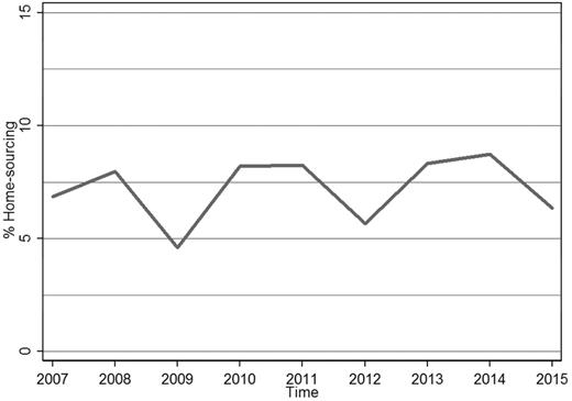
Home-sourcing dynamics across 2007–2015.
We can also observe the extent of home-sourcing across the different NACE industrial sectors, reported in Table 3. The share of home-sourcing activities is lower for low-technology sectors such as meat products, printing or beverages. Conversely, higher values are associated with industries defined by higher R&D intensity and input quality.12 These include chemicals and pharmaceuticals as well as computers and electronics. Similar to previous studies focusing on reshoring (Dachs and Kinkel, 2013), vehicles and transport equipment sectors present the highest share. When considering variation across firm size, we observe home-sourcing across the whole period to be higher among large firms (>250 employees), at 11%, as opposed to small firms (≤250 employees), with 6.5%.
% of Home-sourcing at industry level
| NACE sector | % Home-sourcing |
|---|---|
| 1. Meat products | 2.69 |
| 2. Food and tobacco | 5.74 |
| 3. Beverage | 5.88 |
| 4. Textiles and clothing | 6.83 |
| 5. Leather, fur and footwear | 7.27 |
| 6. Timber | 6.94 |
| 7. Paper | 8.59 |
| 8. Printing | 5.15 |
| 9. Chemicals and pharmaceuticals | 10.73 |
| 10. Plastic and rubber products | 7.87 |
| 11. Nonmetal mineral products | 5.2 |
| 12. Basic metal products | 8.8 |
| 13. Fabricated metal products | 4.74 |
| 14. Machinery and equipment | 8.05 |
| 15. Computer products, electronics and optical | 8.61 |
| 16. Electric materials and accessories | 8.56 |
| 17. Vehicles and accessories | 12.56 |
| 18. Other transport equipment | 10.14 |
| 19. Furniture | 7.42 |
| 20. Other manufacturing | 11.71 |
| Total | 7.16 |
4. Results and discussion
Results for the regression analysis are reported in Table 4. Overall, the statistically significant coefficients for our key variables of interest, reflecting R&D intensity and product standardization, offer support for both the hypotheses presented in the paper, suggesting that companies that engage in innovative and advanced manufacturing activities, characterized by higher R&D intensity and customized production, are more likely to home-source their activities, ceteris paribus. The opposite holds true for firms more reliant on labour-intensive activities. In particular, home-sourcing decisions are positively and significantly related to firms’ R&D intensity. This suggests that firms whose manufacturing activities require higher levels of innovation and technological knowledge may have more incentives to bring their value chain closer due to the positive effects of reduced time distance costs, which increase for knowledge-intensive interactions, and the innovation spillovers related to spatial embeddedness (Bathelt and Glückler, 2003; Becattini et al., 2009). This is also reflected in the positive coefficient for labour productivity, usually associated with high-end and technology-intensive production in manufacturing, which points to a higher productivity of domestic suppliers as a determinant of home-sourcing.
GEE and ML logit regression for panel data
| Home-sourcing | GEE | ML logit | ||||||
|---|---|---|---|---|---|---|---|---|
| B | Robust SE | B | Robust SE | B | Robust SE | B | Robust SE | |
| R&D intensity | 3.786** | (1.584) | 3.835** | (1.625) | 3.828** | (1.616) | 3.905** | (1.663) |
| Labor intensity | –3.483*** | (0.463) | –3.548*** | (0.468) | ||||
| Labor productivity | 0.400*** | (0.066) | 0.412*** | (0.067) | ||||
| Product standardization | –0.176* | (0.098) | –0.195** | (0.098) | –0.178* | (0.099) | –0.197** | (0.099) |
| Frequency product change | 0.164 | (0.164) | 0.190 | (0.164) | 0.165 | (0.167) | 0.192 | (0.167) |
| Capital intensity | –0.009 | (0.037) | –0.017 | (0.037) | –0.008 | (0.038) | –0.016 | (0.038) |
| Firm age | 0.001 | (0.002) | –0.000 | (0.002) | 0.001 | (0.002) | –0.000 | (0.002) |
| Firm size | 0.636*** | (0.162) | 0.680*** | (0.162) | 0.646*** | (0.162) | 0.690*** | (0.162) |
| Firm size^Firm size | ||||||||
| Market dynamics | –0.002 | (0.001) | –0.002 | (0.001) | –0.002* | (0.001) | –0.002 | (0.001) |
| N. international markets | 0.055 | (0.041) | 0.055 | (0.041) | 0.056 | (0.041) | 0.056 | (0.041) |
| % increase input costs | 0.101 | (0.746) | 0.294 | (0.732) | 0.111 | (0.754) | 0.305 | (0.742) |
| % increase energy costs | –0.419 | (0.873) | –0.399 | (0.875) | –0.383 | (0.882) | –0.361 | (0.886) |
| Constant | –4.387*** | (0.665) | –9.819*** | (0.852) | –4.492*** | (0.672) | –10.093*** | (0.863) |
| Industry dummies | Yes | Yes | Yes | Yes | ||||
| Year dummies | Yes | Yes | Yes | Yes | ||||
| Wald chi | 276.94*** | 253.01*** | 278.09*** | 253.80*** | ||||
| Log-likelihood | –2185.84 | –2197.47 | ||||||
| N firms | 1935 | 1935 | 1935 | 1935 | ||||
| Obs | 8359 | 8360 | 8359 | 8360 | ||||
* p ≤ 0.10 ** p ≤ 0.05 *** p ≤ 0.01—robust standard errors reported
In line with our second hypothesis, we also find that the decision to home-source is more likely to be taken in firms whose products are not standardized, namely where personalization and customization matter. This also supports those arguments stressing the importance of the ‘resilience’ of the supply chain and the increasing importance in the interactions required by innovative and customized production. Conversely, companies operating in markets characterized by standardized products and more dependent on labour cost efficiency are less likely to home-source intermediate inputs.
Our findings provide robust evidence in favour of closer value chains, suggesting in turn that the possibilities for (and impact of) home-sourcing has been underestimated. While home-sourcing may not create as many jobs as policymakers have hoped for, the fact that (in the Spanish case at least) companies with higher R&D intensity are more likely to home-source their activities than firms more reliant on labour intensity suggests that home-sourcing may ‘bring back’ and secure high-quality, high-productivity jobs, which in turn can ‘anchor’ other manufacturing and related service sector jobs.13 Overall, this suggests that the possible contribution of home-sourcing may be understated by those who have simply focused on the numbers of possible jobs it might create. Furthermore, we also find that the decision to home-source is more likely to be taken in firms whose products are not standardized, namely where personalization and customization matter, in line with the characteristics embodied in the new ‘distributed manufacturing’. Conversely, companies operating in markets characterized by standardized products and more dependent on labour cost efficiency are less likely to home-source intermediate inputs.
Interestingly, we also find evidence of an inverted-U relationship between home-sourcing and firm size, suggesting that outsourcing activities of the smaller firms may be linked with cost-saving decisions that are difficult to reverse. As size increases, medium-sized firms may have more capabilities to respond more dynamically to changes in demand and have a closer relationship with their supply chain. Larger firms may have more established and globalized production structures and may be less flexible in this sense. The inverse U-shaped relationship between firm size and home-sourcing mirrors previous descriptive evidence for other countries (Dachs and Zanker, 2014), with the inflection point calculated at mean values around the 92nd percentile of the firm size distribution corresponding to a threshold just below 500 employees, the 8% largest firms in the sample. This suggests that it may be medium-sized firms which may be more likely to home-source sourcing; policymakers taking an interest in home-sourcing to promote a more balanced economy with a strong manufacturing sector perhaps need to consider policy interventions focused more on medium-sized R&D-intensive manufacturing firms—in line with recent debates on the importance of mid-sized firms (the ‘mittelstand’) in some countries.
Splitting the data between large and small or medium companies, as well as high-tech and low-tech companies, offers further evidence for these findings. Results are reported in Table 5, presenting respectively estimates for small and large firms as well as high-tech and low-tech companies, defined by R&D intensity either above or below sector-level median values. We find R&D intensity to be significant only in the regression for large firms, which reflects the higher propensity to formal R&D in this group, while the effect of product standardization is significant only for SMEs. This may indeed reflect the relatively higher importance of proximity to customers for these firms. Furthermore, in line with the argument of a key relationship between high-quality and advanced production and home-sourcing, no evidence is found for these determinants across low-tech firms, while both R&D intensity and product standardization retain a significant effect for high-tech firms.
GEE logit regression for: (1) small and (2) large firms, (3) high-tech and (4) low-tech firms
| Home-sourcing | GEE | |||||||
|---|---|---|---|---|---|---|---|---|
| small | large | high tech | low tech | |||||
| B | Robust SE | B | Robust SE | B | Robust SE | B | Robust SE | |
| R&D intensity | 1.303 | (2.165) | 8.656*** | (2.886) | 3.344** | (1.649) | 7.278 | (5.573) |
| Labor intensity | –4.016*** | (0.509) | –1.142 | (1.150) | –2.899*** | (0.585) | –4.389*** | (0.729) |
| Product standardization | –0.181* | (0.108) | –0.284 | (0.260) | –0.253** | (0.125) | –0.056 | (0.158) |
| Frequency product change | 0.218 | (0.186) | –0.085 | (0.408) | 0.039 | (0.212) | 0.362 | (0.250) |
| Capital intensity | –0.019 | (0.040) | 0.010 | (0.099) | –0.031 | (0.047) | 0.011 | (0.059) |
| Firm age | 0.002 | (0.003) | –0.002 | (0.003) | –0.001 | (0.003) | 0.003 | (0.003) |
| Firm size | 0.211*** | (0.053) | –0.049 | (0.125) | 0.346* | (0.198) | 0.826*** | (0.279) |
| Firm size^Firm size | –0.034 | (0.021) | –0.065 | (0.030) | ||||
| Market dynamics | –0.003* | (0.002) | –0.003 | (0.003) | –0.002 | (0.002) | –0.002 | (0.002) |
| N. international markets | 0.063 | (0.050) | –0.006 | (0.069) | 0.073 | (0.050) | 0.044 | (0.068) |
| % increase input costs | 0.474 | (0.847) | –1.014 | (1.830) | –0.646 | (1.011) | 1.008 | (1.299) |
| % increase energy costs | –1.018 | (1.003) | 2.255 | (1.930) | 1.084 | (1.235) | –1.912 | (1.300) |
| Constant | –3.512*** | (0.634) | –2.566* | (1.476) | –2.480*** | (0.819) | –5.160*** | (0.999) |
| Industry dummies | Yes | Yes | Yes | Yes | ||||
| Year dummies | Yes | Yes | Yes | Yes | ||||
| Wald chi | 277.25*** | 681.54*** | 89.04*** | 191.46*** | ||||
| N firms | 1661 | 357 | 955 | 1040 | ||||
| Obs | 6979 | 1363 | 3958 | 4401 | ||||
* p ≤ 0.10 ** p ≤ 0.05 *** p ≤ 0.01—robust standard errors reported
5. Conclusions and policy implications
The paper weaves together literatures on international business, economic geography and global value chains to reach a better understanding of manufacturing reshoring, considering in particular the case of ‘home-sourcing’. The possibility of mature economies to be an attractive location for manufacturing activities offers an opportunity for renewal via a recoupling of innovation and production in the home economy. Critically, we argue that the interplay between the national and the global scales is being redefined in the context of a new competitive environment where the relative importance of scale economies versus variety is altered, and a recoupling between innovation and production in the same geographical space becomes more desirable.
Given that we wanted to test what would drive firms’ home-sourcing decisions, we argue that new configurations of outsourcing patterns can more quickly be adapted than long-term FDI decisions. Using a firm-level panel dataset containing information on the population of manufacturing companies in Spain for the period 2007–15 to explore firms’ decision on the location of their suppliers of intermediate inputs, we find that labour-intensive businesses are less likely to engage in home-sourcing, whereas R&D-intensive businesses with core non-standardized products are positively associated with home-sourcing.
These findings suggest some implications for industrial policymakers interested in encouraging home-sourcing. If the findings in the Spanish case are more generalizable, then policy in encouraging home-sourcing may have a role to play, but not in trying to bring back labour-intensive activities (these will anyway be susceptible to wage rate and exchange rate shifts and hence quite footloose in nature as relative unit labour costs shift). Rather, it is activities undertaken by R&D-intensive manufacturing firms producing non-standardised products that are more likely to be home-sourced. This may require something of a ‘mindset change’ on the part of policymakers and service providers who sometimes tend to equate ‘policy success’ with the numbers of jobs created or safeguarded, rather than the quality of such jobs, the value added they create and how long term and sustainable they actually can be.
We would therefore agree with De Backer et al. (2016) and Bailey and De Propris (2014) that home-sourcing (or for that matter reshoring) will not re-create large numbers of manufacturing jobs, and certainly not the low-skilled jobs that have been offshored or outsourced abroad. This means that industrial policymakers need to recognise that high-cost mature economies can be attractive for the location of R&D-intensive manufacturing functions for firms producing non-standardised products. Therefore, home-sourcing may indicate that high-quality jobs can be created in national manufacturing sectors in mature economies and may help boost firm performance through co-locating innovation and production. That in turn may help refine appropriate industrial policy instruments and expectations. Our findings suggest that the focus should be placed on the value creation content of the functions that are home-sourced (e.g. technology, competence, innovation) due to a multiplier effect that (a) creates or retains highly skilled jobs in manufacturing functions and (b) creates or anchors high-value services in the home economy. Overall the effect is of re-joining supply chain functions in the home national economy.
While home-sourcing is indeed a real opportunity, it is not a foregone conclusion, as its actual logistics can be challenging (Bailey and De Propris, 2014). In line with our theoretical framework, it should be noted that home-sourcing firms are not likely to be operating in isolation; rather, they will operate as part of ecosystems of firms. Whether it benefits mature economies will depend—inter alia—on the availability of skills, innovation capacity, the supply chain base, support services and the role of institutions. Maintaining an ecosystem of firms and agencies provides firms with a ‘deal-breaking’ anchor, making home-sourcing a viable option (this correlates to US and British reshoring experience; Bailey and De Propris, 2014). However, too much manufacturing supply chain ‘hollowing out’ will reduce such opportunities. In that regard, policy interventions should form part of a more holistic industrial strategy for stimulating business investment and new firm formation to rebuild national value and safeguard manufacturing ecosystem competitiveness in Europe. Policy needs to take this on board, for example in private-public-sector dialogue to identify opportunities to re-join supply chain functions. This would be in line with modern conceptions of industrial policy as a collaborative process of discovery of information (Bailey and De Propris, 2014; Bailey et al., 2015) involving the public and private sector (see Chang and Andreoni, 2014).
While the paper introduces a general framework for determinants of home-sourcing rooted in a recoupling of innovation and production in the same geographical space, and the increasing important of spatial embeddedness for advanced, innovative manufacturing, results from the empirical analysis should be interpreted taking into account some limitations inherent to the data available. In this sense, data limitations do not allow us to explicitly consider the specific characteristics of intermediate inputs and relative cost changes. Furthermore, additional data at the sub-national level are required to explore the regional effects of home-sourcing on the supply chain in the home country as well as the specific role of regional clusters. These elements certainly represent valuable avenues for further research.
Acknowledgements
The writing of this paper has been supported by the EU Horizon 2020 project MAKERS—Smart Manufacturing for EU growth and prosperity is a project funded by the Horizon 2020 Research and Innovation Staff Exchange Programme, which is a Research and Innovation Staff Exchange under the Marie Sklodowska-Curie Actions, grant agreement number 691192. Ethical disclaimer: the secondary data used in the paper was collected before the MAKERS project.
Footnotes
It should be stressed that multiple factors determine the distribution of value along the chain.
See Lorentz et al. (2016) on the challenges of managing a geographically dispersed supply base.
See, for instance, the breakdown in the auto value chains of Japanese multinationals after the earthquake (Bentley et al., 2013).
This is pertinent in industries such as automotive (Bailey et al., 2010).
See the debate on user-led innovation (Von Hippel, 2005).
It should be noted that ‘customised’ does not mean local demand only but rather high-value-added outputs where the customer co-creates the product with the producer requiring a more localised supply chain to produce bespoke products. See for example Singh Srai and Ané (2016) on how ‘end-users are demanding more responsive near-to-market supply chains’, with firm network reconfiguration and restructuring requiring continuous reappraisal of location decisions.
Equally, the ‘servitisation’ of manufacturing and a shift to a hybrid model where manufacturing and services are increasingly intertwined require a recoupling and closeness (De Backer et al., 2016).
See Boix (2009).
More information on the data and access to the questionnaire are available on the Fundación SEPI website, www.fundacionsepi.es.
Results are fully robust to variables calculated yearly.
One of the main strengths of GEEs is a consistent and unbiased estimation despite possible misspecification of the correlation structure (Hardin and Hilbe, 2013). In this study, the exchangeable correlation structure was selected following the quasi-likelihood independence criterion (QIC). See Pan (2001).
This is consistent with some recent studies on reshoring; see for example Heikkilä et al. (2018) on Nordic experience.
This has resonance with the work of Verdu et al. (2012), who analyse the evolution of firms’ offshore–inshore strategies in a footwear industry cluster in Spain; they find that while some firms have offshored production, others use proximity to the customer as a competitive weapon to create value by responding to consumers more rapidly.
