Optimal Income Tax in an Extensive Labor Supply Life-cycle Model

Abstract

This article considers a stationary economy populated with overlapping generations that reproduce identically in continuous time. Each dynasty has a productivity and an opportunity cost of going to work that vary with age. Labor supply is extensive. At each date, the typical agent can either work full time or not work at all. The decision to work is based on a comparison between after tax income and the privately known opportunity cost of work. We assume that the utilitarian government, which aims at redistributing lifetime utility across dynasties, has a single policy instrument, a stationary income tax schedule function of current income. The article develops a method to study the government problem. This technique is applied to derive the properties of the optimal income tax schedule in a number of examples.

1. Introduction

We study income taxation in a dynamic stationary economy with overlapping generations, made of dynasties with fixed lifetime that reproduce identically. Time is continuous. Labor supply is extensive. At each date, one can either work full time or not work at all. The typical agent is characterized by an invariant instantaneous utility function for consumption and deterministic profiles of productivity, that is, production when working full time, and pecuniary cost of going to work. For simplicity, we assume that these profiles are deterministic. The government aims at redistributing lifetime welfare across dynasties, using the income tax. We put a number of restrictions on the government instrument, based on casual observation of developed economies: we suppose that the tax schedule is invariant over time and that tax depends only on current labor income. It cannot depend on the pecuniary cost of going to work, which is implicitly not verifiable by the tax authority. All non-workers are identically treated (they pay the same amount or receive the absolute value of the transfer if tax is negative). This transfer is independent of the (potential) productivity, supposed not to be verifiable for non-working individuals. We derive the properties of the optimal tax system in this setup.

Its dynamic structure makes the article unlike the bulk of the optimal taxation literature that takes place in a static model; see, for example, the survey of Piketty and Saez (2013). Also, it is different from the intensive labor supply models that follow Mirrlees, where the agents only differ by their productivities along a single dimension of heterogeneity. It shares features of the extensive model, notably the heterogeneity in the cost of going to work, which may generate an optimal subsidy of the labor supply of the low-skilled agents as in Choné and Laroque (2005).

The dynamic setup is similar (overlapping generations, deterministic trajectories,…) to that used by a number of recent works, Rogerson (2011), Shourideh and Troshkin (2012), or Weinzierl (2011). Our contribution with respect to these studies is in our focus on the extensive margin and the treatment of the two-dimensional heterogeneity on productivity and the cost of going to work.

To be able to derive the properties of the optimal tax system, we rule out tax schemes that depend on the history of earnings, an assumption which we feel justified by casual observation. This makes our analysis very different from that of Brito et al. (1991) and more recently the dynamic public finance literature; see, for example, Kocherlakota (2005, 2010). These works are interested in the dynamic revelation of information. We stick to a simpler redistributive problem where the nonlinear tax is constrained to be a function of current income. We also do not allow income tax to depend on age, contrary to Weinzierl (2011). Again our justification is casual observation. A natural way to have transfers conditional on age would be to introduce pensions. This is outside the scope of the current article and should be the subject of future work.

The main contribution of the article is our characterization of the optimal tax scheme in this dynamic extensive labor supply environment. Indeed, the optimal tax can be described as the result of a balance between two forces: a redistributive force, holding labor supply constant, and an efficiency force, which comes from changes in labor supply and production. This generalizes the first-order conditions from Laroque (2011). There is a lot of bunching at the optimum: the tax scheme often is piecewise constant, and there are regions where the marginal tax rate is 100%. This is due to the extensive character of labor supply: what is important is whether to work or not to work, the average and not the marginal tax rate. Otherwise the model is too general to lead by itself to definite policy implications. Given the trajectories of the productivity and opportunity cost of work of the dynasties in the economy, given also the tastes for redistribution of the government, our analysis allows to compute the optimal tax schedule. Without further restrictions on the parameters of the economy, the tax schedule however is largely unconstrained. An interesting feature, for policy purposes, is the treatment of low-skilled agents whose labor supply may be distorted downward as in the traditional Mirrleesian intensive models or distorted upward, justifying the American Earned Income Tax Credit (EITC) and the introduction of negative taxes.

We have investigated in more depth, economies with two types of agents. We show that the optimal allocation dramatically changes depending on the source of the heterogeneity. When the agents primarily differ by their opportunity costs of work, the income tax schedule solves a standard equity/redistribution trade-off with each of the two types of agents having their labor supply distorted downward. By contrast, when the agents primarily differ through their productivity, the tax schedule is used to subsidize low-skilled work, and hence generates upward labor supply distortions. The logic at work is reminiscent of Choné and Laroque (2011). Here, however, the mechanism comes from the low-skilled agent being the only one working at low productivities, due to the form of her life cycle trajectory, rather than to the shape of the distribution of the social weights in the population.

The article is organized as follows. Section 2 presents the model. Section 3 deals with optimal taxation, introducing the efficiency and redistributive forces. Finally, Section 4 studies in detail the properties of optimal tax in the case where there are two types of agents in the economy.

2. Model

We consider an economy in continuous time. All agents have the same life length, normalized to one. The types i of the agents belong to a set I. Agent of type i has a lifetime utility function of the form

\int_{0}^{1} u_{i} [c_{i} (a)] d a,

where

u_{i}

is an increasing concave function and

c_{i} (a)

denotes consumption at age a. Agent i, if she works at age a, produces at most

w_{i} (a)

units of a single homogeneous good. Going to work on the market, and therefore producing

w_{i} (a)

⁠, has an opportunity cost for the agent, for instance because it takes time otherwise devoted to family gardening or to childcare. This cost varies with age along the life of agent i. We assume that this dependence with respect to age is deterministic and known. Formally the opportunity cost to work of agent i is pecuniary, measured in units of good, and represented with the function

δ_{i} (a)

⁠.

The type of an agent is thus characterized by a couple of exogenous, nonnegative functions $(w_{i} (\cdot), δ_{i} (\cdot))$ defined on $[0, 1]$ and by the instantaneous utility index $u_{i} (\cdot)$ ⁠. The pair $(w_{i} (a), δ_{i} (a))$ as the age a varies determines a curve in the $(w, δ)$ space, which we call a ‘trajectory’. We assume that the functions $w_{i}, δ_{i}$ ⁠, and $u_{i}$ are differentiable. The economy potentially exhibits a lot of heterogeneity.

At each date t, for each i in I, the economy contains a continuum of agents of type i of all ages a in $[0, 1]$ ⁠; overtime the older agents die and are replaced by newborns of the same type. Cohort i has size $n_{i}$ ⁠, with $\sum_{I} n_{i}$ normalized to 1, and the economy is stationary. An ‘allocation’ specifies the nonnegative consumption $c_{i} (a)$ and the labor supply $ℓ_{i} (a)$ in {0, 1} of all types i along their lives.

Furthermore, we assume that there are perfect financial markets for transferring wealth across time, with a zero interest rate. The agents use these markets to smooth their consumption overtime, $c_{i} (a) = c_{i}$ independent of age. From now on, we restrict our attention to allocations where consumption is constant and equal to its aggregate value over the lifetime $c_{i}$ ⁠.

2.1 Feasibility

An allocation is ‘feasible’ if and only if total consumption does not exceed total output net of production cost:

\sum_{I} n_{i} c_{i} \leq \sum_{I} n_{i} \int_{0}^{1} [w_{i} (a) - δ_{i} (a)] ℓ_{i} (a) d a .

(1)

An allocation is ‘efficient’ whenever output net of production costs is maximized, that is, any agent works whenever her opportunity cost of work is lower than or equal to her productivity,

ℓ_{i} (a) = 1

δ_{i} (a) < w_{i} (a)

and

ℓ_{i} (a) = 0

δ_{i} (a) > w_{i} (a)

⁠.

2.2 Utilitarian optimum (first best)

The utilitarian optimum is the allocation that maximizes

\sum_{I} n_{i} u_{i} (c_{i})

subject to the feasibility constraint (1). It is the feasible efficient allocation such that marginal utilities are equal:

u'_{i} (c_{i}) = λ,

for all i in I.

2.3 Laissez-faire

The agents maximize their lifetime consumption

c_{i} = \int_{0}^{1} \max (0, w_{i} (a) - δ_{i} (a)) d a .

They decide to work whenever their productivity is larger than their opportunity cost of work,¹ so the laissez-faire equilibrium is efficient. In general, laissez-faire yields an allocation that differs from the utilitarian optimum.

‘In all of the article we suppose that the utilitarian government observes the employment status of the agents and, when they work, their productivity w. It never observes the pecuniary cost δ, which is private information.’

2.4 Income tax

We study redistributive taxation in a setup where the tax schedule is assumed to be age independent and time invariant. The tax schedule is made of a function R(w), the after-tax income of a worker with before tax wage w, and of a scalar s equal to the subsistence income of the non-workers.

2.5 Second-best program

Facing the tax schedule

(R (\cdot), s)

⁠, the consumer chooses her labor supply

ℓ (a)

⁠, so as to maximize her lifetime utility, that is,

c_{i} = \max_{ℓ} s + \int_{0}^{1} [R (w (a)) - δ_{i} (a) - s] ℓ (a) d a

where

ℓ (a)

belongs to {0, 1}.

Feasibility then can be written in two equivalent ways, either as a balanced government budget:

\sum_{I} n_{i} {\int_{0}^{1} [w_{i} (a) - R (w_{i} (a)) + s] ℓ_{i} (a) d a - s} \geq 0,

(2)

or as the equality of aggregate production and aggregate consumption:

\sum_{I} n_{i} {\int_{0}^{1} [w_{i} (a) - δ_{i} (a)] ℓ_{i} (a) d a - c_{i}} \geq 0.

(3)

The second best allocation maximizes the sum of utilities under the above constraints.

3. Optimal Income Tax

When an agent has productivity w at some date, her financial incentive to work is equal to $R (w) - s$ ⁠, which is to be compared with the opportunity cost of work δ. It is useful to represent the financial incentive to work in the same plan as the individual trajectories $(w (a), δ (a))$ ⁠. Hereafter, the ‘incentive schedule’ is the curve $(w, R (w) - s)$ as productivity varies. An agent works in regions where her trajectory is located below the incentive schedule, that is, her opportunity cost of work δ is smaller than the financial incentive to work $R (w) - s$ ⁠. Her work status changes at points where her trajectory crosses the incentive schedule.

Assuming that the agents can choose occupations requiring skills below their own ability, no one would choose an occupation whose required productivity belongs to a decreasing part of the function R, preferring to produce less and to earn a higher after-tax income. Formally, we can replace any function R with

\tilde{R} (w) = \max_{w' \leq w} R (w')

⁠. It follows that, without loss of generality, we limit our attention to functions R that are nondecreasing and assume that workers work at full productivity. Lifetime consumption of agent i is therefore given by

c_{i} = s + \int_{0}^{1} [R (w_{i} (a)) - δ_{i} (a) - s] ℓ_{i} (a) d a,

(4)

with

For notational simplicity, we do not mention the policy instruments R and s in the arguments of the labor supply functions

ℓ_{i}

⁠. The Lagrangian of the problem reduces to

ℒ = \sum_{I} n_{i} {u_{i} (c_{i}) + λ [Y_{i} (ℓ_{i}) - c_{i}]},

where

λ

is the multiplier of the government budget and

Y_{i} (ℓ_{i})

is agent i’s lifetime net output:

Y_{i} (ℓ_{i}) = \int_{a = 0}^{1} [w_{i} (a) - δ_{i} (a)] ℓ_{i} (a) d a .

The problem is to find the tax instruments

(R (\cdot), s)

which maximize the Lagrangian

ℒ

subject to the constraint that

R (\cdot)

be nondecreasing. An equal translation of

R (\cdot)

and of the subsistence income s, which does not alter labor supply, yields the first-order necessary condition:

\sum_{I} n_{i} u_{i}' (c_{i}) = λ

⁠.

The Lagrangian depends on the tax schedule through two channels: consumption levels $c_{i}$ and labor supplies $ℓ_{i}$ ⁠. Hereafter, we label ‘redistribution force’ and ‘efficiency force’ the effect of R through these respective channels. The first force is present at all productivity levels, while the second is active only at points w where an agent is indifferent between working and not working. Formally, we compute the Fréchet derivatives of the Lagrangian of the government problem, seen as a functional that maps the set of functions R into $R$ ⁠. To this aim, we evaluate the Lagrangian at a slightly perturbed function $R + ɛ h$ ⁠, compute the ratio $[ℒ (R + ɛ h) - ℒ (R)] / ɛ$ ⁠, and let $ɛ$ tend to zero. A mathematical derivation of the limit can be found in Appendix A. Here we present a heuristic approach of the differentiation.

3.1 The redistribution force

This force comes from the dependence of lifetime consumptions on the after-tax schedule. Suppose we replace the after-tax income R with

R + d R

on the interval

[w, w + d w]

⁠, with

d w > 0

⁠. This change in after-tax income translates into a change in consumption for the agents who work at productivity levels in

[w, w + d w]

⁠. The change in agent i’s lifetime consumption is given by

d c_{i} = d T_{i} (w; ℓ_{i}) d R,

(5)

where

T_{i} (w; ℓ_{i})

denotes the time spent by agent i with worktime profile

ℓ_{i}

working in a productivity lower than or equal to w

T_{i} (w; ℓ_{i}) = \int_{0}^{1} ℓ_{i} (a) 1_{w_{i}} (a) \leq w d a,

(6)

and, accordingly, its derivative

d T_{i} (w; ℓ_{i})

represents the time spent by agent i working in a productivity between w and

w + d w

⁠.

By construction, $T_{i} (w; ℓ_{i})$ is a nondecreasing function of w. The limit of $T_{i} (w; ℓ_{i})$ as w goes to infinity is the total time agent i works over her life cycle, hereafter denoted $L_{i}$ ⁠.

The derivative of $T_{i} (w; ℓ_{i})$ with respect to w, $d T_{i} (w; ℓ_{i})$ ⁠, is a positive measure which is almost everywhere continuous, possibly having mass points at productivity levels where agent i spends non-infinitesimal periods of time. If we think of agent i’s productivity when she works as a random variable, the probability measure $d T_{i} (w; ℓ_{i}) / L_{i}$ can be thought of as the distribution of that random variable. Suppose agent i’s trajectory crosses the incentive schedule from below at w₀, that is, the agent works for $w \leq w_{0}$ and does not work for $w \geq w_{0}$ along the trajectory. Then $d T_{i}$ has a downward discontinuity at w₀, and $T_{i}$ has a concave kink at w₀. If the trajectory crosses the schedule from above, then the kink of $T_{i}$ is convex.

By the chain rule, the variation of the Lagrangian coming from the changes in lifetime consumptions is given by

dℒ = d Φ (w; ℓ)

⁠, where

Φ (w; ℓ)

is the social marginal utility of income (net of the cost of public funds) for workers with productivity below w:

Φ (w; ℓ) = \sum_{I} n_{i} [u'_{i} (c_{i}) - λ] T_{i} (w; ℓ_{i}) .

(7)

The term

d Φ (w; ℓ)

reflects the redistributive force. Redistribution induces the government to raise (lower) after-tax income in regions where

d Φ (w; ℓ) > 0

(⁠

d Φ (w; ℓ) < 0

⁠). The observation that λ is the average of marginal utilities yields the following result.

Lemma 1. The net social marginal utility of income of workers with productivity below w, $Φ (w; ℓ)$ ⁠, has the same sign as the correlation between marginal utilities $u'_{i} (c_{i})$ and working times $T_{i} (w; ℓ_{i})$ ⁠.

3.2 Labor supply elasticity

A change in the tax schedule may also affect labor supply. We say that there is ‘indifference’ at w if there exists an agent i, having productivity w at some age

a_{i}, w = w_{i} (a_{i})

⁠, who is indifferent between working and not working at this age, that is,

R (w) - δ_{i} (a_{i}) = s

⁠. A ‘switch point’ is an indifference point such that the work status of the indifferent agent changes in a neighborhood of w, that is, the trajectory of agent i crosses the incentive schedule at w. When the slopes of the tax schedule and of the trajectory are different,

R' (w) \neq δ_{i}' / w'_{i}

⁠, the quantity

η_{i} (w; R) = \frac{1}{| δ'_{i} (a_{i}) - R' (w) w_{i}' (a_{i}) |}

(8)

is positive and finite.

Consider a switch point w and replace R with

R + d R

on the interval

[w, w + d w]

⁠, with

d R = (δ_{i}' / w'_{i} - R') d w

⁠, as shown on Figure 1. (In the represented example, the trajectory is decreasing in the

(w, δ)

space; specifically the agent’s productivity and cost of work, respectively, decline and rise with age.) The perturbation changes the status of the agent on the interval from working to non-working. The time spent in the interval is

d a = d w / | w'_{i} | = η_{i} d R,

hence,

η_{i}

is the absolute value of the derivative of labor supply with respect to the tax schedule R. When R – s increases by 1%, the time agent i spends working at a productivity below w is increased by

ɛ_{i} (w; R)

percent, where

ɛ_{i} (w; R)

denotes the elasticity of agent i’s labor supply,

T_{i} (w; ℓ_{i})

⁠, with respect to financial incentives to work:

ɛ_{i} (w; R) = \frac{R (w) - s}{T_{i} (w; ℓ_{i})} η_{i} (w; R) .

(9)

The labor supply elasticity depends on both the gradient of the trajectory and the slope of the after-tax schedule at the switch point. In particular, the steeper the tax schedule at w, the lower the elasticity, because the agent spends less time in the region affected by the perturbation.

Figure 1

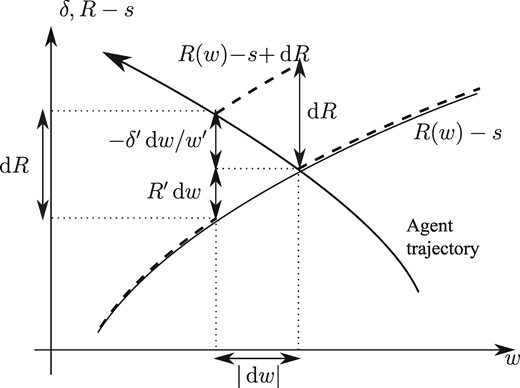
Labor supply elasticity. Original (perturbed) schedule: solid (dashed) line.

Open in new tab Download slide

The above formula is readily adapted if agent i’s trajectory crosses the tax schedule more than once. Formally, the Fréchet-derivative of

T_{i} (w; ℓ_{i})

with respect to the tax schedule R is a positive measure made of mass points at agent i’s switch points below w, see equation (16) in Appendix A.2. Similarly, the elasticity of the aggregate labor supply,

T (w; ℓ) = \sum_{I} n_{i} T_{i} (w; ℓ_{i})

⁠, is given by

ɛ (w; R) = \frac{R (w) - s}{T (w; ℓ)} \sum_{S (w)} n_{i} η_{i} (w; R),

(10)

where

S (w)

is the set of agents who switch at w.

3.3 The efficiency force

A marginal change of the incentives to work,

d (R - s)

⁠, on a small interval around a switch point w of agent i has only a second-order effect on her permanent income because she is indifferent between working and not working at this point. Such a change, however, affects the net output she produces over her life cycle:

d Y_{i} (ℓ_{i}) = [w - δ] η_{i} (w; R) d R,

(11)

where

δ = R (w) - s

is agent i’s cost of work at the switch point. At the same time, the change affects the government revenue. For instance, if

d R > 0

and

w > R - s

⁠, the variation of the tax schedule induces the agent to switch from not working to working on a short period of her life, which raises the government revenue. We define the efficiency force as

d Ψ (w; ℓ) = λ \sum_{I} n_{i} d Y_{i} (ℓ_{i}) .

We show formally in Appendix A that this force is a discrete measure concentrated on the set of all switch points

Ψ (w; ℓ) = λ \sum_{σ \in S} n_{i} [w_{σ} - R (w_{σ}) + s] η_{i} (w_{σ}; R) 1_{w_{σ}} \leq w,

(12)

where

S

is the set of all agents’ switch points,

w_{σ}

is the productivity level at

σ

⁠, and

ɛ (w; R)

is the total labor supply elasticity given by (10). The previous analysis is summarized in the following proposition.

Proposition 1. The Lagrangian

ℒ

is differentiable at any point

(w, R (w) - s)

where no trajectory is tangent to the incentive schedule. Its derivative can be written as the sum

dℒ = d Φ (w; ℓ) + d Ψ (w; ℓ),

(13)

where the almost everywhere continuous measure

d Φ (w; ℓ)

given by (7) and the discrete measure

d Ψ (w; ℓ)

given by (12) represent the redistribution and efficiency forces.

Raising R at an indifference point increases labor supply, which alleviates the government budget constraint if $w > R - s$ and makes it more stringent if $w < R - s$ ⁠. Hence, income maximizing pushes the government to raise (lower) after-tax income in regions where $w > R - s$ (⁠ $w < R - s$ ⁠). This force translates into mass points in the derivative of the Lagrangian or even into discontinuity points in the Lagrangian function.

On the other hand, the redistributive force, expressed in the term (7), is absolutely continuous (except at productivity levels where some workers spend a finite time): the redistributive effect of an increase in the after-tax income on an interval of productivities is the integral on the interval of the net social marginal utility of income $d Φ$ ⁠.

3.4 Finite number of types

The above analysis allows to concentrate attention on a particular class of tax schedules when I is finite:

‘When the number of types is finite, the second-best optimum may be implemented with an incentive schedule that is piecewise either constant or coincident with an increasing trajectory.’

The proof is in Appendix B. When the tax schedule coincides with an increasing trajectory, the government faces a particularly strong efficiency force.² Otherwise, the monotonicity constraint binds. Putting the signs of

d Φ (w; l)

and

d Ψ (w; l)

on the diagram of trajectories allows to qualitatively separate intervals of productivities where the redistribution and efficiency forces tend to push R up from those where these forces are downward.

Since we expect bunching to be the norm, it is worthwhile to spell out the form of first-order conditions under bunching. Consider a bunching interval

[w_{0}, w_{1}]

⁠. We can raise or lower R on the whole bunching interval, raise it on right subintervals

[w, w_{1}]

⁠, and lower it on left subintervals

[w_{0}, w]

⁠. None of these variations should increase the Lagrangian, which yields the first-order conditions:

dℒ ([w, w_{1}]) \leq 0,

(14)

for all w in the interval, with equality for w = w₀. This implies in particular that

dℒ

is nonnegative at w₀ and non-positive at w₁.

4. An Example: Two Types and Decreasing Trajectories

The results of the previous analysis greatly simplify the computation of the optimal tax schedule in economies covered by our assumptions. We can derive stronger analytical results when the environment is simpler. In practice, in this last section, we consider economies with two types of agents, a high type H and a low type L, endowed with the same utility function u. To adapt arguments based on incentives, we need the trajectories to be single crossing, which pushes us to focus on the second parts of lives, when productivity decreases with age while the opportunity cost of work increases with age. We also need the two types to be unambiguously ranked, the high type being more productive on the market and with a smaller opportunity cost of work than the low type, at all ages:

w_{H} (a) > w_{L} (a)

and

δ_{H} (a) < δ_{L} (a)

for all a in

[0, 1]

⁠. We also suppose that there is a natural retirement age: the trajectories intersect the 45 degree line.³

Figure 2.

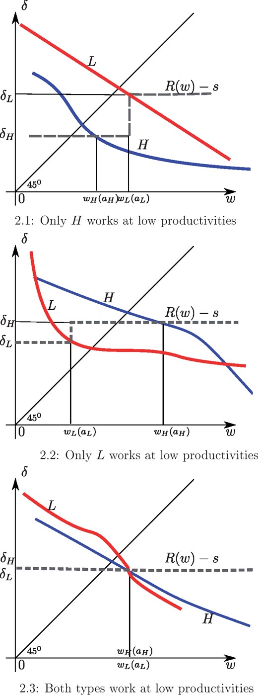
The three cases of Proposition 2.

Open in new tab Download slide

This set of assumptions is consistent with many different patterns. If the agents’ productivities are very close while their opportunity costs of work are very different, agent L’s trajectory is above agent H’s in the

(w, δ)

plan; see Figure 3. In the opposite case, agent H trajectory lies at the right of that of agent L; see Figure 4. The trajectories may very well cross, possibly many times, meaning that the same characteristics (productivity, cost) are reached by the two agents at different ages. Formally, the following properties hold.

Assumption 4.1 (Decreasing trajectories). The two agents have the same utility functions u. Their productivities, $w_{H} (a) > w_{L} (a)$ ⁠, decrease with age and their pecuniary costs of work, $δ_{H} (a) < δ_{L} (a)$ ⁠, increase with age. There exist ages $a_{L}^{*}$ and $a_{H}^{*}$ in (0, 1) such that $w_{L} (a_{L}^{*}) = δ_{L} (a_{L}^{*})$ and $w_{H} (a_{H}^{*}) = δ_{H} (a_{H}^{*})$ ⁠.

Figure 3.

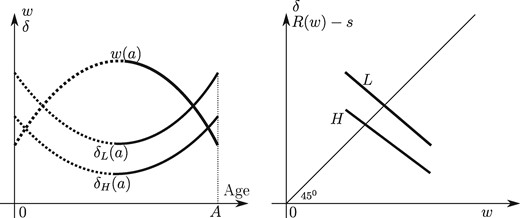
Two types, same productivities.

Open in new tab Download slide

Figure 4.

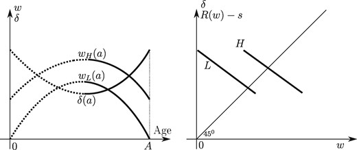
Two types, same opportunity costs of work.

Open in new tab Download slide

The fact that type H dominates pointwise type L implies that its consumption and welfare are at least as large, whatever the tax schedule,

c_{H} \geq c_{L}

⁠. Any nondecreasing tax schedule crosses each trajectory only once, respectively, at ages a_H and a_L,

a_{H} \geq a_{L}

⁠, with associated wages

w_{H} (a_{H})

and

w_{L} (a_{L})

and opportunity costs of work

δ_{H} (a_{H})

and

δ_{L} (a_{L})

⁠. The wages

w_{H} (a_{H})

and

w_{L} (a_{L})

represent the lowest productivities at which the agents work. The following proposition, whose proof is in Appendix C, provides the list of all possible configurations at the second-best optimum. Then we present two examples that illustrate how unobserved heterogeneity affects the labor supply distortions.

Proposition 2. Under Assumption 4.1, the following properties hold:

There exists an optimal tax schedule with at most two values;
Agent H has her labor supply distorted downward;
Agent L labor supply can be distorted in any direction or undistorted;
Agent H retires later and enjoys higher lifetime consumption than agent L:

c_{H} - c_{L} = \int_{0}^{a_{L}} [δ_{L} (a) - δ_{H} (a)] d a + \int_{a_{L}}^{a_{H}} [R (w_{H} (a)) - s - δ_{H} (a)] d a > 0.

(15)

We now illustrate the impact of the heterogeneity on labor supply distortions, see point (ii) and (iii) of Proposition 2. We use two examples where the agents differ only in one dimension, either productivity or opportunity cost of work. These examples, therefore, are at the limit of what is permitted by Assumption 4.1. Again, we focus on the second part of the agents’ lives where productivity decreases and opportunity cost of work increases, as in the solid lines of the left panels of Figures 3 and 4.

Example 1 (Same productivities, different opportunity costs of work). In addition to Assumption 4.1, suppose that the agents are equally productive, $w_{H} (a) = w_{L} (a)$ for all a, while agent H has a lower pecuniary cost of work: $δ_{H} (a) < δ_{L} (a)$ for all a. Then at the optimum, both agents have their labor supply distorted downward.

In Example 1, we must be in case (1) of the proof of Proposition 2. Moreover, the configuration with

δ_{L} (a_{L}) = δ_{H} (a_{L})

is not possible here. Indeed, as the two agents would work exactly the same time at productivities above any threshold w, an increase of the tax schedule above

w (a_{L}) - ɛ

for a small

ɛ > 0

would have no redistributive effect and a positive efficiency effect at

w (a_{L})

—a contradiction. The optimal schedule is therefore discontinuous at

w (a_{L})

as shown on the left panel of Figure 5.

Example 2 (Different productivities, same opportunity costs of work). In addition to Assumption 4.1, suppose that the agents have the same pecuniary costs of work, $δ_{H} (a) = δ_{L} (a)$ for all a, while agent H is more productive: $w_{L} (a) < w_{H} (a)$ ⁠. Then at the optimum, agent L has her labor supply distorted upward.

Figure 5

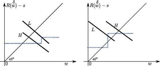
The optima with same productivities (left), same opportunity costs of work (right).

Open in new tab Download slide

In Example 2, we must be in case (2) of the proof of Proposition 2. Moreover, the configuration where the tax schedule is flat is not possible here. Indeed, the equality $δ_{L} (a_{L}) = δ_{H} (a_{L})$ would imply a_L = a_H, meaning that the two agents would have the same total working time: a uniform increase of R − s would thus have no redistributive effect and a positive efficiency effect at $w_{H} (a_{H})$ —a contradiction. The optimal schedule is therefore discontinuous at $w_{L} (a_{L})$ as shown on the right panel of Figure 5.

In Example 1, the heterogeneity primarily comes from the opportunity cost of work, while in Example 2, it comes from the productivity. In both cases, the government cannot implement the first best in these two-type economies. The direction of the distortions, however, is sensitive to the source of the heterogeneity.

1 Suppose that $δ_{i} (a)$ is a disutility cost instead of a pecuniary one, i.e. agent i, when working, produces $w_{i} (a)$ and has instantaneous utility $u (c_{i} (a)) - δ_{i} (a)$ ⁠, while she has instantaneous utility $u (c_{i} (a))$ when not working. Then agent i works at age a under laissez-faire if and only if $u_{i}' (c_{i}) w_{i} (a) > δ_{i} (a)$ ⁠, where $c_{i}$ is her constant, instantaneous consumption level. Hence, this specification entails an ‘income effect’ in labor supply: participation decreases with $c_{i}$ ⁠. Using Pareto-optimality conditions, it can be checked that laissez-faire is efficient. The pecuniary model adopted in this article avoids these complications.

2 See the last paragraph of Appendix B.

3 A referee has asked us to what extent the results below can be generalized. We certainly can have more than two types. But the monotony and ranking of the dynasties are an essential element of the argument.

4 In other words, the Lagrangian is locally discontinuous in productivity regions where the tax schedule is locally tangent to a trajectory, see Appendix A.2.

5 The first-order conditions imply that the net social marginal utility of income, $d Φ$ ⁠, is identically zero on $[w, w']$ and that $R (w) - s = w$ at any switch point in this region.

Appendix

A. Proof of Proposition 1

A.1 Derivative of lifetime consumption and redistribution force

We first compute the Fréchet-derivative of lifetime consumption levels with respect to the tax schedule R. We consider a perturbation

R + ɛ h

of the tax schedule, where h is a nonnegative test function h with compact support. Using the expression of

c_{i}

⁠, equation (4), and the change of variables

w = w_{i} (a)

⁠, we find that the ratio

[c_{i} (R + ɛ h) - c_{i} (R)] / ɛ

tends to

\int_{0}^{1} h (w_{i} (a)) ℓ_{i} (a) d a = \int h (w) d T_{i} (w; ℓ_{i})

ɛ

goes to zero, meaning that the positive measure

d T_{i} (w; ℓ_{i})

is the Fréchet-derivative of

c_{i}

⁠. This is the formal statement corresponding to equation (5).

T_{i} (w) / L_{i}

is the cumulative distribution function of

w_{i}

seen as a random variable. If we think of agent i’s productivity when she works as a random variable and denote that variable by

{\tilde{W}}_{i}

⁠, the above integral can be seen as the expectation of

h ({\tilde{W}}_{i})

⁠, multiplied by

L_{i}

⁠.

The chain rule then yields the redistribution force (7). Keeping labor supply constant, the ratio

[ℒ (R + ɛ h) - ℒ (R)] / ɛ

tends to

\sum_{I} n_{i} [u'_{i} (c_{i}) - λ] \int h (w) d T_{i} (w)

ɛ

goes to zero, which yields (7).

A.2 Labor supply elasticity and efficiency force

Labor supply is changed under the perturbed schedule $R + ɛ h$ only if the support of h contains switching points. For ease of exposition, we assume that the support contains only one switching point, that we denote by $\bar{w}$ ⁠. We denote by i the switching agent and by $a_{i}$ the age at which agent i switches at $\bar{w}$ ⁠. We have: $w_{i} (a_{i}) = \bar{w}$ and $R (\bar{w}) - s = δ_{i} (a_{i})$ ⁠. To fix ideas, we suppose that both $δ' (a_{i})$ and $w' (a_{i})$ are positive and that the slope of the indifferent agent’s trajectory is larger than the slope of the schedule: $δ_{i}' (a_{i}) / w' (a_{i}) > R' (\bar{w})$ ⁠.

The perturbed schedule

R + ɛ h

crosses agent i’s trajectory at points w such that there exists a with

w = w (a)

and

I (a, ɛ) = 0

⁠, where

I (a, ɛ) = ɛ h (w (a)) - δ (a) + R (w (a)) - s .

\partial I / \partial ɛ (a_{i}, 0) = h (\bar{w})

and

\partial I / \partial a (a_{i}, 0) = - δ_{i}' (a_{i}) + R' (\bar{w}) w_{i}' (a_{i})

⁠, the ratio

[T_{i} (w; R + ɛ h) - T_{i} (w; R)] / ɛ

tends to

{\begin{matrix} \frac{h (\bar{w})}{δ_{i}' (a_{i}) - R' (\bar{w}) w_{i}' (a_{i})} & for w > \bar{w} \\ 0 & for w \leq \bar{w} . \end{matrix}

ɛ

goes to zero. If the slope of the tax schedule is larger than that of the trajectory,

δ_{i}' (a_{i}) / w' (a_{i}) < R' (\bar{w})

⁠, replacing R with

R + ɛ h

changes labor supply on the left of

\bar{w}

and the ratio

[T_{i} (w; R + ɛ h) - T_{i} (w; R)] / ɛ

tends to

{\begin{matrix} \frac{h (\bar{w})}{| δ_{i}' (a_{i}) - R' (\bar{w}) w_{i}' (a_{i}) |} & for w \geq \bar{w} \\ 0 & for w < \bar{w} . \end{matrix}

ɛ

goes to zero. This yields expression (9) for the elasticity of agent i’s labor supply. The Fréchet derivative of

T_{i} (w; R)

is thus given by

\frac{\partial T_{i} (w; R)}{\partial (R - s)} = \sum_{σ \in S_{i} (w)} ɛ_{i} (w_{σ}; R) \frac{T_{i} (w_{σ}; R)}{R (w_{σ}) - s} ζ (w_{σ}),

(16)

where

S_{i} (w)

is the set of agent i’s switch points

σ

located below w,

w_{σ} \leq w

is the agent’s productivity at

σ

⁠, and

ζ (w_{σ})

denotes the mass point at

w_{σ}

⁠. The Fréchet derivative of the total labor supply T has the same expression as above, replacing

S_{i} (w)

with

S (w)

⁠, the set of ‘all’ agents’ switch points located below w.

We use the same method to compute the Fréchet derivative of the term $\int_{0}^{1} [w_{i} (a) - δ_{i} (a)] ℓ_{i} (a) d a$ ⁠. The only difference with the above analysis is the presence of the multiplicative term $w_{i} (a) - δ_{i} (a)$ ⁠, which, at $a = a_{i}$ ⁠, is equal to $\bar{w} - R (\bar{w}) + s$ ⁠, given that $\bar{w}$ is a switch point. This yields (12) and (13).

Discontinuous Lagrangian

Consider an indifference point w such that the incentive schedule is locally tangent to the indifferent agent’s trajectory. (In other words, we have: $σ = R'$ ⁠.) Then the Lagrangian is discontinuous at w, as an infinitesimally small increase in R implies a non-infinitesimal change in the Lagrangian. In other words, the efficiency force is particularly strong, creating a discontinuity in the Lagrangian, whose sign is the same as that of $w - R + s$ ⁠. This is in particular the case where the tax schedule locally coincides with an agent trajectory.

B. From Increasing to Piecewise Constant Schedules

Lemma B.1 Let R be any nondecreasing tax schedule. Let $\underset{̲}{w} < \bar{w}$ be such that none of the agents’ trajectories $(w_{i} (a), δ_{i} (a)), a \in [0, 1]$ ⁠, $i \in I$ ⁠, intersects the rectangle $[\underset{̲}{w}, \bar{w}] \times [R (\underset{̲}{w}), R (\bar{w})]$ ⁠. Assume that the functions $T_{i}$ have at most finitely many discontinuity points.

Then there exists a nondecreasing tax schedule

\bar{R}

⁠, such that

\bar{R}

is piecewise constant, with finitely many pieces, on

[\underset{̲}{w}, \bar{w}], \bar{R}

takes its values in

[R (\underset{̲}{w}), R (\bar{w})]

on this interval, and

\int_{\underset{̲}{w}}^{\bar{w}} \bar{R} (w) d T_{i} (w) = \int_{\underset{̲}{w}}^{\bar{w}} R (w) d T_{i} (w)

for

i \in I

⁠. If all the functions

T_{i}

are continuous on

[\underset{̲}{w}, \bar{w}]

⁠, then the schedule

\bar{R}

has at most #

I + 1

pieces on

[\underset{̲}{w}, \bar{w}]

⁠.

Proof. By assumption, labor supply is not affected as long as the schedule remains between

R (\underset{̲}{w})

and

R (\bar{w})

⁠. We can therefore drop the second argument in the functions

T_{i}

⁠, writing

T_{i} (w)

rather than

T_{i} (w, R)

⁠. Let

w_{1}, \dots, w_{N}

be the discontinuity points of the functions

T_{i}

⁠. Let

w_{0} = \underset{̲}{w}

and

w_{N + 1} = \bar{w}

⁠. We have:

\int_{\underset{̲}{w}}^{\bar{w}} R (w) d T_{i} (w) = \sum_{j} \int_{w_{j}}^{w_{j + 1}} R (w) d T_{i} (w) + R (w_{j}) [T_{i} (w_{j}^{+}) - T_{i} (w_{j}^{-})] .

It is sufficient to prove the result on each interval

[w_{j}, w_{j + 1}]

⁠. Integrating by parts yields:

\int_{w_{j}}^{w_{j + 1}} R (w) d T_{i} (w) = [T_{i} (w_{j + 1}^{-}) - T_{i} (w_{j}^{+})] R (w_{j + 1}) - \int_{w_{j}}^{w_{j + 1}} [T_{i} (w) - T_{i} (w_{j}^{+})] d R (w) .

We now apply Lemma A.1 (p. 1260) of Ghosal and Van der Vaart (2001) with the compact set

K = [w_{j}, w_{j + 1}]

⁠, the probability measure

F_{0} = d R (w) / [R (w_{j + 1}) - R (w_{j})]

and the functions

Ψ_{i} (w) = T_{i} (w) - T_{i} (w_{j}^{+}), i = 1, \dots, I

⁠, which are continuous on K. The Lemma yields a discrete probability measure ν on K with at most I + 1 support points such that

\frac{1}{[R (w_{j + 1}) - R (w_{j})]} \int_{w_{j}}^{w_{j + 1}} [T_{i} (w) - T_{i} (w_{j}^{+})] d R (w) = \int_{w_{j}}^{w_{j + 1}} [T_{i} (w) - T_{i} (w_{j}^{+})] d ν (w)

for all

i = 1, \dots, I

⁠. Integrating again by parts yields

\begin{array}{l} \int_{w_{j}}^{w_{j + 1}} R (w) d T_{i} (w) = [T_{i} (w_{j + 1}^{-}) - T_{i} (w_{j}^{+})] R (w_{j + 1}) \\ - [R (w_{j + 1}) - R (w_{j})] \int_{w_{j}}^{w_{j + 1}} [T_{i} (w) - T_{i} (w_{j}^{+})] d ν (w) \\ = [T_{i} (w_{j + 1}^{-}) - T_{i} (w_{j}^{+})] R (w_{j + 1}) \\ - [R (w_{j + 1}) - R (w_{j})] [T_{i} (w_{j + 1}^{-}) - T_{i} (w_{j}^{+})] \end{array}

\begin{array}{l} + [R (w_{j + 1}) - R (w_{j})] \int_{w_{j}}^{w_{j + 1}} ν (w) d T_{i} (w) \\ = \int_{w_{j}}^{w_{j + 1}} \bar{R} (w) d T_{i} (w) \end{array}

with

\bar{R} (w) = R (w_{j}) + [R (w_{j + 1}) - R (w_{j})] ν (w)

⁠. The schedule

\bar{R}

is nondecreasing and piecewise constant, with at most I + 1 pieces. It takes its values in

[R (w_{j}), R (w_{j + 1})]

⁠. □

Properties of the optimum when there is a finite number of types Consider an interval where the schedule is increasing. The schedule can locally coincide with an increasing trajectory, in which case efficiency and redistribution play in opposite directions: the schedule is slightly below the trajectory if $d Φ > 0$ and $w < R - s$ ⁠, slightly above if $d Φ < 0$ and $w > R - s$ ⁠. For instance, in the former case, lowering (raising) R entails an infinitesimal (a non-infinitesimal) fall in the Lagrangian through the redistribution (efficiency) effect.⁴

Now consider an interval $[w, w']$ where the schedule is increasing and does not coincide with an increasing trajectory.⁵ By compactness of $[w, w']$ ⁠, there exists a finite sequence $w = w_{1} < \dots < w_{h} = w'$ such that no trajectory crosses the rectangles $[w_{j}, w_{j + 1}] \times [R (w_{j}), R (w_{j + 1})]$ ⁠. On each interval $[w_{j}, w_{j + 1}]$ ⁠, we apply Lemma B.1 and replace R with a piecewise constant schedule that takes its values in $[R (w_{j}), R (w_{j + 1})]$ and leaves the government revenue and the agents’ lifetime consumption and labor supply unchanged.□

C. Proof of Proposition 2

Proof. The inequality a_H > a_L follows from the ordering and the monotonicity of the functions $R (w_{i} (a)) - s - δ_{i} (a), i = H, L$ ⁠. This inequality, in turn, implies c_H > c_L and $u' (c_{H}) < u' (c_{L})$ ⁠.

Consider any productivity threshold w greater than

\bar{w} = \max (w_{H} (a_{H}), w_{L} (a_{L}))

⁠. Only the redistribution force is present above w and its integral over the set

[w, w_{H} (0)]

⁠,

(u' (c_{H}) - λ) (T_{H} (w; l) - T_{H} (w_{H} (0); l) + (u' (c_{L}) - λ) (T_{L} (w; l) - T_{L} (w_{L} (0); l),

is strictly negative because

u' (c_{H}) < u' (c_{L})

and agent H spends strictly more time working in that region than agent L,

w_{H}^{- 1} (w) > w_{L}^{- 1} (w)

⁠. The function

r (w) = \min (0, R (\bar{w}) - R (w))

is non-increasing, and is an admissible variation of the tax schedule, as

R + ɛ r

is nondecreasing for small values of

ɛ

⁠. We must therefore have:

\begin{matrix} < dℒ, r > = \int_{\bar{w}}^{w_{H} (0)} r (w) d Φ (w; l) \\ = \int_{\bar{w}}^{w_{H} (0)} r' (w) [Φ (w_{H} (0); l) - Φ (w; l)] d w \leq 0. \end{matrix}

Since the bracketed term in the above inequality is negative and

r' \leq 0

⁠, we get

r' = 0

and thus

R (\bar{w}) = R (w)

⁠. The after-tax schedule, therefore, is flat above

\max (w_{H} (a_{H}), w_{L} (a_{L}))

⁠.

We now consider three cases in turn:

Agent H is the only one working at low productivities, $w_{H} (a_{H}) < w_{L} (a_{L})$ ⁠;
Agent L is the only one working at low productivities, $w_{L} (a_{L}) < w_{H} (a_{H})$ ⁠;
Both agents work at low productivities, $w_{H} (a_{H}) = w_{L} (a_{L})$ ⁠.

In case (1), only agent H works at productivities lying between

w_{H} (a_{H})

and

w_{L} (a_{L})

⁠. Since

u' (c_{L}) > u' (c_{H})

⁠, the redistribution force in that interval pushes downward, so the financial incentive to work R − s equals

δ_{H} (a_{H})

in that interval. From the bunching conditions, it must be the case that the efficiency force is active and upward at

w_{H} (a_{H})

⁠, hence

w_{H} (a_{H}) > δ_{H} (a_{H})

⁠: agent H’s labor supply is distorted downward.

To examine agent L’s labor supply, we suppose first the tax schedule is continuous at $w_{L} (a_{L})$ ⁠, that is, $δ_{L} (a_{L}) = δ_{H} (a_{H})$ ⁠. In this case, the after-tax schedule takes only one value for $w \geq w_{H} (a_{H})$ ⁠, namely the common value of $δ_{L} (a_{L}) = δ_{H} (a_{H})$ ⁠, and agent L’s labor supply is distorted downward because $w_{L} (a_{L}) - δ_{L} (a_{L})$ is larger than $w_{H} (a_{H}) - δ_{H} (a_{H}) > 0$ ⁠. We consider now the case where the schedule is discontinuous at $w_{L} (a_{L})$ ⁠. We know that R − s is flat and equal to $δ_{L} (a_{L})$ above that point. We can therefore consider a transformation that pushes R − s down from $δ_{L} (a_{L})$ to $δ_{H} (a_{H})$ just above $w (a_{L})$ ⁠. The redistribution and efficiency effects of the transformation respectively bear on type H and type L. The former is positive and of the sign of $(u'_{H} - λ) (δ_{L} - δ_{H})$ since it takes $δ_{L} - δ_{H}$ from type H while leaving L’s lifetime consumption level unaffected. The latter is of the sign of $- (w (a_{L}) - δ_{L})$ ⁠. For them to sum up to zero, we must have $w (a_{L}) > δ_{L} (a_{L})$ ⁠: agent L’s labor supply, again, is distorted downward.

In case (2), we have $δ_{H} (a_{H}) = R (w_{H} (a_{H})) - s \geq R (w_{L} (a_{L})) - s = δ_{L} (a_{L})$ ⁠. We deal separately with the situation where the two agents have the same opportunity costs when they stop working, and when that of H is larger than that of L. Suppose first that $δ_{L} (a_{L}) = δ_{H} (a_{H})$ ⁠. Then the financial incentive to work $R (w) - s$ is equal to that common opportunity cost for all $w \geq w_{L} (a_{L})$ ⁠. The efficiency force $w_{L} (a_{L}) - δ_{L} (a_{L})$ cannot be downward at $w_{L} (a_{L})$ as this would violate the first-order condition on the bunching interval starting at $w_{L} (a_{L})$ (in practice, the government would slightly decrease the after-tax income at $w_{L} (a_{L})$ ⁠), hence $w_{H} (a_{H}) > w_{L} (a_{L}) \geq δ_{L} (a_{L}) = δ_{H} (a_{H})$ ⁠: agent H’s labor supply is distorted downward.

Suppose now that $δ_{L} (a_{L}) < δ_{H} (a_{H})$ ⁠. Since $u' (c_{L}) > u' (c_{H})$ and only agent L works at productivities lying between $w_{L} (a_{L})$ and $w_{H} (a_{H})$ ⁠, the redistribution force pushes upward and the financial incentive to work R − s equals $δ_{H} (a_{H})$ in that interval. The tax schedule, therefore, is discontinuous at $w_{L} (a_{L})$ and equal to $δ_{H} (a_{H})$ above that point. Consider the perturbation that moves the discontinuity point $w_{L} (a_{L})$ in the tax schedule slightly to the left while maintaining $R - s = δ_{H} (a_{H})$ ⁠. This perturbation, which does not affect agent H, increases agent L’s labor supply and consumption. Consumption is increased by a first-order quantity because the agent receives positive extra income $δ_{H} (a_{H}) - δ_{L} (a_{L}) > 0$ during a small time interval, hence a positive redistributive effect. The efficiency part of the perturbation is a change in the Lagrangian of the sign of $w_{L} (a_{L}) - δ (a_{L})$ ⁠. Expressing that the latter must outweigh the former, the first-order condition on R in the bunching interval yields $w_{L} (a_{L}) < δ (a_{L})$ ⁠, an upward distortion in L’s labor supply.

Finally, we consider case (3), denoting by $\underset{̲}{w}$ the common value of $w_{H} (a_{H})$ and $w_{L} (a_{L})$ ⁠. We first show that the tax schedule necessarily intersects the two trajectories at the same point: $δ_{H} (a_{H})$ and $δ_{L} (a_{L})$ must be equal. Suppose for instance that $δ_{H} (a_{H}) < δ_{L} (a_{L})$ ⁠. A small increase $d R_{H}$ in after-tax income below $\underset{̲}{w}$ would put agent H to work on a small time interval of length $d T_{H} = η_{H} d R_{H}$ ⁠. Similarly, a small decrease $- d R_{L}$ in after-tax income above $\underset{̲}{w}$ would put agent L out of work on a small time interval of length $d T_{L} = η_{L} d R_{L}$ ⁠. These transformations have redistribution effects that are of the second order. Choosing $d R_{H}$ and $d R_{L}$ such that $d T_{H} = d T_{L}$ ⁠, we find by (12) that the associated changes in the Lagrangian would be respectively $λ (\underset{̲}{w} - δ_{H} (a)) d T$ and $- λ (\underset{̲}{w} - δ_{L} (a)) d T$ ⁠. The sum of these two quantities would be of the sign of $δ_{L} (a) - δ_{H} (a)$ ⁠, therefore positive, implying that one of the above changes would increase the Lagrangian through the efficiency force—a contradiction. A similar contradiction is found if $δ_{H} (a_{H}) > δ_{L} (a_{L})$ ⁠, hence the announced equality.

The tax schedule is flat above $\underset{̲}{w}$ ⁠. A slight decrease of its constant level has a positive redistribution effect, and must therefore have a negative efficiency effect, implying that both agents have their labor supply distorted downward.

Collecting the results obtained in the three cases, we directly get parts (1), (2), and (3) of the proposition. We have also seen that a_H > a_L and can therefore compute

c_{H} - c_{L} = \int_{0}^{a_{H}} [R (w_{H} (a)) - s - δ_{H} (a)] d a - \int_{0}^{a_{L}} [R (w_{L} (a)) - s - δ_{L} (a)] d a .

In each of three cases studied above, the tax schedule is flat over

[w_{L} (a_{L}), w_{H} (0)]

⁠, and hence

R (w_{L} (a))) = R (w_{H} (a))

for all

a \leq a_{L}

⁠, which yields (15).

Acknowledgements

This work has benefited from the financial support of the European Research Council under grant WSCWTBDS. It has been presented at numerous conferences, in Amsterdam, Koln, London, Lugano, Marseille, Munich, Nashville, and Uppsala. We are most grateful for the comments of Felix Bierbrauer, Sören Blomquist, Monika Buetler, Mikhail Golosov, Jean-Baptiste Michau, Panu Poutvaara, Nicola Pavoni, Richard Rogerson, Tom Sargent, Laurent Simula, and Eytan Sheshinski.

References

Brito

Hamilton

Slutsky

Stiglitz

(

1991

), “

Dynamic Optimal Income Taxation with Government Commitment

”,

Journal of Public Economics

–

Google Scholar

Crossref

WorldCat

Choné

Laroque

(

2005

), “

Optimal Incentives for Labor Force Participation

”,

Journal of Public Economics

395

–

425

Google Scholar

Crossref

WorldCat

Choné

Laroque

(

2011

), “

Optimal Taxation in the Extensive Model

”,

Journal of Economic Theory

146

425

–

Google Scholar

Crossref

WorldCat

Ghosal

der Vaart

A. Van

(

2001

), “

Entropies and Rates of Convergence for Maximum Likelihood and Bayes Estimation for Mixtures of Normal Densities

”,

The Annals of Statistics

1233

–

Google Scholar

Crossref

WorldCat

Kocherlakota

(

2005

), “

Zero Expected Wealth Taxes: A Mirrlees Approach to Dynamic Optimal Taxation

”,

Econometrica

1587

–

621

Google Scholar

Crossref

WorldCat

Kocherlakota

(

2010

The New Dynamic Public Finance

Princeton University Press

Princeton

Google Scholar

Google Preview

OpenURL Placeholder Text

WorldCat

Laroque

(

2011

), “

On Income and Wealth Taxation in a Life-Cycle Model with Extensive Labour Supply

”,

Economic Journal

121

F144

–

Google Scholar

Crossref

WorldCat

Piketty

Saez

(

2013

), “

Optimal Labor Income Taxation

”, in

Handbook of Public Economics

vol. 5

Elsevier

, pp.

391

–

474

Google Scholar

Google Preview

OpenURL Placeholder Text

WorldCat

Rogerson

(

2011

), “

Individual and Aggregate Labor Supply with Coordinated Working Times

”,

Journal of Money, Credit and Banking

–

Google Scholar

Crossref

WorldCat

Shourideh

Troshkin

(

2012

), “

Providing Efficient Incentives to Work: Retirement Ages and the Pension System

”,

Discussion paper, Yale University, New Haven

Google Scholar

Weinzierl

(

2011

), “

The Surprising Power of Age-Dependent Taxes

”,

Review of Economic Studies

1490

–

518

Google Scholar

Crossref

WorldCat

This is an Open Access article distributed under the terms of the Creative Commons Attribution License (http://creativecommons.org/licenses/by/4.0/), which permits unrestricted reuse, distribution, and reproduction in any medium, provided the original work is properly cited.

Download all slides

Month:	Total Views:
December 2016	2
January 2017	2
February 2017	2
March 2017	38
April 2017	9
May 2017	10
June 2017	12
July 2017	2
August 2017	13
September 2017	3
October 2017	5
November 2017	3
December 2017	13
January 2018	21
February 2018	8
March 2018	22
April 2018	22
May 2018	18
June 2018	17
July 2018	12
August 2018	18
September 2018	14
October 2018	4
November 2018	12
December 2018	12
January 2019	12
February 2019	13
March 2019	10
April 2019	22
May 2019	18
June 2019	7
July 2019	20
August 2019	15
September 2019	13
October 2019	7
November 2019	7
December 2019	10
January 2020	8
February 2020	11
March 2020	12
April 2020	6
May 2020	14
June 2020	20
July 2020	11
August 2020	3
September 2020	5
October 2020	3
November 2020	7
December 2020	7
January 2021	3
February 2021	6
March 2021	9
April 2021	11
May 2021	1
June 2021	5
July 2021	5
August 2021	1
September 2021	4
October 2021	12
November 2021	6
December 2021	4
January 2022	9
February 2022	7
March 2022	1
April 2022	3
May 2022	7
June 2022	2
July 2022	9
August 2022	14
September 2022	8
October 2022	6
November 2022	8
December 2022	8
January 2023	4
February 2023	5
March 2023	6
April 2023	4
May 2023	7
June 2023	2
July 2023	1
August 2023	8
September 2023	5
October 2023	1
November 2023	5
December 2023	14
January 2024	12
February 2024	6
March 2024	5
April 2024	7
May 2024	7
June 2024	2
July 2024	10
August 2024	9
September 2024	2
October 2024	6
November 2024	3
December 2024	1
January 2025	3
February 2025	5
March 2025	12
April 2025	14
May 2025	2

Article Contents

Optimal Income Tax in an Extensive Labor Supply Life-cycle Model

Abstract

1. Introduction

2. Model

2.1 Feasibility

2.2 Utilitarian optimum (first best)

2.3 Laissez-faire

2.4 Income tax

2.5 Second-best program

3. Optimal Income Tax

3.1 The redistribution force

3.2 Labor supply elasticity

3.3 The efficiency force

3.4 Finite number of types

4. An Example: Two Types and Decreasing Trajectories

Appendix

A. Proof of Proposition 1

A.1 Derivative of lifetime consumption and redistribution force

A.2 Labor supply elasticity and efficiency force

Discontinuous Lagrangian

B. From Increasing to Piecewise Constant Schedules

C. Proof of Proposition 2

Acknowledgements

References

Citations

Views

Altmetric

Email alerts

Citing articles via

Latest

Most Read

Most Cited

Article Contents

Optimal Income Tax in an Extensive Labor Supply Life-cycle Model Open Access

Abstract

1. Introduction

2. Model

2.1 Feasibility

2.2 Utilitarian optimum (first best)

2.3 Laissez-faire

2.4 Income tax

2.5 Second-best program

3. Optimal Income Tax

3.1 The redistribution force

3.2 Labor supply elasticity

3.3 The efficiency force

3.4 Finite number of types

4. An Example: Two Types and Decreasing Trajectories

Appendix

A. Proof of Proposition 1

A.1 Derivative of lifetime consumption and redistribution force

A.2 Labor supply elasticity and efficiency force

Discontinuous Lagrangian

B. From Increasing to Piecewise Constant Schedules

C. Proof of Proposition 2

Acknowledgements

References

Citations

Views

Altmetric

Email alerts

Citing articles via

Latest

Most Read

Most Cited

This Feature Is Available To Subscribers Only

Optimal Income Tax in an Extensive Labor Supply Life-cycle Model