


Abstract
See Nieuwhof and Helmich (doi:) for a scientific commentary on this article.
Parkinson’s disease is a neurodegenerative disorder characterized by nigrostriatal dopamine depletion. Previous studies measuring spontaneous brain activity using resting state functional magnetic resonance imaging have reported abnormal changes in broadly distributed whole-brain networks. Although resting state functional connectivity, estimating temporal correlations between brain regions, is measured with the assumption that intrinsic fluctuations throughout the scan are stable, dynamic changes of functional connectivity have recently been suggested to reflect aspects of functional capacity of neural systems, and thus may serve as biomarkers of disease. The present work is the first study to investigate the dynamic functional connectivity in patients with Parkinson’s disease, with a focus on the temporal properties of functional connectivity states as well as the variability of network topological organization using resting state functional magnetic resonance imaging. Thirty-one Parkinson’s disease patients and 23 healthy controls were studied using group spatial independent component analysis, a sliding windows approach, and graph-theory methods. The dynamic functional connectivity analyses suggested two discrete connectivity configurations: a more frequent, sparsely connected within-network state (State I) and a less frequent, more strongly interconnected between-network state (State II). In patients with Parkinson’s disease, the occurrence of the sparsely connected State I dropped by 12.62%, while the expression of the more strongly interconnected State II increased by the same amount. This was consistent with the altered temporal properties of the dynamic functional connectivity characterized by a shortening of the dwell time of State I and by a proportional increase of the dwell time pattern in State II. These changes are suggestive of a reduction in functional segregation among networks and are correlated with the clinical severity of Parkinson’s disease symptoms. Additionally, there was a higher variability in the network global efficiency, suggesting an abnormal global integration of the brain networks. The altered functional segregation and abnormal global integration in brain networks confirmed the vulnerability of functional connectivity networks in Parkinson’s disease.
Introduction
Parkinson’s disease is the second most common neurodegenerative disease and is considered to be a multi-system disorder combining motor (e.g. tremor, akinesia, or rigidity) and non-motor symptoms (e.g. cognitive deficits) (Khoo et al., 2013). The depletion of nigrostriatal dopamine in Parkinson’s disease affects a number of broadly distributed neural circuits (Weingarten et al., 2015) such that brain network abnormalities are a component of Parkinson’s disease neuropathology (Strafella, 2013; Ostaszewski et al., 2016). Previous studies have suggested that motor and cognitive impairments in Parkinson’s disease are related to abnormal functional connectivity (Wu et al., 2009; Sharman et al., 2013; Putcha et al., 2015; Zhang et al., 2015a) and disrupted network integration in the brain (Skidmore et al., 2011; Dubbelink et al., 2014; Göttlich et al., 2013).
Functional connectivity is measured with resting state functional MRI by quantifying intrinsic functional brain organization (Biswal et al., 1995; Friston, 2002). Previous neuroimaging studies have identified impairments in the corticostriatal network pathways and related neural circuits in Parkinson’s disease (Helmich et al., 2010; Hacker et al., 2012). Furthermore, decreased functional coupling in brain-wide networks including the default mode, salience, and cognitive networks (Wu et al., 2009; Sharman et al., 2013; Putcha et al., 2015), as well as increased functional connectivity between some areas (Zhang et al., 2015a) have been reported in patients with Parkinson’s disease. Previous studies of large-scale network analysis using graph theory-based approaches in Parkinson’s disease revealed disruptions in the topological properties of brain networks, which can contribute to identifying and tracking Parkinson’s disease (Skidmore et al., 2011; Göttlich et al., 2013; Luo et al., 2015). More specifically, abnormal local and global efficiency of parallel information transfer within brain networks were observed in Parkinson’s disease patients. Overall, these findings suggest that network changes reflect clinically relevant phenomena in Parkinson’s disease. However, most of the previous studies did not consider the important dynamic aspect over time, as functional connectivity was assumed to be constant during resting state functional MRI scanning.
Recent research has identified and explored dynamic functional connectivity in healthy subjects, which was shown to represent mental activity (Chang and Glover, 2010; Kang et al., 2011; Calhoun et al., 2014) and cognitive functions (Thompson et al., 2013; Allen et al., 2014). Moreover, the clinical relevance and potential biomarker utility of dynamic functional connectivity has been suggested in clinical studies of schizophrenia (Du et al., 2016), epilepsy (Liao et al., 2014; Liu et al., 2017), and autism (Yao et al., 2016). A graph theory-based approach applied to dynamic functional connectivity showed that variability in brain network may also provide important information on the underlying nature of neurodegenerative diseases. For example, reduced variability of local and global network efficiency was detected in a patient with schizophrenia (Yu et al., 2015). On the contrary, another study reported complex transitions between functional network topology during absence seizures in epileptic patients, suggesting that adaptive reconfigurations occur after seizures (Liao et al., 2014).
Alterations in whole-brain functional connectivity and network properties in the context of dynamic functional connectivity remain largely unknown in Parkinson’s disease. Therefore, in the present study, we used resting state functional MRI and a sliding-window analysis to compare dynamic functional connectivity in patients with Parkinson’s disease and healthy control subjects. Functional connectivity state analysis and a graph theory-based analysis were used to evaluate dynamic metrics. The aim of this study was to evaluate the differences in dynamic connectivity between healthy controls and Parkinson’s disease patients using resting state functional MRI. Our major goal was to demonstrate whether (i) the temporal properties of dynamic functional connectivity states; and (ii) dynamic topological properties of brain networks would characterize the underlying nature of Parkinson’s disease and correlate with clinical features.
Materials and methods
Participants
In total, 31 patients with Parkinson’s disease (mean age, 65.5 ± 7.2 years; nine females and 22 male patients) and 23 healthy controls (mean age, 64.5 ± 8.3 years; 11 females and 12 male subjects) were recruited for this study. Patients with Parkinson’s disease were diagnosed with idiopathic Parkinson’s disease based on the UK Brain Bank criteria (Defer et al., 1999). Exclusion criteria included a history of head injury, psychiatric or neurological disease other than Parkinson’s disease, other major medical diseases, and alcohol or drug dependency or abuse. All participants were screened for MRI compatibility. The experimental procedures were explained to participants, and written informed consent was obtained prior to study participation. The study was approved by the Research Ethics Board for the University Health Network and the Centre for Addiction and Mental Health.
Neuropsychological and clinical assessments
Disease severity was assessed in patients with Parkinson’s disease using the motor subset of the Unified Parkinson Disease Rating Scale (UPDRS-III; Goetz et al., 2008) and Hoehn and Yahr staging (Hoehn and Yahr, 1998). Levodopa equivalent daily dose was calculated for each patient in accordance with a previous study (Tomlinson et al., 2010). The mean levodopa equivalent daily dose in the Parkinson’s disease group was 652.5 ± 309.3 mg. All subjects completed the Montreal Cognitive Assessment (MoCA; Nasreddine et al., 2005) and Beck Depression Inventory-II (BDI-II; Beck et al., 1996) to evaluate overall cognitive health and depression symptoms, respectively. Demographic and clinical characteristics are listed in Table 1.
Participant demographic and clinical characteristics
| PD patients | Healthy controls | P-value | |
|---|---|---|---|
| Gender | 22 M, 9 F | 12 M, 11 F | P = 0.25 |
| Age | 65.5 (7.2) | 64.5 (8.3) | P = 0.62 |
| MoCA | 25.9 (3.1) | 27.1 (1.6) | P = 0.35 |
| Depression score (BDI-II) | 7.3 (4.5) | 2.9 (3.4) | P < 0.001* |
| Levodopa equivalent daily dose (mg) | 652.5 (309.3) | - | |
| Disease duration (years) | 6.7 (4.7) | - | |
| UPDRS-III | 28.4 (11.5) | - | |
| Hoehn and Yahr stage | 1.92 (.20) | - |
Values are given as mean (SD). BDI-II = Beck Depression Inventory-II; MoCA = Montreal Cognitive Assessment; PD = Parkinson’s disease; UPDRS = Unified Parkinson’s Disease Rating Scale-Part III. P-values were obtained by a two-sample t-test for age, BDI, a Mann-Whitney U-test for MoCA, and chi-square test for gender difference. *P < 0.05.
MRI acquisition
Structural MRI and resting state functional MRI data were collected using a 3 T GE Discovery MR 750 scanner with an 8-channel radio frequency head coil. Parkinson’s disease patients were taking dopaminergic medication during MRI scanning to minimize discomfort and movement artefacts (Tahmasian et al., 2015). Participants were instructed to keep their eyes open, let their minds wander, and not to think about anything specific during the resting state functional MRI scan (duration: 8 min 4 s). Resting state data were acquired using a gradient echo/fast gradient echo pulse sequence (repetition time = 2000 ms; echo time = 30 ms; flip angle = 60°; field of view = 220 × 220 mm2; matrix size = 64 × 64; number of slices = 31; and voxel size = 3.43 × 3.43 × 5.0 mm3 with no gap). T1-weighted high-resolution data were obtained for functional overlay using a fast-spoiled gradient echo pulse sequence with the following parameters: repetition time = 6.7 ms; echo time = 3.0 ms; flip angle = 8°; field of view = 230 × 230 mm2; matrix size = 256 × 256 × 200; sagittal slices; and voxel size = 0.89 × 0.89 × 0.9 mm3.
Resting state functional MRI data preprocessing
Resting state functional MRI data preprocessing was conducted using the SPM 12 software (Wellcome Trust Centre for Neuroimaging, London, UK; www.fil.ion.ucl.ac.uk/spm) implemented in MATLAB (version R2016b, MathWorks, Inc., Natick, MA, USA). The first five scans were discarded to allow for magnetization equilibration, resulting in a total of 235 volumes. Resting state data were realigned to the first volume to correct for head movement; segmented into white matter, grey matter, and CSF using the tissue probability maps; spatially transformed to the Montreal Neurological Institute template; and spatially smoothed with a 6-mm full-width at half-maximum Gaussian kernel.
Controlling for head motion
We applied stringent inclusion criteria to minimize the potential effects of head motion on dynamic functional connectivity (Hutchison et al., 2013). First, mean framewise displacement values across translational and rotational directions of scan-to-scan deviations between two successive images were calculated from the three translations and three rotation parameters obtained during realignment steps for individual subjects, as per a previous study (Power et al., 2012). Maximum displacement was the maximum absolute displacement of each volume compared to the reference volume. Participants with the mean framewise displacement value exceeding the mean >0.5 mm or maximum displacement >1 mm were excluded from the analysis. The framewise displacement did not differ between the healthy controls (mean = 0.12 ± 0.051 mm) and Parkinson’s disease groups (mean = 0.14 ± 0.056 mm; P > 0.05). In addition, nuisance signals including six motion parameters, as well as signals from white matter and CSF voxels were regressed out using a CompCor, component-based noise correction method (Behzadi et al., 2007) for correcting head motion and physiological noise.
Identification of intrinsic connectivity networks
To create the intrinsic connectivity networks used in our analysis, we performed spatial group independent component analysis (ICA) implemented in the Group ICA of functional MRI Toolbox (GIFT v3.01; http://icatb.sourceforge.net). Resting state functional MRI data of all subjects were first decomposed into a set of statistically independent components, each of which exhibited a unique time course profile, based on the Infomax algorithm (Bell and Sejnowski, 1995). For each subject, the number of independent components was estimated using a minimum description length approach, resulting in an average of 67 independent components. We then selected a higher-order ICA approach (100 independent components) to improve functional parcellation (Kiviniemi et al., 2009). The preprocessed resting state data of all subjects were concatenated and used to acquire group independent components. Prior to performing data reduction, voxel-wise variance-normalization steps were applied in the time course of each voxel as recommended in Allen et al. (2010), which is known to be useful for high-dimensionality reduction (Beckmann and Smith, 2004).
Two data reduction steps (subject-specific and group level) were performed. For subject-specific data reduction, a total of 120 principle components were retained using the principal component analysis. In the group level data reduction, the concatenated subject-reduced data were decomposed into 100 group independent components, which maximized group variability using the expectation maximization algorithm. The reliability of the Infomax ICA algorithm’s estimation was evaluated through a comparison against 20 iterative estimates using ICASSO implemented in GIFT (Himberg et al., 2004). Independent components with average intra-cluster similarity values >0.8 were selected. To create subject-specific spatial maps and time courses for each independent component, group independent components were back-projected using GICA back reconstruction algorithm (Calhoun et al., 2001). Final components were not scaled to preserve the signal as a per cent change in signal.
Of the 100 independent components, 44 were identified as meaningful based on the criteria by Allen et al. (2014): (i) peak coordinates of spatial maps located primarily in grey matter; (ii) no spatial overlap with vascular, ventricular, or susceptibility artefacts; (iii) time courses dominated by low frequency signals (ratio of powers below 0.1 Hz to 0.15–0.25 Hz in spectrum); and (iv) time courses characterized by a high dynamic range (a range difference between the minimum and maximum power frequencies). Using spatial correlation values between independent components and the template (Shirer et al., 2012), we sorted the selected 44 independent components into seven functional networks: basal ganglia (BG), auditory (AUD), sensorimotor (SMN), visual (VIS), cognitive executive (CEN), default mode (DMN), and cerebellar (CB) as shown in Fig. 1.
![The 44 independent components identified by a group ICA. (A) Seven functional networks [basal ganglia (BG), auditory (AUD), sensorimotor (SMN), visual (VIS), default mode (DMN), cognitive executive (CEN), and cerebellar (CB) networks] identified by grouping subsets of the 44 independent components. (B) Group averaged static functional connectivity between independent component pairs was computed using the entire resting state data. The value in the correlation matrix represents the Fisher’s z-transformed Pearson correlation coefficient. Each of the 44 independent components was rearranged by network group based on the seven functional networks. Index numbers of independent components are written on the left and bottom side of the matrix, along with a colour-coded legend, which matches to the overlaid colours of the spatial maps in (A). Detailed information of the 44 independent components can be found in the Supplementary material. FNC = functional network connectivity.](https://oup.silverchair-cdn.com/oup/backfile/Content_public/Journal/brain/140/11/10.1093_brain_awx233/4/m_awx233f1.jpeg?Expires=1749729819&Signature=RVb1D8a29tqTfZM8auS8SzTtEpOEZQaajixOMabxv7vivbPA~dXIhHeUqrhLe7X~W8XMmHwAsSg27kaf9PwxRIuUZbYCCTFlfo21sBJ3hTkf3AnjdmIG3TR9pXZJVu266FNnGnxwXWLn5oWAIFse2bWBNREMOAkeYhrb~QJ67QqyXuypFSPeqwA0uZ4FzoDfDzYKM3XBLrOibaNUyqB19Yv4KURFFm-YuQ81XZ99GtZZzt746jGp~bOF2jmt3nWbWpLZL2B34vCNpUe8RyLMim-an0YwiG0KFuNPWiXD3ovstEIstEac-Kdhb9avr7HPOHXZcAf~NupQuRi-19SaHw__&Key-Pair-Id=APKAIE5G5CRDK6RD3PGA)
The 44 independent components identified by a group ICA. (A) Seven functional networks [basal ganglia (BG), auditory (AUD), sensorimotor (SMN), visual (VIS), default mode (DMN), cognitive executive (CEN), and cerebellar (CB) networks] identified by grouping subsets of the 44 independent components. (B) Group averaged static functional connectivity between independent component pairs was computed using the entire resting state data. The value in the correlation matrix represents the Fisher’s z-transformed Pearson correlation coefficient. Each of the 44 independent components was rearranged by network group based on the seven functional networks. Index numbers of independent components are written on the left and bottom side of the matrix, along with a colour-coded legend, which matches to the overlaid colours of the spatial maps in (A). Detailed information of the 44 independent components can be found in the Supplementary material. FNC = functional network connectivity.
The time courses of 44 independent components underwent postprocessing steps to remove physiological and scanner noise: time courses were detrended (linear, quadratic, and cubic trends), despiked using 3DDESPIKE, and then filtered using a fifth order Butterworth low-pass filter with a high frequency cut-off of 0.15 Hz. To create the static functional connectivity matrix, pair-wise Pearson’s correlations were calculated using the postprocessed time courses between independent components over the entire scan and was then converted to z-value with Fisher’s z-transformation (Fig. 1B).
Computation for dynamic functional connectivity
Dynamic functional connectivity analysis was examined using dynamic functional network connectivity (FNC) toolbox in GIFT using two approaches: a sliding window approach (i.e. changes in functional connectivity across time) and k-means clustering (i.e. extracting reoccurring functional connectivity patterns). The sliding-window approach was used to explore time-varying changes of functional connectivity within 44 independent component networks during functional MRI scans. Resting state time series data were segmented into a 22-repetition time (TR) window with a size of 44 s, which is convolved with sigma 3-TR of Gaussian. The window was slid step-wise by 1 TR along the 235-TR length scan (470 s), resulting in 214 consecutive windows across the entire scan. We chose a 44 s segmented window length as it has been reported to provide a good trade-off between the ability to resolve dynamics of functional connectivity and the quality of the correlation matrix estimation (Allen et al., 2014). Using the time-series data of all possible 44 independent component pairs within each window, the resulting 44 × 44 pairwise covariance matrix was calculated using the regularized precision matrix (inverse covariance matrix) (Varoquaux et al., 2010). To promote sparsity in estimation, a penalty on the L1 norm (i.e. the sum of the absolute values of the elements of the precision matrix) was imposed in the graphic LASSO framework with 100 repetitions (Friedman et al., 2008). Values in the resulting functional connectivity matrices were converted to z-scores using Fisher’s z transformation to improve the normality of the distribution of Pearson’s r and were then residualized with known confounding variables, such as age and gender. The resulting individuals’ 214 functional connectivity matrices represent the dynamic changes of functional connectivity during resting state scan period and are used as input for further functional connectivity state analysis and graph-based network analysis.
Functional connectivity state analysis: temporal properties and functional connectivity strength
We applied k-means clustering methods (Lloyd, 1982) on 214 window functional connectivity matrices for all subjects to estimate reoccurring functional connectivity patterns (states), which could be characterized by both frequency (measured by temporal occurrence) and structure (measured by representing strength and directionality) based on methods suggested in Allen et al. (2014). The similarity between each functional connectivity matrix and the cluster centres, i.e. centroids, was estimated using the L1 distance (Manhattan distance) function, which is an effective method for analysing high-dimensional data. The k-means algorithm was iterated 100 times on subsampling windows to reduce the bias of initial random selection of cluster centroids. To reduce redundancy between windows as well as computational demand, windows consisting of local maxima in functional connectivity variance were used as subsamples for every subject. To estimate the optimal number of clusters, we performed a cluster number validity analysis (gap statistic and silhouette) on the subsampling windows of all subjects (total of 661 windows; 12.2 ± 1.9 windows per subject) varying k from 2 to 10. Based on the gap statistic (Tibshirani et al., 2001), the standardized pooled within-cluster sum of squares in within-cluster dispersion that is expected under a reference null distribution, and the silhouette statistic (Rousseeuw, 1987), a ratio of the similarity between windows in the same cluster compared to similarity with windows in a different cluster, the optimal number of clusters was determined to be two (k = 2). With initialization of the resultant two cluster centroids, all functional connectivity matrices of each subject were then categorized as one of two clusters (i.e. states) based on the similarity with the cluster centroid. From these data, we obtained a state transition vector representing their state status across time. Final cluster centroids were obtained as the median of all state-assigned functional connectivity matrices across time. The subject-specific centroid of each state was computed by calculating the median value of each functional connectivity matrix for that state. For visualization purposes of the group comparison patterns, we also calculated the group-specific centroids of the two states by averaging subject-specific centroids of both Parkinson’s disease and healthy controls, respectively.
Reproducibility of the estimated distinct states has been well validated by Allen et al. (2014), showing that k-means clustering results yielded reproducible cluster centroids from both analyses with bootstrap resamples as well as split-half samples of subjects. Similar with Allen’s approach, we confirmed the reproducibility in our data (Supplementary Fig. 2).
To examine the temporal properties of dynamic functional connectivity states, we assessed three different variables in the state transition vector of subjects: fractional windows, mean dwell time, and number of transitions. The fractional window is the proportion of time spent in each state as measured by percentage. The mean dwell time represents how long the participant stayed in a certain state, which was calculated by averaging the number of consecutive windows belonging to one state before changing to the other state. The number of transitions represents how many times either state changed from one to the other, counting the number of times a switch occurred, with more transitions representing less stability over time. The significance of mean dwell time in each state and number of transitions between the healthy controls and Parkinson’s disease groups was tested using a two-sample t-test or a Mann-Whitney U-test [P < 0.05, false discovery rate (FDR) corrected]. The connectogram of cluster centroids and group centroids was visualized in a circular graph fashion using the Circos software (Krzywinski et al., 2009).
Dynamic topological metrics: variance of efficiency
We applied a graph theory approach to examine variability of topological organization of the functional connectivity network, wherein we defined 44 independent components as nodes and the connectivity between each independent component as edges (Rubinov and Sporns, 2010) during resting state scan. Construction and calculation of the functional connectivity network on functional connectivity matrices across subjects were performed with GRETNA software (http://www.nitrc.org/projects/gretna). First, 214 functional connectivity matrices were binarized (or unweighted) with respect to a set of fixed sparsity threshold, which is defined as the existing number of edges divided by the maximum possible number of edges (946 pairs). To generate an undirected and unweighted graph, which is the adjacency matrix, i.e. defining the topology of the network, edges were designated as 1 if an edge between node i and node j was larger than the threshold we selected, and 0 if it was smaller than the threshold. The threshold range of sparsity was identified as 0.1 to 0.34 in 0.01 increments based on a previous study (Achard and Bullmore, 2007). Only positive relationships were considered.
To examine parallel information transfer within the functional connectivity network, we focused on network efficiency in two ways: global efficiency and local efficiency (Latora and Marchiori, 2001; Achard and Bullmore, 2007). Efficiency was defined as inversely proportional to the harmonic mean of the shortest distance (i.e. number of edges) between all possible pairs of nodes (Latora and Marchiori, 2001). The global efficiency of the network was the average efficiency across all node pairs, representing parallel information transfer in the network. Global efficiency looked at all possible routes between nodes, while local efficiency looked at nodes that were directly connected with the node. The local efficiency of the network was the average of the nodal local efficiency within neighbours of the node, which was considered as a measurement about fault tolerance of the network when the node is removed (Achard and Bullmore, 2007).
The local efficiency and global efficiency were calculated at each sparsity threshold. To avoid the specific selection of a threshold, we applied an area under the curve (AUC) approach, which is widely used in graph theory-based network studies (He et al., 2009; Koshimori et al., 2016). For each topological metric, the AUC (i.e. the integral) was calculated within the defined threshold range, which we used to create the graph showing changes in the topological metric across the resting state scan. Then, we calculated the variance on the AUC changes over time to examine dynamic graph properties of functional connectivity network as suggested by Yu et al. (2015). Wilcoxon rank sum tests (P < 0.05) were performed to test whether changes in graph measures were different between groups.
Relationships between altered measurement and clinical variables in the Parkinson’s disease group
We performed Spearman's correlation analyses between altered network properties (temporal properties and network metrics) and clinical variables including depression score, disease duration, disease severity (UPDRS-III score and Hoehn and Yahr staging), and daily dose of dopaminergic medication, controlling for age and gender. Statistical analyses were performed using SPSS statistics 20.0 (IBM Corporation, Armonk, NY, USA) at a threshold for statistical significance of P < 0.05.
Results
Demographic and clinical characteristics
There were no significant differences between the healthy control and Parkinson’s disease groups in terms of gender, [χ2(1) = 2.00, P = 0.25, Fisher’s exact test], age [t(52) = −0.48, P = 0.62, two-sample t-test], and MoCA score (P = 0.35, a Mann-Whitney U-test). Depression scores were higher in the Parkinson’s disease group compared to the healthy control group [Parkinson’s disease versus controls, 7.3 ± 4.5 versus 2.9 ± 3.4; t(52) = −3.76, P < 0.001, two-sample t-test]. Detailed demographic and clinical information are shown in Table 1.
Intrinsic connectivity networks
Spatial maps of all 44 independent components defined using the group ICA are shown in Fig. 1. Independent components were grouped into the following seven networks: basal ganglion network [independent component (IC) 45], auditory network (ICs 30 and 50), sensorimotor network (ICs 2, 3, 4, 15, 34, 69, and 87), visual network (ICs 79, 81, 7, 11, 19, 28, 29, 85, and 63), cognitive executive network (left/right executive control ICs 49, 68, 42, and 70; attentional ICs 20, 60, 62, and 95; language ICs 43, 55, and 59; and salience network ICs 58, 61, 72, 98, and 54), DMN (ICs 23, 39, 40, 65, 90, 25, and 35), and cerebellum network (ICs 6 and 27). Figure 1B displays the group averaged static functional connectivity network between independent components computed over the entire scan. The detailed information and spatial maps of independent components are listed in Supplementary Table 1 and Supplementary Fig. 3.
Clustering analysis and functional connectivity strength in dynamic states
Using the k-means clustering method, we identified two highly structured functional connectivity states that recurred throughout individual scans and across subjects. Figure 2A displays these common functional connectivity states and corresponding visualized connectivity patterns (centroids of clusters): a more frequent and sparsely connected State I, and a less frequent and more strongly interconnected State II. Interestingly, the percentages of total occurrences of these two states over all subjects were quite different, with State I occurring more frequently (76.1%) than State II (23.9%).
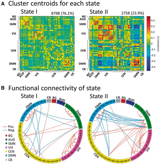
Results of the clustering analysis per state. (A) Cluster centroids for each state. The total number of occurrences and percentage of total occurrences are listed above each cluster median. (B) Only 5% of the functional connectivity matrix in each state is shown, representing the strongest connections (i.e. the largest absolute value correlation coefficients). Each square colour represents one of the seven networks. Red lines represent positive functional connectivity, and blue lines represent negative functional connectivity. BG = basal ganglia; AUD = auditory; SMN = sensorimotor; VIS = visual; CEN = cognitive executive; CB = cerebellar network.
Figure 2B shows functionally connected regions with >5% strength in each state. In State I, connections between independent components were located mainly within networks with positive correlations. In contrast, State II was characterized by connections between functional connectivity networks with positive and negative couplings.
Temporal properties of functional connectivity states in the Parkinson’s disease and healthy control groups
Figure 3A and B shows group-specific cluster centroids retrieved by the k-means clustering analysis. As noted above, in State I of healthy controls and Parkinson’s disease patients, sparse connections between independent components were located mainly within networks (sensorimotor network, visual network, and DMN) with positive coupling, whereas stronger connections between functional connectivity networks were seen mainly in State II. These included both negative coupling between the sensorimotor network and DMN (and between DMN and cognitive executive network), and positive correlations between the sensorimotor network, cognitive executive network, and visual network networks. We found a significant group difference in fractional windows (P < 0.05, Mann-Whitney U-test), which suggests that Parkinson’s disease exhibited an abnormal proportion of time spent in each state compared to healthy controls (Fig. 4A). In healthy controls, the total occurrences of State I were again more frequently observed (83.38 ± 22.28%) than State II (16.62 ± 22.28%). In the Parkinson’s disease group, however, State I occurred less frequently (70.76 ± 4.65%), and State II re-occurred at a higher rate (29.24 ± 4.65%). Thus, the compelling finding was that, in Parkinson’s disease patients, State I occurrence dropped by 12.62%, while State II presentation increased proportionally by the same amount (12.62%).
![Functional connectivity state results. (A) Group-specific cluster centroid for each state, averaged across subject-specific median cluster centroids of each group [percentage of total occurrences for stage I and II: 83.4% and 16.6% in the healthy controls (HC) and 70.8% and 29.2% in the Parkinson’s disease (PD) group, respectively]. (B) Functional connectivity in each state is shown for healthy controls and Parkinson’s disease groups, representing the 5% of the functional connectivity network with the strongest connections. BG = basal ganglia; AUD = auditory; SMN = sensorimotor; VIS = visual; CEN = cognitive executive; CB = cerebellar network.](https://oup.silverchair-cdn.com/oup/backfile/Content_public/Journal/brain/140/11/10.1093_brain_awx233/4/m_awx233f3.jpeg?Expires=1749729819&Signature=aWZO~Y8HgD3BVXq838YZULanLAaIT0K4IPpNOnueUZDDgEzeSzt4Ckre7oztMs8Kks3pXmsGtfKNz1~yeSeot1Nd2tVXF0RDzH-InWswesDOb1hpVVOiXEeHiD7b0ALHo~AZMEcLJgppWj0UdswuGDtJb0-p3dQxY7izQOF3HmXvURQoWDq~Jy00iFt~zXfm2Pv4LCtmcZLK11hwdBK-D6uVzYgPdLD6RTXlyDq4AJ8pMb6EHCBRqt7DLf5~SoTI1YvkEzluHCzOObd7WH6k5C77Oe1Ljrhta3ykLpWKrq9tkq1xlR3S9VxkwSJq8bWGucvuDjrTdSd3so~fVbQsuw__&Key-Pair-Id=APKAIE5G5CRDK6RD3PGA)
Functional connectivity state results. (A) Group-specific cluster centroid for each state, averaged across subject-specific median cluster centroids of each group [percentage of total occurrences for stage I and II: 83.4% and 16.6% in the healthy controls (HC) and 70.8% and 29.2% in the Parkinson’s disease (PD) group, respectively]. (B) Functional connectivity in each state is shown for healthy controls and Parkinson’s disease groups, representing the 5% of the functional connectivity network with the strongest connections. BG = basal ganglia; AUD = auditory; SMN = sensorimotor; VIS = visual; CEN = cognitive executive; CB = cerebellar network.

Temporal properties of functional connectivity state analysis. (A) The mean fractional windows of total subjects spent in each state as measured by percentage (i.e. total time spent in State I versus State II), (B) mean dwell time (i.e. number of consecutive windows spent in each state before switching) and (C) number of transitions (i.e. switching between states) is depicted for the Parkinson’s disease (PD) and healthy controls (HC) with error bars. Asterisks indicate a significant group difference (P < 0.05, FDR corrected).
As shown in Fig. 4B, significant group differences were identified in the mean dwell time of each state. Specifically, the mean dwell time in State I was significantly shorter in the Parkinson’s disease group compared to the healthy control group (mean ± SD for healthy controls: 115.7 ± 81.3; for Parkinson’s disease: 71.8 ± 60.8, P < 0.05, Mann-Whitney U-test, FDR corrected), implying a shorter dwell time pattern of the state with weaker connectivity. In contrast, the mean dwell time in State II was significantly longer in the Parkinson’s disease group compared to the healthy control group (healthy controls: 12.2 ± 14.3; Parkinson’s disease: 24.3 ± 20.6, P < 0.05, Mann-Whitney U-test, FDR corrected), suggesting a longer dwell time pattern of the state with stronger interconnectivity. No group differences were found with respect to the number of transitions between states (healthy controls: 3.5 ± 3.0; Parkinson’s disease: 4.2 ± 2.7, t(52) = 0.18, P = 0.38, two-sample t-test). Overall, these changes suggested that in Parkinson’s disease patients the stability of the weaker within-network functional connectivity (State I) was significantly affected, while the expression of the stronger between-network functional connectivity (State II) was instead proportionally increased.
Relationship with clinical properties
In a further analysis of correlations between dynamic functional connectivity properties and clinical characteristics in the Parkinson’s disease group, we found that dwell time in State I was negatively correlated with UPDRS-III motor symptom score (Fig. 5A; Spearman’s rho = −0.487, P < 0.05, FDR corrected), possibly indicating an association between the worsening of motor function and shortened length of stay in State I (i.e. impaired within-network functional connectivity). Additionally, the number of transitions between states was positively correlated with the UPDRS motor symptom score (Fig. 5B; Spearman’s rho = 0.518, P < 0.05, FDR corrected), suggesting a relationship between changes in dynamic states and Parkinson’s disease motor symptom severity.
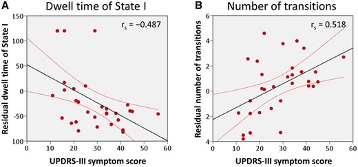
Correlation of UPDRS-III motor symptom score with temporal properties in dynamic functional connectivity for the Parkinson’s disease group. (A) The mean dwell time of State I was negatively correlated with the UPDRS-III motor symptom score, while (B) the number of state transitions was positively associated with the UPDRS-III motor symptom score in the subjects with Parkinson’s disease (all P < 0.05, FDR corrected).
Dynamic graph theory properties: network efficiency
Variance of graph metrics in time-varying brain connectivity was calculated per subject and compared between groups. Figure 6 shows the mean and bootstrapped 95% confidence intervals as well as box plots and smoothed density histograms for the variance of the local efficiency and global efficiency in each group. In general, the Parkinson’s disease group exhibited higher variance in global efficiency compared to the healthy controls group (P < 0.05, Wilcoxon rank-sum test), suggesting that the average parallel information transfer in the functional networks was less efficient, more unstable, and variable in Parkinson’s disease. In contrast, the local efficiency, measuring the average efficiency between critical nodes within a neighbourhood, was less affected (P = 0.08, Wilcoxon rank-sum test). Supplementary Fig. 4 shows graph metrics (i.e. local efficiency and global efficiency) in terms of dynamic changes across windows in all subjects.
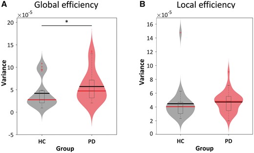
Variance of topological metrics in dynamic functional connectivity. The variances of (A) global and (B) local efficiency across the functional connectivity matrices are shown using violin plots for the healthy controls (HC) group (grey) and Parkinson’s disease (PD) group (red). Horizontal lines indicate group means (black) and medians (red). Asterisks represent significant differences at P < 0.05.
Discussion
It has been indicated that dynamic functional connectivity may reflect aspects of neural system functional capacity (Deco et al., 2011; Kucyi et al., 2017) and thus, may serve as a novel physiological biomarker of disease (Hutchison et al., 2013; Damaraju et al., 2014). The present work is the first study to investigate the dynamic functional connectivity in Parkinson’s disease patients with a focus on the temporal properties of functional connectivity states as well as variability of network topological organization. The dynamic functional connectivity analyses suggested two discrete connectivity configurations, a more frequent and sparsely connected state (State I) and a less frequent and stronger interconnected state (State II). The compelling finding was that, in Parkinson’s disease patients, the occurrence of the sparsely connected state (State I) dropped by 12.62%, while the expression of the more strongly interconnected State II increased by approximately the same amount. This is consistent with the altered temporal properties of the dynamic functional connectivity in Parkinson’s disease characterized by a shortening of dwell time of the within-network State I, paralleled by a proportional increase in the dwell time pattern of stronger interconnected State II.
Taken together, these observations seem to confirm the vulnerability of resting state networks in neurodegenerative conditions (Seeley et al., 2009; Zhou et al., 2012). It is conceptually accepted that neurodegeneration may represent a spectrum, including both ageing and disease, with overlapping neurophysiological changes. In healthy ageing, there is consistent evidence of weaker within-network functional connectivity, paralleled by a relative increase of between-network functional connectivity, interpreted as a reduced segregation of neural networks (Chan et al., 2014; Elman et al., 2016). Consistent with these reports, our observations closely resemble the trend seen in ageing and are highly suggestive of overlapping but probably more accentuated changes in Parkinson’s disease. This reduction in functional segregation was closely associated with disease expression, since the temporal dynamics of functional connectivity were closely linked to the clinical severity of Parkinson’s disease patients. In fact, worsening of motor symptoms correlated both with shortening of the dwell time of within-network State I and the increase in number of transitions between states. This explains the higher variability in network global efficiency observed in these patients, implying a less efficient and more unstable information transfer within/between functional networks and suggesting an abnormal global integration of the brain networks in Parkinson’s disease.
The observed increased expression of between-network functional connectivity showed some resemblance to the excessive neural synchronization across distributed cortical areas (described in the beta band oscillatory activity) (Laufs et al., 2003; Mantini et al., 2007), reported to be associated with motor impairment in Parkinson’s disease (Brown, 2003; Silberstein et al., 2005; Stoffers et al., 2008; Hammerer and Eppinger, 2012).
As noted above, State I was characterized by positive couplings located mainly within distinct networks (i.e. sensorimotor network, DMN and visual network), and are known to play a critical role in the pathogenesis of Parkinson’s disease symptoms. Several studies of Parkinson’s disease have identified abnormal functional connectivity in the sensorimotor network indicative of impaired sensorimotor integration (Lewis and Byblow, 2002; Tessitore et al., 2014). Visual function is also a major complex sensory domain affected by Parkinson’s disease (Mosimann et al., 2004; Weil et al., 2016). It is associated with the aberrant processing of visual information and poor visual processing sometimes leading to visual hallucinations (Cho et al., 2017). Visual-sensorimotor interaction is important for movement control and motor learning (Glickstein, 2000), which is known to be deficient in Parkinson’s disease patients (Inzelberg et al., 2008). Taken together, these results suggest that the visuomotor deficits observed in Parkinson’s disease patients may be related to the observed altered dynamic functional connectivity of the visual and sensorimotor regions. The functioning and modulation of activity within the DMN is also vital and closely anti-related with key interacting functional networks for coordinating motor and cognitive functions (Greicius et al., 2003; Fox and Raichle, 2007). The disruption of dopaminergic pathways, along with α-synuclein deposition, impacts the modulation between the DMN activity and other neural networks resulting in poor motor and cognitive performance (Christopher et al., 2015).
State II was instead characterized mainly by stronger positive couplings between networks (i.e. sensorimotor network and cognitive executive network, visual network), as well as anti-related correlations between sensorimotor network and DMN (and between DMN and cognitive executive network). The increased expression frequency of these functional couplings in our Parkinson’s disease patients, as a result of the reduced functional segregation reported beforehand, could be interpreted as a potential compensatory mechanism of intrinsic brain networks resulting in stronger synchrony. Thus, communication between central executive and sensory/motor regions (while inactivating the DMN) is required for the translation of effective cognitive processing to action (Christopher et al., 2015).
There are a few limitations that should be considered in the interpretation of our results. First, we should acknowledge the well-established effects of dopaminergic medications on resting state data, which has been examined by the strength of functional connectivity (Tahmasian et al., 2015), spectral frequency (Esposito et al., 2013), and network topology (Berman et al., 2016) measured by resting state functional MRI. For example, dopamine medication tends to normalize the strength of functional connectivity disrupted network topology in Parkinson’s disease, thereby reducing the significance of the observations (Berman et al., 2016). Although we did not find any relationship between temporal properties of dynamic functional connectivity and the levodopa equivalent daily dose in the Parkinson’s disease group, we cannot exclude the long-term effects of parkinsonian medications on our resting state data. Thus, the significance of our findings might be mitigated by the effects of dopaminergic medication. In future studies, it would be important to dissociate Parkinson’s disease-related abnormality from medication-related effects on dynamic functional connectivity properties by comparing ON and OFF conditions and with drug-naïve patients. Second, the parameter of MRI acquisition should be mentioned when it comes to dynamic functional connectivity. Fine temporal resolution and a sufficient length of acquisition are both important factors for reliable results. Previous studies (Liao et al., 2014; Allen et al., 2017) done with similar parameters as the ones used in the current study (2 TR) have reliably shown that the dynamics of fluctuation (i.e. low-frequency) can be successfully sampled with the typical repetition times we used. However, to increase the estimation power of functional connectivity matrices calculated within small windows in the sliding window approach, it would be beneficial to use a fast MRI acquisition, such as simultaneous multi-slice acquisition (Moeller et al., 2010), that could sample more dense time series. Finally, the heterogeneity of patients with Parkinson’s disease should also be considered (Eggers et al., 2012; Zhang et al., 2015b). Previous reports indicate that there may be significant differences in functional connectivity between Parkinson’s disease subtypes identified on the basis of motor symptoms (i.e. akinetic-rigid syndrome versus tremor) (Karunanayaka et al., 2016). Therefore, studies with larger sample sizes should account for differences in dynamic functional connectivity across various Parkinson’s disease subtypes.
In summary, abnormal temporal patterns and functional segregation coupled with the motor severity and higher variability of topological properties with abnormal global integration in brain networks provide new insights into the role of dynamic functional connectivity networks in Parkinson’s disease.
Funding
This work was supported by the Canadian Institutes of Health Research (MOP-136778) to A.P.S. A.P.S is supported by the Canada Research Chair Program.
Supplementary material
Supplementary material is available at Brain online.
Abbreviations
References
Author notes
See Nieuwhof and Helmich (doi:) for a scientific commentary on this article.

