 Statistical Physics of Spin Glasses and Information Processing: An Introduction
Contents
-
-
-
-
-
-
-
-
5.1 Error-correcting codes 5.1 Error-correcting codes
-
5.1.1 Transmission of information 5.1.1 Transmission of information
-
5.1.2 Similarity to spin glasses 5.1.2 Similarity to spin glasses
-
5.1.3 Shannon bound 5.1.3 Shannon bound
-
5.1.4 Finite-temperature decoding 5.1.4 Finite-temperature decoding
-
-
5.2 Spin glass representation 5.2 Spin glass representation
-
5.2.1 Conditional probability 5.2.1 Conditional probability
-
5.2.2 Bayes formula 5.2.2 Bayes formula
-
5.2.3 MAP and MPM 5.2.3 MAP and MPM
-
5.2.4 Gaussian channel 5.2.4 Gaussian channel
-
-
5.3 Overlap 5.3 Overlap
-
5.3.1 Measure of decoding performance 5.3.1 Measure of decoding performance
-
5.3.2 Upper bound on the overlap 5.3.2 Upper bound on the overlap
-
-
5.4 Infinite-range model 5.4 Infinite-range model
-
5.4.1 Infinite-range model 5.4.1 Infinite-range model
-
5.4.2 Replica calculations 5.4.2 Replica calculations
-
5.4.3 Replica-symmetric solution 5.4.3 Replica-symmetric solution
-
5.4.4 Overlap 5.4.4 Overlap
-
-
5.5 Replica symmetry breaking 5.5 Replica symmetry breaking
-
5.5.1 First-step Rsb 5.5.1 First-step Rsb
-
5.5.2 Random energy model 5.5.2 Random energy model
-
5.5.3 Replica solution in the limit r → ∞ 5.5.3 Replica solution in the limit r → ∞
-
5.5.4 Solution for finite r 5.5.4 Solution for finite r
-
-
5.6 Codes with finite connectivity 5.6 Codes with finite connectivity
-
5.6.1 Sourlas-type code with finite connectivity 5.6.1 Sourlas-type code with finite connectivity
-
5.6.2 Low-density parity-check code 5.6.2 Low-density parity-check code
-
5.6.3 Cryptography 5.6.3 Cryptography
-
-
5.7 Convolutional code 5.7 Convolutional code
-
5.7.1 Definition and examples 5.7.1 Definition and examples
-
5.7.2 Generating polynomials 5.7.2 Generating polynomials
-
5.7.3 Recursive convolutional code 5.7.3 Recursive convolutional code
-
-
5.8 Turbo code 5.8 Turbo code
-
5.9 CDMA multiuser demodulator 5.9 CDMA multiuser demodulator
-
5.9.1 Basic idea of Cdma 5.9.1 Basic idea of Cdma
-
5.9.2 Conventional and Bayesian demodulators 5.9.2 Conventional and Bayesian demodulators
-
5.9.3 Replica analysis of the Bayesian demodulator 5.9.3 Replica analysis of the Bayesian demodulator
-
5.9.4 Performance comparison 5.9.4 Performance comparison
-
-
Bibliographical note Bibliographical note
-
-
-
-
-
-
-
Cite
Abstract
Reliable transmission of information through noisy channels plays a vital role in modern society. Some aspects of this problem have close formal similarities to the theory of spin glasses. Noise in the transmission channel can be related to random interactions in spin glasses and the bit sequence representing information corresponds to the Ising spin configuration. The replica method serves as a powerful tool of analysis, and TAP-like equations can be used as a practical implementation of the algorithm to infer the original message. The gauge theory also provides an interesting point of view. This chapter introduces these problems.
Reliable transmission of information through noisy channels plays a vital role in modern society. Some aspects of this problem have close formal similarities to the theory of spin glasses. Noise in the transmission channel can be related to random interactions in spin glasses and the bit sequence representing information corresponds to the Ising spin configuration. The replica method serves as a powerful tool of analysis, and TAP-like equations can be used as a practical implementation of the algorithm to infer the original message. The gauge theory also provides an interesting point of view.
5.1 Error-correcting codes
Information theory was initiated by Shannon half a century ago. It formulates various basic notions on information transmission through noisy channels and develops a framework to manipulate those abstract objects. We first briefly review some ideas of information theory, and then restate the basic concepts, such as noise, communication, and information inference, in terms of statistical mechanics of spin glasses.
5.1.1 Transmission of information
Suppose that we wish to transmit a message (information) represented as a sequence of N bits from one place to another. The path for information transmission is called a (transmission) channel. A channel usually carries noise and the output from a channel is different in some bits from the input. We then ask ourselves how we can infer the original message from the noisy output.
It would be difficult to infer which bit of the output is corrupted by noise if the original message itself had been fed into the channel. It is necessary to make the message redundant before transmission by adding extra pieces of information, by use of which the noise can be removed. This process is called channel coding (or encoding), or simply coding. The encoded message is transmitted through a noisy channel. The process of information retrieval from the noisy output of a channel using redundancy is called decoding.
A very simple example of encoding is to repeat the same bit sequence several (for instance, three) times. If the three sequences received at the end of the channel coincide, one may infer that there was no noise. If a specific bit has different values in the three sequences, one may infer its correct value (0 or 1) by the majority rule. For example, when the original message is (0, 0, 1, 1, 0) and the three output sequences from a noisy channel are (0, 0, 1, 1, 0), (0, 1, 1, 1, 0), and (0, 0, 1, 1, 0), the correct second bit can be inferred to be 0 whereas all the other bits coincide to be (0, *, 1, 1, 0). This example shows that the redundancy is helpful to infer the original information from the noisy message.
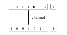
A more sophisticated method is the parity-check code. For example, suppose that seven bits are grouped together and one counts the number of ones in the group. If the number is even, one adds 0 as the eighth bit (the parity bit) and adds 1 otherwise. Then there are always an even number of ones in the group of eight bits in the encoded message (code word). If the noise rate of the channel is not very large and at most only one bit is flipped by noise out of the eight received bits, one may infer that the output of the channel carries no noise when one finds even ones in the group of eight bits. If there are odd ones, then there should be some noise, implying error detection (Fig. 5.1). Error correction after error detection needs some further trick to be elucidated in the following sections.
5.1.2 Similarity to spin glasses
It is convenient to use the Ising spin ±1 instead of 0 and 1 to treat the present problem by statistical mechanics. The basic operation on a bit sequence is the sum with modulo 2 (2=0 with mod 2), which corresponds to the product of Ising spins if one identifies 0 with S i = 1 and 1 with S i = −1. For example, 0 + 1 = 1 translates into 1 × (−1) = −1 and 1 + 1 = 0 into (−1) x (−1) = 1. We hereafter use this identification of an Ising spin configuration with a bit sequence.
Generation of the parity bit in the parity-check code corresponds to the product of appropriate spins. By identifying such a product with the interaction between the relevant spins, we obtain a spin system very similar to the Mattis model of spin glasses.
In the Mattis model one allocates a randomly quenched Ising spin ξ i to each site, and the interaction between sites i and j is chosen to be J ij = ξiξj. The Hamiltonian is then

The ground state is clearly identical to the configuration of the quenched spins S i = ξ i (∀i) (or its total reversal S i = —ξ i (∀i)), see Fig. 5.2(a).
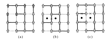
The ground-state spin configurations of the Mattis model without noise added (a), the interaction marked by a cross flipped by noise (b), and three interactions flipped by strong noise (c). Thin lines represent ferromagnetic interactions and bold lines antiferromagnetic interactions. The plaquettes marked by dots are frustrated.
Returning to the problem of error-correcting codes, we form the Mattis-type interactions
For instance, the conventional r = 2 Mattis model on the two-dimensional square lattice has NB = 2N interactions, the number of neighbouring sites. Forthe original interactions without noise J0 ={ξiξj}, the product of the
5.1.3 Shannon bound
It is necessary to introduce redundancy appropriately to transmit information accurately through a noisy channel. It can indeed be proved that such redundancy should exceed a threshold so that we are able to retrieve the original message without errors.
Let us define the transmission rate R of information by a channel as

For smaller denominator, the redundancy is smaller and the transmission rate is larger. Strictly speaking, the numerator of (5.2) should be the 'number of informative bits in the original message'. For biased messages, where 0 and 1 appear with unequal probabilities, the amount of information measured in bits is smaller than the length of the binary message itself. This can easily be verified by the extreme case of a perfectly biased message with only ones; the message carries no information in such a case. By multiplying (5.2) by the number of bits transmitted per second, one obtains the number of information bits transmitted per second.
We consider a memoryless binary symmetric channel (BSC) where noise flips a bit from 1 to 0 and 0 to 1 independently at each bit with a given probability. It is known that the transmission rate should satisfy the following inequality so that error-free transmission is possible through the BSC in the limit of a very long bit sequence:

where C is a function of the noise probability and is called the channel capacity. The capacity of the BSC is

Here p is the probability that a bit is flipped by noise. Equation (5.3) is called the channel coding theorem of Shannon and implies that error-free transmission is possible if the transmission rate does not exceed the channel capacity and an appropriate procedure of encoding and decoding is employed. Similar results hold for other types of channels such as the Gaussian channel to be introduced later. A sketch of the arguments leading to the channel coding theorem is given in Appendix C.
An explicit example of a code that saturates the Shannon bound (5.3) asymptotically as an equality is the Sourlas code (Sourlas 1989): one takes all possible products of r spins from N sites to form Mattis-type interactions. We have mainly explained the conventional Mattis model with r = 2 in §5.1.2, and we discuss the general case of an arbitrary r (= 2, 3, 4, …) hereafter. This is nothing but the infinite-range model with r-body interactions.5 It will be shown later that the Shannon bound (5.3) is asymptotically achieved and the error rate approaches zero in the Sourlas code if we take the limit N → ∞ first and r → ∞ afterwards. It should be noted, however, that the inequality (5.3) reduces to an equality with both sides approaching zero in the Sourlas code, which means that the transmission rate R is zero asymptotically. Therefore the transmission is not very efficient. A trick to improve this point was shown recently to be to take the product of a limited number of combinations, not all possible combinations of r spins, from N sites. All of these points will be elucidated in detail later in the present chapter.
5.1.4 Finite-temperature decoding
Let us return to the argument of §5.1.2 and consider the problem of inference of spin configurations when the noise probability is not necessarily small. It was shown in §5.1.2 that the ground state of the Ising spin system (with the output of the channel as interactions) is the true original message (spin configuration) if the channel is not very noisy. For larger noise, the ground state is different from the original spin configuration (Fig. 5.2(c)). This suggests that the original spin configuration is one of the excited states and thus one may be able to decode more accurately by searching for states at finite temperature. It will indeed be shown that states at a specific finite temperature T p determined by the error rate p give better results under a certain criterion. This temperature T p turns out to coincide with the temperature at the Nishimori line discussed in Chapter 4 (Ruján 1993).
5.2 Spin glass representation
We now formulate the arguments in the previous section in a more quantitative form and proceed to explicit calculations (Sourlas 1989).
5.2.1 Conditional probability
Suppose that the Ising spin configuration ξ= {ξi} has been generated according to a probability distribution function P(ξ). This distribution P(ξ) for generating the original message is termed the prior. Our goal is to infer the original spin configuration from the output of a noisy channel as accurately as possible. Following the suggestion in the previous section, we form a set of products of r spins

for appropriately chosen combinations of the ξi and feed the set of interactions into the channel. We first consider the BSC, and the output of the channel

where βp is a function of p defined as

Equation (5.6) is equal to 1 − p when
Assume that (5.6) applies to each set (i l … i r) independently. This is a memoryless channel in which each bit is affected by noise independently. The overall probability is then the product of (5.6)

where the sum in the exponent is taken over all sets (i l … i r) for which the spin products are generated by (5.5). The symbol NB is for the number of terms in this sum and is equal to the number of bits fed into the channel.
5.2.2 Bayes formula
The task is to infer the original message (spin configuration) ξ from the output J = {
The joint probability P(A,B) that two events A and B occur is expressed in terms of the product of P(B) and the conditional probability P(A|B) for A under the condition that B occurred. The same holds if A and B are exchanged. Thus we have

It follows immediately that

Equation (5.10) is the Bayes formula.
We can express P(σ|J) in terms of (5.8) using the Bayes formula:

We have written σ = {σ1, …, σN} for dynamical variables used for decoding. The final decoded result will be denoted by
The probability P(J|σ) represents the characteristics of a memoryless BSC and is given in (5.8). It is therefore possible to infer the original message by (5.11) if the prior P(σ) is known. Explicit theoretical analysis is facilitated by assuming a message source that generates various messages with equal probability. This assumption is not necessarily unnatural in realistic situations where information compression before encoding usually generates a rather uniform distribution of zeros and ones. In such a case, p(σ) can be considered a constant. The posterior is then

Since J is given and fixed in the present problem, (5.12) is nothing more than the Boltzmann factor of an Ising spin glass with randomly quenched interactions J. We have thus established a formal equivalence between the probabilistic inference problem of messages for a memoryless BSC and the statistical mechanics of the Ising spin glass.
5.2.3 MAP and MPM
Equation (5.12) is the probability distribution of the inferred spin configuration σ, given the output of the channel J. Then the spin configuration to maximize (5.12) is a good candidate for the decoded (inferred) spin configuration. Maximization of the Boltzmann factor is equivalent to the ground-state search of the corresponding Hamiltonian

This method of decoding is called the maximum a posteriori probability (MAP). This is the idea already explained in §5.1.2. Maximization of the conditional probability P(J|σ) with respect to σ is equivalent to maximization of the posterior P(σ|J) if the prior P(σ) is uniform. The former idea is termed the maximum likelihood method as P(J|σ) is the likelihood function of σ.
The MAP maximizes the posterior of the whole bit sequence σ. There is another strategy of decoding in which we focus our attention on a single bit i, not the whole sequence. This means we trace out all the spin variables except for a single σi to obtain the posterior only of σi. This process is called marginalization in statistics:

We then compare P(σ i = 1|J) and p(σi = — 1|J) and, if the former is larger, we assign one to the decoded result of the ith bit
It is instructive to consider the MPM from a different point of view. The MPM is equivalent to accepting the sign of the difference of two probabilities as the ith decoded bit

This may also be written as

5.2.4 Gaussian channel
It is sometimes convenient to consider channels other than the BSC. A typical example is a Gaussian channel. The encoded message

If the prior is uniform, the posterior is written using the Bayes formula as

Comparison of this equation with (5.12) shows that the posterior of the Gaussian channel corresponds to that of the BSC with β p replaced by J 0/J 2. We can therefore develop the following arguments for both of these channels almost in the same way.
5.3 Overlap
5.3.1 Measure of decoding performance
It is convenient to introduce a measure of success of decoding that represents the proximity of the decoded message to the original one. The decoded ith bit is
The product of

which is the overlap of the original and decoded messages. We have denoted the sum over the site variables ξ by Trξ and the one over the bond variables J by

This expression may be regarded as the average of sgn <σi>β with the weight proportional to Z(βp)
The overlap is closely related with the Hamming distance of the two messages (the number of different bits at the corresponding positions). For closer messages, the overlap is larger and the Hamming distance is smaller. When the two messages coincide, the overlap is one and the Hamming distance is zero, while, for two messages completely inverted from each other, the overlap is −1 and the Hamming distance is N.
5.3.2 Upper bound on the overlap
An interesting feature of the overlap M(β) is that it is a non-monotonic function of β with its maximum at β = β p:

In other words the MPM at the correct parameter value β = β P gives the optimal result in the sense of maximization of the overlap (Ruján 1993; Nishimori 1993; Sourlas 1994; Iba 1999). The MPM is sometimes called the Bayes-optimal strategy.
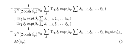
To prove (5.21), we first take the absolute value of both sides of (5.20) and exchange the absolute value operation and the sum over J to obtain

where we have used |sgn<σi>β| = 1. By rewriting the right hand side as follows, we can derive (5.21):

Almost the same manipulations lead to the following inequality for the Gaussian channel:

We have shown that the bit-wise overlap defined in (5.19) is maximized by the MPM with the correct parameter (β = β p for the BSC). This is natural in that the MPM at β = β P was introduced to maximize the bit-wise (marginalized) posterior. The MAP maximizes the posterior of the whole bit sequence σ, but its probability of error for a given single bit is larger than the MPM with the correct parameter value. This observation is also confirmed from the viewpoint of Bayesian statistics (Sourlas 1994; Iba 1999).
The inequalities (5.21) and (5.24) are essentially identical to (4.63) derived by the gauge theory in §4.6.4. To understand this, we note that generality is not lost by the assumption ξi = 1(∀i) in the calculation of M(β) for a uniform information source. This may be called the ferromagnetic gauge. Indeed, the gauge transformation
5.4 Infinite-range model
Inequality (5.21) shows that M(β) is a non-monotonic function, but the inequality does not give the explicit β-dependence. It may also happen that it is not easy to adjust β exactly to β P in practical situations where one may not know the noise rate p very precisely. One is then forced to estimate β p but should always be careful of errors in the parameter estimation. It is therefore useful if one can estimate the effects of errors in the parameter estimation on the overlap M(β).
A solvable model, for which we can calculate the explicit form of M(β), would thus be helpful as a guide for non-solvable cases. The infinite-range model serves as an important prototype for this and other purposes.
5.4.1 Infinite-range model
The Sourlas code explained in §5.1.3 is represented as the infinite-range model. In the Sourlas code, the sum in the Hamiltonian

runs over all possible combinations of r spins out of N spins. Then the number of terms is
The parameters J 0 and J in the Gaussian distribution (5.17) must be scaled appropriately with N so that the expectation value of the infinite-range Hamiltonian (5.25) is extensive (proportional to N) in the limit N → ∞. If we also demand that physical quantities remain finite in the limit r → ∞ after N → ∞, then r should also be appropriately scaled. The Gaussian distribution satisfying these requirements is

where J and j 0 are independent of N and r. The appropriateness of (5.26) is justified by the expressions of various quantities to be derived below that have non-trivial limits as N → ∞ and r → ∞.
5.4.2 Replica calculations
Following the general prescription of the replica method, we first calculate the configurational average of the nth power of the partition function and take the limit n → 0. Order parameters naturally emerge in due course. The overlap M is expressed as a function of these order parameters.
The configurational average of the nth power of the partition function of the infinite-range model is written for the uniform prior (P = 2−N) as
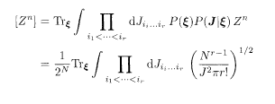

where α (= 1, …, n) is the replica index. A gauge transformation

in (5.27) removes ξ from the integrand. The problem is thus equivalent to the case of ξ i = 1(∀i) the ferromagnetic gauge. We mainly use this gauge in the present chapter. The sum over ξin (5.27) then simply gives 2n, and the factor 2−N in front of the whole expression disappears.
It is straightforward to carry out the Gaussian integral in (5.27). If we ignore the trivial overall constant and terms of lower order in N, the result is
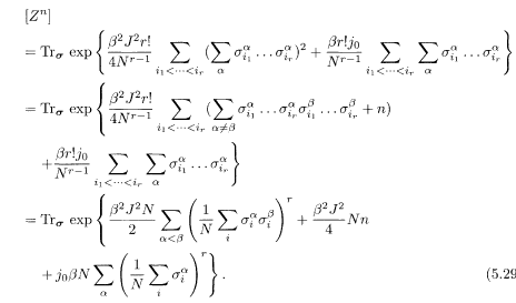
Here Trσ is the sum over σ. In deriving the final expression, we have used a relation that generalizes the following relation to the r-body case:

It is convenient to introduce the variables

to replace the expressions inside the parentheses in the final expression of (5.29) by q αβ and m α so that we can carry out the Trσ. operation. The condition to satisfy (5.31) is imposed by the Fourier-transformed expressions of delta functions with integration variables
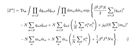
We can now operate Trσ independently at each i to find
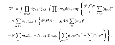
Here Tr denotes sums over single-site replica spins {σ 1, …, σ n}.
5.4.3 Replica-symmetric solution
Further calculations are possible under the assumption of replica symmetry:

We fix n and take the thermodynamic limit N → ∞ to evaluate the integral by steepest descent. The result is

where

The equations of state for the order parameters are determined by the saddlepoint condition. By variation of (5.36), we obtain


where

These reduce to the equations of state for the conventional SK model, (2.28) and (2.30), when r = 2. One should remember that 2j 0 here corresponds to J 0 in the conventional notation of the SK model as is verified from (5.27) with r = 2.
5.4.4 Overlap
The next task is to derive the expression of the overlap M. An argument similar to §2.2.5 leads to formulae expressing the physical meaning of q and m:

Comparison of (5.41) and (5.39) suggests that tanh2 β(.) and tanh β(.) in the integrands of the latter may be closely related with <σ i>2 and <σ i> in the former. To confirm this, we add
It should now be clear that the additional external field with the product of k spins,

Thus, for an arbitrary function F(x) that can be expanded around x = 0, the following identity holds:

The overlap is, in the ferromagnetic gauge, M(β) = [sgn<σ i>β]. If we therefore take as F(x) a function that approaches sgn(x) (e.g. tanh(ax) with a → ∞), we obtain the desired relation for the overlap:

It has thus been established that M(β) is determined as a function of q and m through G.
5.5 Replica symmetry breaking
The system (5.25) and (5.26) in the ferromagnetic gauge is a spin glass model with r-body interactions. It is natural to go further to investigate the properties of the RSB solution (Derrida 1981; Gross and Mèzard 1984; Gardner 1985; Nishimori and Wong 1999; Gillin et al. 2001). We shall show that, for small values of the centre of distribution j 0, a 1RSB phase appears after the RS paramagnetic phase as the temperature is lowered. A full RSB phase follows at still lower temperature. For larger j 0, paramagnetic phase, ferromagnetic phase without RSB, and then ferromagnetic phase with RSB phases appear sequentially as the temperature is decreased.
5.5.1 First-step Rsb
The free energy with 1RSB can be derived following the method described in §3.2

where x (0 ≤ x ≤ 1) is the boundary of q o and q 1 in the matrix block, denoted by m 1 in §3.2. Extremization of (5.45) with respect to

Elimination of


These equations coincide with (3.32)−(3.34) for r = 2 if we set h = 0 and 2j o = J 0. The equation of extremization by x does not have an intuitively appealing compact form so that we omit it here.
The AT stability condition of the RS solution is

The criterion of stability for 1RSB is expressed similarly. For the replica pair (αβ) in the same diagonal block, the stability condition for small deviations of q αβ and

Further steps of RSB take place with the diagonal blocks breaking up into smaller diagonal and off-diagonal blocks. Thus it is sufficient to check the intra-block stability condition (5.52) only.
5.5.2 Random energy model
The model in the limit r → ∞ is known as the random energy model (REM) (Derrida 1981). The problem can be solved completely in this limit and the spin glass phase is characterized by 1RSB.
As its name suggests, the REM has an independent distribution of energy. Let us demonstrate this fact for the case of j 0 = 0. The probability that the system has energy E will be denoted by P(E),

The average [• • •] over the distribution of J, (5.26), can be carried out if we express the delta function by Fourier transformation. The result is

The simultaneous distribution function of the energy values E 1 and E 2 of two independent spin configurations σ (1) and σ (2) with the same set of interactions can be derived similarly:

It is easy to see in the limit r → ∞ that

which implies independence of the energy distributions of two spin configurations. Similar arguments hold for three (and more) energy values.
The number of states with energy E is, according to the independence of energy levels,

This expression shows that there are very many energy levels for

We then have, from dS/dE = 1/T,

The free energy is therefore

where
5.5.3 Replica solution in the limit r → ∞
It is instructive to rederive the results of the previous subsection by the replica method. We first discuss the case j 0 = 0. It is quite reasonable to expect no RSB in the paramagnetic (P) phase at high temperature. We thus set

This agrees with (5.60) for T > T c.
It is necessary to introduce RSB in the spin glass (SG) phase. We try 1RSB and confirm that the result agrees with that of the previous subsection. For the 1RSB to be non-trivial (i.e. different from the RS), it is required that q 0 < q 1 ≤ 1 and

Variation with respect to x gives

The highest temperature satisfying this equation is the following one for x = 1:

and therefore, for T <TC,

This agrees with (5.60), which confirms that 1RSB is exact in the temperature range T < T ϲ. It is also possible to show by explicit k-step RSB calculations that the solution reduces to the 1RSB for any k (≥1) (Gross and Mèzard 1984).
It is easy to confirm that x < 1 for T < T ϲ from (5.63); generally, x = T/T ϲ. The order parameter function q(x) is equal to 1 (= q 1) above x (= T/T ϲ) and 0 (= q 0) below x (see Fig. 5.3).
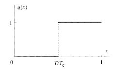
Spin glass order parameter of the REM below the transition temperature
For j 0 exceeding some critical value, a ferromagnetic (F) phase exists. It is easy to confirm that the solution of (5.48), (5.49), and (5.47) in the limit r → ∞ is q 0 = q x = m = 1 when j0 > 0, m > 0. The ferromagnetic phase is therefore replica symmetric since q 0 = q 1. The free energy (5.36) is then

The phase boundaries between these three phases are obtained by comparison of the free energies:
P–SG transition:
SG-F transition:
P–F transition:
The final phase diagram is depicted in Fig. 5.4.
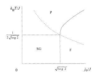
Phase diagram of the REM. The Nishimori line is shown dashed.
Let us now turn to the interpretation of the above results in terms of error-correcting codes. The overlap M is one in the ferromagnetic phase

As shown in Appendix C, the capacity of the Gaussian channel is

Here we substitute

The transmission rate (5.67), on the other hand, reduces in the same limit to

It has thus been established that the transmission rate R coincides with the channel capacity C at the lower limit of the ferromagnetic phase
The general inequality (5.21) is of course satisfied. Both sides vanish if j 0 < (j 0)c- For j 0 > (j 0)c, the right hand side is one while the left hand side is zero in the paramagnetic phase and one in the ferromagnetic phase. In other words, the Sourlas code in the limit r → ∞ makes it possible to transmit information without errors under the MAP as well as under the MPM. An important point is that the information transmission rate R is vanishingly small, impeding practical usefulness of this code.
The Nishimori line βJ 2 = J 0 is in the present case T/J = J/(2j 0) and passes through the point at
5.5.4 Solution for finite r
It is necessary to solve the equations of state numerically for general finite r.7 The result for the case of r = 3 is shown here as an example (Nishimori and Wong 1999; Gillin et al. 2001). If jo is close to zero, one finds a 1RSB SG solution with q 1 > 0 and q 0 = m = 0 below T = 0.651 J. As the temperature is lowered, the stability condition of the 1RSB (5.52) breaks down at T = 0.240J, and the full RSB takes over.
The ferromagnetic phase is RS (5.39) in the high-temperature range but the RSB should be taken into account below the AT line (3.22); a mixed (M) phase with both ferromagnetic order and RSB exists at low temperatures. The ferromagnetic phase, with RS and/or RSB, continues to exist beyond the limit of thermodynamic stability as a metastable state (i.e. as a local minimum of the free energy). Figure 5.5 summarizes the result.
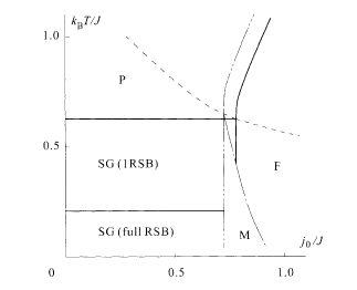
Phase diagram of the model with r = 3. The double dotted line indicates the limit of metastability (spinodal) of the ferromagnetic phase. Error correction is possible to the right of this boundary. Thermodynamic phase boundaries are drawn in full lines. The Nishimori line is drawn dashed.
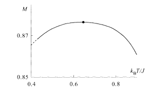
Dependence of the overlap M(β) on T (= 1/β) is depicted in Fig. 5.6 where j 0/J is fixed to 0.77 close to the boundary of the ferromagnetic phase. The overlap M(β) is a maximum at the optimal temperature T/J = J/2j 0 = 0.649 appearing on the right hand side of (5.24) corresponding to the Nishimori line (the dot in Fig. 5.6). The ferromagnetic phase disappears above T/J= 0.95 even as a metastable state and one has M = 0: the paramagnetic phase has <σ i>β =0 at each site i, and sgn <σ i>β cannot be defined. It is impossible to decode the message there. For temperatures below T/J = 0.43, the RSB is observed (the dashed part). We have thus clarified in this example how much the decoded message agrees with the original one as the temperature is changed around the optimal value.
5.6 Codes with finite connectivity
The Sourlas code saturates the Shannon bound asymptotically with vanishing transmission rate. A mean-field model with finite connectivity has a more desirable property that the rate is finite yet the Shannon bound is achieved. We state some of the important results about this model in the present section. We refer the reader to the original papers cited in the text for details of the calculations.
5.6.1 Sourlas-type code with finite connectivity
The starting point is analogous to the Sourlas code described by the Hamiltonian (5.25) but with diluted binary interactions for the BSC,

where the element of the symmetric tensor

The code rate is R = r/c because an encoded message has c bits per index i and carries r bits of the original information.
Using the methods developed for diluted spin glasses (Wong and Sherrington 1988), one can calculate the free energy under the RS ansatz as (Kabashima and Saad 1998, 1999; Vicente et al. 1999)

Here [• • •] J and [•••]ξ denote the configurational averages over the distributions of J and ξ, respectively. The order functions π(x) and

where a and â are normalization constants, and l is the number of replica indices on the left hand side. Extremization of the free energy gives paramagnetic and ferromagnetic solutions for the order functions. The spin glass solution should be treated with more care under the 1RSB scheme. The result becomes relatively simple in the limit where r and c tend to infinity with the ratio R = r/c(= l/α) kept finite and F = 0:

where p is the noise probability of the BSC, and

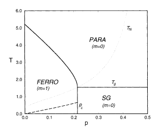
Finite-temperature phase diagram of the unbiased diluted Sourlas code with R= 1/4 in the limit r, c → ∞ (Vicente et al. 1999). The Shannon bound is achieved at p c. The ferromagnetic phase is stable at least above the dashed line. (Copyright 1999 by the American Physical Society)
The ferromagnetic solution appears as a metastable state at a very high temperature of O(r/log r), but the thermodynamic transition takes place at T of O(1). This suggests that there exists a high energy barrier between the ferromagnetic and paramagnetic solutions. Consequently, it might be difficult to reach the correctly decoded (i.e. ferromagnetic) state starting from an arbitrary initial condition (which is almost surely a paramagnetic state) by some decoding algorithm. We are therefore lead to consider moderate r, in which case the ferromagnetic phase would have a larger basin of attraction although we have to sacrifice the final quality of the decoded result (magnetization smaller than unity). In Fig. 5.8 the ground-state magnetization (overlap) is shown as a function of the noise probability for various finite values of r (written as K in the figure) in the case of R = 1/2. The transition is of first order except for r = 2. It can be seen that the decoded result is very good (m close to one) for moderate values of r and p.
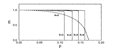
Ground-state magnetization as a function of the noise probability for various r (written as K in the figure) (Vicente et al 1999). The rate R is 1/2 and F = 0. Also shown by open circles are the numerical results from the TAP-like decoding algorithm. (Copyright 1999 by the American Physical Society)
It is useful to devise a practical algorithm of decoding, given the channel output {Jμ}, where μ denotes an appropriate combination of site indices. The following method based on an iterative solution of TAP-like equations is a powerful tool for this purpose (Kabashima and Saad 2001; Saad et al. 2001) since its computational requirement is only of O(N). For a given site i and an interaction μ that includes i, one considers a set of conditional probabilities

where ν also includes i.8 Under an approximate mean-field-like decoupling of the conditional probabilities, one obtains the following set of equations for m μi and

where M(i) is a set of interactions that include i, and L (μ) is a set of sites connected by J μ. After iteratively solving these equations for m μi and

This method is equivalent to the technique of belief propagation used in information theory. It is also called a TAP approach in the statistical mechanics literature owing to its similarity to the TAP equations in the sense that m μi and
The resulting numerical data are shown in Fig. 5.8. One can see satisfactory agreement with the replica solution. It also turns out that the basin of attraction of the ferromagnetic solution is very large for r = 2 but not for r ≥ 3.
5.6.2 Low-density parity-check code
Statistical-mechanical analysis is applicable also to other codes that are actively investigated from the viewpoint of information theory. We explain the low-density parity-check code (LDPC) here because of its formal similarity to the diluted Sourlas code treated in the previous subsection (Kabashima et al. 2000a; Murayama et al. 2000). In statistical mechanics terms, the LDPC is a diluted many-body Mattis model in an external field.9
Let us start the argument with the definition of the code in terms of a Boolean representation (0 and 1, instead of ±1). The original message of length N is denoted by an N-dimensional Boolean vector ξ and the encoded message of length M by z 0. The latter is generated from the former using two sparse matrices C s and C n according to the following modulo-2 operation of Boolean numbers:

The matrix C s has the size M × N and the number of ones per row and column randomly. The channel noise ζ is added to z 0, and the output is

Decoding is carried out by multiplying z by C n:

One finds the most probable solution of this equation for the decoded message σ and the inferred noise τ

The Ising spin representation corresponding to the above prescription of the LDPC, in particular (5.83), is

where L s(μ) is a set of indices of non-zero elements in the μth row of C s and similarly for L n(μ). Note that σ, τ, ξ, and ζ are all Ising variables (±1) from now on. The Hamiltonian reflects the constraint (5.84) as well as the bias in the original message and the channel noise:

Here A is a sparse tensor for choosing the appropriate combination of indices corresponding to C s and C n (or L s(μ) and L s(μ)), F s is the bias of the original message, and F n =
The replica analysis of the present system works similarly to the diluted Sourlas code. The resulting RS free energy at T = 0 is


The order functions π(x) and

Extremization of the free energy (5.86) with respect to these order functions yields ferromagnetic and paramagnetic solutions. Since the interactions in the Hamiltonian (5.85) are of Mattis type without frustration, there is no spin glass phase. When r ≥ 3 or l ≥ 3, r > 1, the free energy for an unbiased message (F s = 0) is

The spin alignment is perfect (m = 1) in the ferromagnetic phase. The magnetization as a function of the channel-error probability p is shown in Fig. 5.9(a). The ferromagnetic state has a lower free energy below p c that coincides with the Shannon bound as can be verified by equating f F and f P. The paramagnetic solution loses its significance below p c because its entropy is negative in this region. A serious drawback is that the basin of attraction of the ferromagnetic state is quite small in the present case.
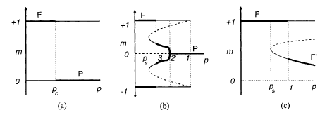
Magnetization as a function of the channel-error probability in the LDPC (Murayama et al 2000). Bold lines represent stable states, (a) r ≥ 3 or l ≥ 3, r > 1. (b) r = l = 2. (c) r = 1. (Copyright 2000 by the American Physical Society)
If r = l = 2, the magnetization behaves as in Fig. 5.9(b). The perfect ferromagnetic state and its reversal are the only solutions below a threshold p s. Any initial state converges to this perfect state under an appropriate decoding algorithm. Thus the code with r = l = 2 is quite useful practically although the threshold p s lies below the Shannon bound.
The system with single-body interactions r = 1 has the magnetization as shown in Fig. 5.9(c). Again, the Shannon bound is not saturated, but the perfect ferromagnetic state is the only solution below p s. An advantage of the present case is that there is no mirror image (m = −1).
Iterative solutions using TAP-like equations work also in the LDPC as a rapidly converging tool for decoding (Kabashima and Saad 2001; Saad et al. 2001). These equations have similar forms to (5.78) but with two types of parameters, one for the σ-spins and the other for τ. Iterative numerical solutions of these equations for given dilute matrices C s and C n show excellent agreement with the replica predictions.
5.6.3 Cryptography
The LDPC is also useful in public-key cryptography (Kabashima et al. 20006). The N-dimensional Boolean plaintext ξ is encrypted to an M-dimensional ciphertext z by the public key

Only the authorized user has the knowledge of C n, C s, and D separately, not just the product G. The authorized user then carries out the process of decryption equivalent to the decoding of the LDPC to infer D ξ and consequently the original plaintext ξ. This user succeeds if r = l = 2 and p < p s as was discussed in the previous subsection.
The task of decomposing G into C n, C s, and D is NP complete10 and is very difficult for an unauthorized user, who is therefore forced to find the ground state of the Hamiltonian, which is the Ising spin representation of (5.89):

where G is a dense tensor with elements 1 or 0 corresponding to G, and ϑ is either 1 or – 1 according to the noise added as ζ in the Boolean representation (5.89). Thus the system is frustrated. For large N, the number r' in the above Hamiltonian and c' (the connectivity of the system described by (5.90)) tend to infinity (but are smaller than N itself) with the ratio c'/r' kept finite. The problem is thus equivalent to the Sourlas-type code in the same limit. We know, as mentioned in §5.6.1, that the basin of attraction of the correctly decrypted state in such a system is very narrow. Therefore the unauthorized user almost surely fails to decrypt.
This system of cryptography has the advantage that it allows for relatively high values of p, and thus an increased tolerance against noise in comparison with existing systems. The computational requirement for decryption is of O(N), which is much better than some of the commonly used methods.
5.7 Convolutional code
The convolutional code corresponds to a one-dimensional spin glass and plays important roles in practical applications. It also has direct relevance to the turbo code, to be elucidated in the next section, which is rapidly becoming the standard in practical scenes owing to its high capability of error correction. We explain the convolutional code and its decoding from a statistical-mechanical point of view following Montanari and Sourlas (2000).
5.7.1 Definition and examples
In a convolutional code, one first transforms the original message sequence ξ = {ξ 1,….ξ N}(ξ i = ±1,∀i)into a register sequence τ = {τ 1(ξ),…,τ N(ξ)} (τ i = ±1, ∀i). In the non-recursive convolutional code, the register sequence coincides with the message sequence (τ i = ξ i, ∀i) but this is not the case in the recursive convolutional code to be explained later in §5.7.3. To encode the message, one prepares r registers, the state of which at time t is described by

The encoder thus carries the information of (r + 1) bits τ t, τ t – 1, …, τ t – r at any moment t.
We restrict ourselves to the convolutional code with rate R = 1/2 for simplicity. Code words

Here, α = 1 or 2, and we define τ j = 1 for j ≤ 0. The superscript k(j; α) is either 0 or 1 and characterizes a specific code. We define k(0; 1) = k(0; 2) = 1 to remove ambiguities in code construction. Two simple examples will be used frequently to illustrate the idea:
k(0; 1) = k(1;1) = 1, and the other k(j; 1) = 0; k(0; 2) = 1, and the other k(j; 2) = 0. The memory order is r = 1. The code words are

where
k(0; 1) = k(1; 1) = k(2; 1) = 1, and the other k(j; 1) = 0; k(0; 2) = k(2; 2) = 1, and the other k(j; 2) = 0. The memory order is r = 2 and the code words are

which can be regarded as a system of ladder-like structures shown in Fig. 5.10. A diagrammatic representation of the encoder is depicted in Fig. 5.11.
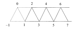
A convolutional code with code rate 1/2 (example 2 in the text) expressed as a spin system. Interactions exist among three spins around each triangle and between two horizontally neighbouring spins. Two up spins are located at i = – 1 and i = 0 to fix the initial condition.
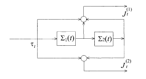
Encoder corresponding to the code of Fig. 5.10.
5.7.2 Generating polynomials
Exposition of the encoding procedure in terms of the Boolean (0 or 1) representation instead of the binary (±1) representation is useful to introduce the recursive convolutional code in the next subsection. For this purpose, we express the original message sequence ξ ={ξ1,….ξN} by its generating polynomial defined as

where H j(= 0 or 1) is the Boolean form of ξj: ξj =

The non-recursive convolutional code has G(x) = H(x), but this is not the case for the recursive code to be explained in the next subsection. The code word J (α)(α = 1,2) is written as

with

as

or equivalently

The right hand side is the convolution of k and G, from which the name of convolutional code comes.
The examples 1 and 2 of §5.7.1 have the generating polynomials as
5.7.3 Recursive convolutional code
The relation between the source and register sequences ξ and τ (or H (x) and G(x)) is not simple in the recursive convolutional code. The register sequence of recursive convolutional code is defined by the generating polynomial as

Code words satisfy

The first relation means J (1) = ξ in the binary representation.
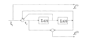
Encoder of the recursive convolutional code to be compared with the non-recursive case of Fig. 5.11.
The relation between the source and register sequences (5.101) can be written in terms of the binary representation as follows. Equation (5.101) is seen to be equivalent to

This equation allows us to determine τ i recursively; that is, is determined if we know τ 1….,τ i–1. From the definition

The encoder for the code of example 2 of §5.7.1 is shown in Fig. 5.12. Decoding is carried out under the Hamiltonian

where

which is to be contrasted with the non-recursive case

5.8 Turbo code
The turbo code is a powerful coding/decoding technique frequently used recently. In has near-optimal performance (i.e. the transmission rate can be made close to the Shannon bound under the error-free condition), which is. exceptional in a practicable code. We explain its statistical-mechanical formulation and some of the results (Montanari and Sourlas 2000; Montanari 2000).
The turbo code is a variant of the recursive convolutional code with the source message sequence ξ={ξ 1,…ξ N} the permuted sequence ξ P = {ξ P(1), … ξ P(N)}as the input to the encoder. The permutation P operates on the set {1, 2, …, N} and is fixed arbitrarily for the moment. Correspondingly, two register sequences are generated according to the prescription of the recursive convolutional code (5.103):


or, equivalently,


The code words are comprised of three sequences and the rate is R= 1/3:

The posterior to be used at the receiving end of the channel has the following expression:


where the Hamiltonian is, corresponding to (5.112),

The interactions

The finite-temperature (MPM) decoding with the appropriate β is used in practice because an efficient TAP-like finite-temperature iterative algorithm exists as explained later briefly.
To understand the effectiveness of turbo code intuitively, it is instructive to express the spin variable
The decoding algorithm of the turbo code is described as follows. One prepares two chains labelled by α = 1, 2 with the Hamiltonian

Then one iteratively solves a set of TAP-like equations for the effective fields


where <…>(α) is the thermal average with the Hamiltonian H (α) (σ (α)) and k denotes the iteration step. The process (5.116)−(5.118) is an approximation to the full system (5.114) and yet yields excellent performance numerically.
Detailed statistical-mechanical analysis of the system H (1)(σ (1)) + H (2)(σ (2)) with ε P(i)(σ (1)) = ε i(σ (2)) has been carried out (Montanari 2000). We describe some of its important results. Let us suppose that the channel is Gaussian and (3 is adjusted to the optimal value (MPM). The S/N ratio is denoted as 1/w 2. There exists a phase of error-free decoding (overlap M = 1) that is locally unstable in the high-noise region

The limit of the first example (w c = 0.721) is found to be close to numerical results whereas the second (w c = 1.675) shows some deviation from numerical results. The stability analysis leading to these values may not give the correct answer if a first-order phase transition takes place in the second example.
5.9 CDMA multiuser demodulator
In this section we present a statistical-mechanical analysis of signal transmission by modulation (T. Tanaka 2001). This topic deviates somewhat from the other parts of this chapter. The signal is not encoded and decoded but is modulated and demodulated as described below. Nevertheless, the goal is very similar to error-correcting codes: to extract the best possible information from a noisy output using the idea of Bayesian inference.
5.9.1 Basic idea of Cdma
Code-division multiple access (CDMA) is an important standard of modern mobile communications (Simon et al. 1994; Viterbi 1995). The digital signal of a user is modulated and transmitted to a base station through a channel that is shared by multiple users. At the base station, the original digital signal is retrieved by demodulation of the received signal composed of the superposition of multiple original signals and noise. An important problem is therefore to design an efficient method to modulate and demodulate signals.
In CDMA, one modulates a signal in the following way. Let us focus our attention to a signal interval which is the time interval carrying a single digital signal, with a signal ξ i (= ±1) for the ith user. The signal interval is divided into p chip intervals (p = 4 in Fig. 5.13). User i is assigned a spreading code sequence

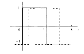
Modulation of the signal of a single user in CDMA. A signal interval is composed of four chip intervals in this example. The full line represents the original signal and the dashed line denotes the spreading code sequence.
at the chip interval t and is asked to retrieve the original signals ξ i (i = 1, …, N) from y t(t = l,…,p) with the knowledge of the spreading code sequence
Before proceeding to the problem of demodulation, we list a few points of idealization that lead to the simple formula (5.120): modulated signals of N users are assumed to be transmitted under perfect synchronization at each chip interval t throughout an information signal interval. This allows us simply to sum up
The measure of performance is the overlap of the original (ξ i) and demodulated

averaged over the distributions of
5.9.2 Conventional and Bayesian demodulators
Let us first explain the simple method of the conventional demodulator. To extract the information of ξ i from y t, we multiply the received signal at the tth chip interval y t by the spreading code

The first term on the right hand side is the original signal, the second represents multiuser interference, and the third is the channel noise (which is assumed to be Gaussian). We then demodulate the signal by taking the sign of this quantity

It is easy to analyse the performance of this conventional demodulator in the limit of large N and p with α = p/N fixed. We also assume that the noise power

where Erf(x) is the error function
To improve the performance, it is useful to construct the posterior of the original signal, given the noisy signal, following the method of Bayesian inference. Let us denote the set of original signals by ξ= t{ξ 1,….ξ N} and the corresponding dynamical variables for demodulation by S = t(S 1,…, SN) The sequence of received signals within p chip intervals is also written as a vector in a p-dimensional space y = t(y 1,…, y p). Once the posterior p(S\y) is given, one demodulates the signal by the MAP or MPM:


To construct the posterior, we first write the distribution of Gaussian noise

where the effective Hamiltonian has been defined as

The field hi has already been defined in (5.122). If we assume that the prior is uniform, P(ξ) = const, the posterior is seen to be directly proportional to the prior according to the Bayes formula:

The Hamiltonian (5.128) looks very similar to the Hopfield model to be discussed in Chapter 7, (7.7) with (7.4), the only difference being that the sign of the interaction is the opposite (Miyajima et al. 1993).
5.9.3 Replica analysis of the Bayesian demodulator
The replica method is useful to analyse the performance of the Bayesian demodulator represented by the posterior (5.129).
Since we usually do not know the noise power of the channel βs, it is appropriate to write the normalized posterior with an arbitrary noise parameter β in place of βs, the latter being the true value. From (5.127)−(5.129), we then find

where the vector r denotes t(r 1,…, r p) with

The factor 2−N is the uniform prior for ξ. The macroscopic behaviour of the system is determined by the free energy averaged over the distributions of the spreading code sequence, which is assumed to be completely random, and the channel noise. The latter distribution of noise is nothing more than the partition function (5.131) with the true hyperparameter β = βs, which we denote by Zo(r). The replica average is therefore expressed as

where the configurational average on the right hand side is over the spreading code sequence. It is convenient to separate the above quantity into the spin-dependent part g 1 and the rest g 2 for further calculations:

where α = p/N in the exponent should not be confused with the replica index. The zeroth replica (α= 0) corresponds to the probability weight Z 0. The two functions g 1 and g 2 are defined by


where the following notations have been used:

In the thermodynamic limit p,N → ∞ with their ratio α fixed, these v 0 and v α become Gaussian variables with vanishing mean and covariance given by the overlap of spin variables, under the assumption of a random distribution of the spreading code sequence:

To proceed further, we assume symmetry between replicas (α = l,…,n): Q0α=m, Q0αβ=q(α,β≥1). Then v 0 and v α are more conveniently written in terms of independent Gaussian variables u, t, and z α with vanishing mean and unit variance,

We are now ready to evaluate the factor
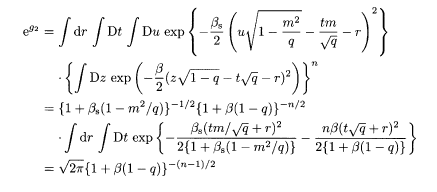

The other factor


where we have used the RS form of the matrix M 0α = E and M αβ = F (α≠ β ≥ 1). In the thermodynamic limit, the leading contribution is


Extremization of the free energy yields the equations of state for the order parameters as


The overlap is determined from these quantities by

The stability limit of the RS solution, the AT line, is expressed as

The optimum demodulation by MPM is achieved at the parameter β = βs whereas the MAP corresponds to β → ∞.
5.9.4 Performance comparison
The results of the previous analysis in terms of the bit-error rate (1 − M)/2 are plotted in Fig. 5.14 for (a) βs = 1 and (b) βs = 20 for the conventional demodulator (CD), MPM ('Opt.'), and MAP demodulators. Also shown is the mean-field demodulator in which one uses the mean-field equation of state for local magnetization

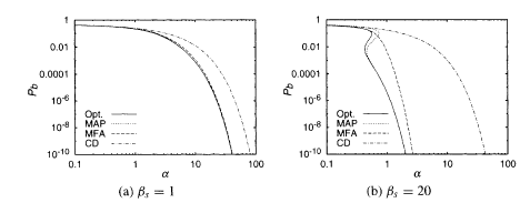
Bit-error rate of the CDMA demodulators. The left one (a) is for the noise power βs = 1 and the right (b) is for βs = 20. The symbols are: Opt. for the MPM, MFA for the mean-field demodulator with β = βs , and CD for the conventional demodulator (T. Tanaka 2001; Copyright 2001 by the Massachusetts Institute of Technology).
in combination with
It is observed that the MAP and MPM show much better performance than the conventional demodulator. The curve for the MAP almost overlaps with the MPM curve when the noise power is high, βs = 1, but a clear deviation is found in the low-noise case βs = 20. The MPM result has been confirmed to be stable for RSB. By contrast, one should take RSB into account for the MAP except in a region with small α and large βs.
Bibliographical note
General expositions of information theory and error-correcting codes are found in textbooks on these subjects (McEliece 1977; Clark and Cain 1981; Lin and Costello 1983; Arazi 1988; Rhee 1989; Ash 1990; Wicker 1995). The present form of statistical-mechanical analysis of error-correcting codes was proposed by Sourlas (1989) and has been expanding rapidly as described in the text. Some of the recent papers along this line of development (but not cited in the text) include Kanter and Saad (2000), Nakamura et al. (2000), and Kabashima et al. (2000 c). See also Heegard and Wicker (1999) for the turbo code.
The symbol p is often used in the literature to denote the number of interacting spins. We use r instead to avoid confusion with the error probability in the BSC.
Remember that we are using the ferromagnetic gauge.
The original source message is assumed to be generated sequentially from i = 1 to i = N. Consequently the time step denoted by t (= 1, 2, …,N) is identified with the bit number i(= 1,2,…, N).
| Month: | Total Views: |
|---|---|
| October 2022 | 5 |
| November 2022 | 4 |
| December 2022 | 4 |
| March 2023 | 3 |
| April 2023 | 2 |
| May 2023 | 2 |
| July 2023 | 4 |
| September 2023 | 6 |
| October 2023 | 2 |
| December 2023 | 7 |
| January 2024 | 16 |
| February 2024 | 3 |
| March 2024 | 21 |
| April 2024 | 3 |
| May 2024 | 5 |
| June 2024 | 7 |
| July 2024 | 10 |
| August 2024 | 1 |
| October 2024 | 4 |
| November 2024 | 4 |
| December 2024 | 5 |
| January 2025 | 7 |
| February 2025 | 5 |
| March 2025 | 3 |
| April 2025 | 11 |
| May 2025 | 9 |