


Summary
In this study, a longitudinal regression model for covariance matrix outcomes is introduced. The proposal considers a multilevel generalized linear model for regressing covariance matrices on (time-varying) predictors. This model simultaneously identifies covariate-associated components from covariance matrices, estimates regression coefficients, and captures the within-subject variation in the covariance matrices. Optimal estimators are proposed for both low-dimensional and high-dimensional cases by maximizing the (approximated) hierarchical-likelihood function. These estimators are proved to be asymptotically consistent, where the proposed covariance matrix estimator is the most efficient under the low-dimensional case and achieves the uniformly minimum quadratic loss among all linear combinations of the identity matrix and the sample covariance matrix under the high-dimensional case. Through extensive simulation studies, the proposed approach achieves good performance in identifying the covariate-related components and estimating the model parameters. Applying to a longitudinal resting-state functional magnetic resonance imaging data set from the Alzheimer’s Disease (AD) Neuroimaging Initiative, the proposed approach identifies brain networks that demonstrate the difference between males and females at different disease stages. The findings are in line with existing knowledge of AD and the method improves the statistical power over the analysis of cross-sectional data.
1. Introduction
In neuroimaging studies, understanding functional changes in and between healthy and pathological brains is an essential topic. With repeated measurements, longitudinal analysis enables the assessment of within-individual changes as well as the articulation of systematic differences among individuals. One representative example is neurodegenerative studies. With demographic shifts in aging, Alzheimer’s disease (AD) and related dementias are a major public health challenge. Understanding disease pathology, identifying biological markers, and suggesting early diagnosis and intervention strategies are critically important. The landmark Alzheimer’s Disease Neuroimaging Initiative (ADNI) study aims to identify biomarkers for the early detection and tracking of AD to assist in the development of prevention and intervention strategies. In the study, longitudinal data were collected from various measurement domains, including clinical, genetic, imaging, and biospecimen, after obtaining informed consent. Motivated by this longitudinal resting-state fMRI data set, we propose to extend Model (1.1) to appropriately integrate information collected at multiple visits to increase the statistical power of identifying covariate-related effects.
A classic way of analyzing longitudinal neuroimaging data is to extract voxel/regional data first and subsequently fit them with a univariate longitudinal analysis model, such as a hierarchical or mixed-effects model or generalized estimating equations, one at a time, and then finish with a multiple testing correction procedure (see a review by Madhyastha and others, 2018). In fMRI studies, the study interest lies more in the exploration of the interactions between voxels/regions or the network-level properties (Li and others, 2009; Dai and others, 2017). Univariate approaches disregard network information and structured constraints in the data. For resting-state fMRI data, the covariance matrix of the signals is generally used to reveal the coactivation between units, so-called functional connectivity (Friston, 2011). Running longitudinal models on an individual element of the matrix ignores the positive definiteness resulting in a large number of hypothesis testing. Thus, it is deficient in statistical power and prevents the ability to predict a valid functional connectivity matrix. Multivariate approaches, including principal component analysis (PCA) and independent component analysis (ICA), are generally applied for dimension reduction. However, investigations of longitudinal effects on brain networks are rare. Recently, a hierarchical ICA model was proposed to analyze longitudinal fMRI data enabling the study of time-dependent effects on the IC decomposition (Wang and Guo, 2019). Graph theory is a technique widely used in resting-state fMRI studies to reveal the topological architecture of brain networks. With longitudinal data, it offers a way of studying the temporal variations in the topological structures (Madhyastha and others, 2018). However, the method can be sensitive to the definition of the graphs. For example, under different choices of brain parcellation or due to the statistical variation in graph estimation, the findings can be highly heterogeneous (Farahani and others, 2019). For the purpose of predicting a behavioral outcome, machine learning techniques, such as support vector machines, random forests, and neural networks, together with cross-validation are widely implemented. However, these approaches usually ignore the temporal dependency in the repeated measures. Thus, they cannot be used to reveal the within-subject variation and track longitudinal changes (Telzer and others, 2018).
In this study, the focus is on identifying covariate-related brain networks in a longitudinal setting. It is assumed that the linear projection, |${\boldsymbol{\gamma}}$|, in (1.1) is a constant over time. A multilevel model is proposed to capture the within-subject variation in the covariance matrix. Under normality assumptions, a likelihood-based approach is introduced to estimate the parameters. For the case with high-dimensional data, by generalizing the proposal in Zhao and others (2021a), a linear shrinkage estimator of the covariance matrices is introduced. The shrinkage parameter is assumed to be common across subjects and visits. By doing so, the estimator achieves the uniformly minimum quadratic loss asymptotically among all linear combinations of the identity matrix and the sample covariance matrix.
The rest of the article is organized as the following. Section 2 introduces the longitudinal regression model for covariance matrix outcomes. The estimation method is proposed, and the asymptotic properties are studied. In Section 3, the performance of the proposed approach is demonstrated through simulation studies. In Section 4, the model is applied to a longitudinal resting-state fMRI data set collected by the ADNI study. Section 5 summarizes this manuscript with discussions. The technical proofs and additional simulation and analytical results are collected in the Supplementary material available at Biostatistics online.
2. Model and methods
No structural assumption on the covariance matrices is imposed. Rather, it is assumed that there exists at least one common linear projection that satisfies (2.2). For the case of high dimensionality, to yield a consistent estimate of the covariance matrix, structural assumptions, such as bandable covariance matrices, sparse covariance matrices, spiked covariance matrices, covariances with a tensor product structure, and latent graphical models, are generally imposed in many regularization-based methods (Cai and others, 2016). In the next section, a shrinkage estimator of the covariance matrices is introduced, which does not require any structural assumption. In addition, the estimator is guaranteed to be positive definite, preserves the eigenstructure of the covariance matrices, and is easy to compute based on a simple and explicit formula.
2.1. Methods
For the case of high-dimensional data, |$\max_{i,v}T_{iv}\ll p$| with |$p$| increasing to infinity, the sample covariance matrices are rank deficient. The estimate of the eigenvalues and eigenvectors can be largely biased (Bickel and Levina, 2008) and optimizing (2.4) is numerically unstable. Generalizing the shrinkage estimator proposed in Zhao and others (2021a) to a longitudinal setting, the solution to the following optimization problem is considered as an estimate of the covariance matrices.
It is assumed that the shrinkage parameters, |$\rho$| and |$\mu$|, are constant over visits and subjects. One can also assume constant shrinkage parameters over visits for each subject. As demonstrated in Theorem A.5 in Section A.2 of the Supplementary material available at Biostatistics online, the empirical solution to (2.5) gives the optimal estimator that yields the uniformly minimum quadratic loss asymptotically among all linear combinations of the identity matrix and the sample covariance matrix.
Denote |${\mathbf{w}}_{iv}=(1,{\mathbf{x}}_{1i}^\top,{\mathbf{x}}_{2iv}^\top)^\top\in\mathbb{R}^{q+1}$| and |${\boldsymbol{\beta}}_{i}=(\beta_{0i},{\boldsymbol{\beta}}_{1}^\top,{\boldsymbol{\beta}}_{2i}^\top)^\top\in\mathbb{R}^{q+1}$|, and, |$\beta_{0i}+{\mathbf{x}}_{1i}^\top{\boldsymbol{\beta}}_{1}+{\mathbf{x}}_{2iv}^\top{\boldsymbol{\beta}}_{2i}={\mathbf{w}}_{iv}^\top{\boldsymbol{\beta}}_{i}$|. The following theorem gives the solution to the optimization problem.
For |$\forall~v\in\{1,\dots,V_{i}\}$| and |$\forall~i\in\{1,\dots,n\}$|, |$\delta_{iv}^{2}=\phi_{iv}^{2}+\psi_{iv}^{2}$|, and thus, |$\delta^{2}=\phi^{2}+\psi^{2}$|.
2.2. Algorithm
The optimization algorithm for problems (2.4) and (2.5).
Input:|$\{({\mathbf{y}}_{iv1},\dots,{\mathbf{y}}_{ivT_{iv}}),{\mathbf{x}}_{iv}~|~v=1,\dots,V_{i},~i=1,\dots,n\}$|
- 1:
initialization: |$({\boldsymbol{\gamma}}^{(0)},\beta_{0i}^{(0)},{\boldsymbol{\beta}}_{1}^{(0)},{\boldsymbol{\beta}}_{2i}^{(0)},\beta_{0}^{(0)},\sigma^{2(0)},{\boldsymbol{\beta}}_{2}^{(0)},{\boldsymbol{\Omega}}^{(0)})$|
- 2:
repeat for iteration |$s=0,1,2,\dots$|
- 3:|$\; \; \; \;$|for |$v=1,\dots,V_{i}$| and |$i=1,\dots,n$|, update$$ {\mathbf{S}}_{iv}^{*(s+1)}=\frac{\hat{\psi}^{2(s)}}{\hat{\delta}^{2(s)}}\mu^{(s)}\boldsymbol{\mathrm{I}}+\frac{\hat{\phi}^{2(s)}}{\hat{\delta}^{2(s)}}{\mathbf{S}}_{iv}, $$
|$\; \; \; \;$| where |$(\hat{\psi}^{2},\hat{\phi}^{2},\hat{\delta}^{2},\mu)$| are set to the value with |${\boldsymbol{\gamma}}={\boldsymbol{\gamma}}^{(s)}$|, |$\beta_{0i}=\beta_{0i}^{(s)}$|, |${\boldsymbol{\beta}}_{1}={\boldsymbol{\beta}}_{1}^{(s)}$|, and |${\boldsymbol{\beta}}_{2i}={\boldsymbol{\beta}}_{2i}^{(s)}$|,
- 4:
|$\; \; \; \;$|update |${\boldsymbol{\gamma}}$|, |$\beta_{0i}$|, |${\boldsymbol{\beta}}_{1}$|, |${\boldsymbol{\beta}}_{2i}$|, |$\beta_{0}$|, |$\sigma^{2}$|, |${\boldsymbol{\beta}}_{2}$|, and |${\boldsymbol{\Omega}}$| by solving (2.4) with |$\hat{\Sigma}_{iv}={\mathbf{S}}_{iv}^{*(s+1)}$|, denoted as |${\boldsymbol{\gamma}}^{(s+1)}$|, |$\beta_{0i}^{(s+1)}$|, |${\boldsymbol{\beta}}_{1}^{(s+1)}$|, |${\boldsymbol{\beta}}_{2i}^{(s+1)}$|, |$\beta_{0}^{(s+1)}$|, |$\sigma^{2(s+1)}$|, |${\boldsymbol{\beta}}_{2}^{(s+1)}$|, and |${\boldsymbol{\Omega}}^{(s+1)}$|, respectively,
- 5:
until the objective function in (2.4) converges;
- 6:
consider a random series of initializations, repeat Steps 1–5, and choose the results with the minimum objective value.
Output: |$(\hat{{\boldsymbol{\gamma}}},\hat{\beta}_{0i},\hat{{\boldsymbol{\beta}}}_{1},\hat{{\boldsymbol{\beta}}}_{2i},\hat{\beta}_{0},\hat{\sigma}^{2},\hat{{\boldsymbol{\beta}}}_{2},\hat{{\boldsymbol{\Omega}}})$|
When assuming a constant slope for those time-varying covariates, that is the variance of the corresponding |${\boldsymbol{\beta}}_{2i}$| is zero, one can combine those covariates with |${\mathbf{x}}_{i}$| in the estimation. Algorithm 1 presents a generic scenario with time-invariant and time-varying covariates. If only one type exists, appropriate modification can be made by dropping the related terms from the likelihood function.
2.3. Inference
To draw inference on the parameters, a bootstrap procedure is employed, which has been proven to yield satisfactory results with a small sample size under minimal assumptions (Van der Leeden and others, 2008). In this study, we propose a nonparametric bootstrapping procedure. Consider the case that the number of visits is small, for example, no more than five visits. We resample the subjects with replacement and keep the visit data for each subject intact (Van der Leeden and others, 2008; Goldstein, 2011). Theoretical and simulation studies show that bootstrapping on the highest level offers better performance and a more accurate reflection of the original sample information (Ren and others, 2010). Using all the samples, an estimate of |${\boldsymbol{\gamma}}$| is first obtained, denoted as |$\hat{{\boldsymbol{\gamma}}}$|. For the |$b$|th replication, the subjects are resampled with replacement. For each subject, the data from all visits and all the observations at each visit are used to estimate the model parameters, |$(\beta_{0i},{\boldsymbol{\beta}}_{1},{\boldsymbol{\beta}}_{2i},\beta_{0},\sigma^{2},{\boldsymbol{\beta}}_{2},{\boldsymbol{\Omega}})$|, by setting |${\boldsymbol{\gamma}}=\hat{{\boldsymbol{\gamma}}}$|. This procedure is repeated for |$B$| times. Confidence intervals of the coefficient parameters are then calculated using either the percentile or bias-corrected approach (Efron, 1987). Here, we focus on the inference of the model coefficient parameters. Bootstrap inference on |${\boldsymbol{\gamma}}$| requires a matching procedure of the |${\boldsymbol{\gamma}}$| estimates across different bootstrap samples, because the order of identifying the components, as well as the number of components, may differ across bootstrap samples. Meanwhile, the quality of matching and the different metrics used for matching may impact the inference. In addition, the computation cost associated with estimating |${\boldsymbol{\gamma}}$| and matching will significantly increase the total computation time. Thus, this is one of our future research directions.
2.4. Asymptotic properties
Let |$({\boldsymbol{\gamma}}^{*},\beta_{0}^{*},\sigma^{2*},{\boldsymbol{\beta}}_{1}^{*},{\boldsymbol{\beta}}_{2s}^{*},{\boldsymbol{\Omega}}^{*})$| denote the true parameters. We discuss the asymptotic properties of the proposed estimator under two scenarios: (i) |$p<\min_{i,v}T_{iv}$| and fixed and (ii) |$p>\max_{i,v}T_{iv}$|. When |$p<\min_{i,v}T_{iv}$| and fixed, one can replace |$\hat{\Sigma}_{iv}$| with the sample covariance matrix, |${\mathbf{S}}_{iv}$|, in (2.3). Minimizing (2.3) is then equivalent to maximizing the hierarchical-likelihood function. Thus, with |${\boldsymbol{\gamma}}={\boldsymbol{\gamma}}^{*}$|, the estimator of |$(\beta_{0}^{*},\sigma^{2*},{\boldsymbol{\beta}}_{1}^{*},{\boldsymbol{\beta}}_{2}^{*},{\boldsymbol{\Omega}}^{*})$| is consistent (Andersen, 1970; Lee and Nelder, 1996).
When assuming that all the covariance matrices have the same set of eigenvectors, the estimator of |${\boldsymbol{\gamma}}$| by Algorithm 1 (denoted as |$\hat{{\boldsymbol{\gamma}}}$|) is a consistent estimator based on the theory of maximum likelihood estimator. Thus, the estimator of |$(\beta_{0}^{*},\sigma^{2*},{\boldsymbol{\beta}}_{1}^{*},{\boldsymbol{\beta}}_{2}^{*},{\boldsymbol{\Omega}}^{*})$| under |$\hat{{\boldsymbol{\gamma}}}$| is also consistent.
Now, we discuss the case of |$p>\max_{i,v}T_{iv}$|. Under this scenario, one should replace |$\hat{\Sigma}_{iv}$| with the proposed shrinkage estimator rather than the sample covariance matrix as |${\mathbf{S}}_{iv}$| is rank deficient. This is a generalization of the proposal in Zhao and others (2021a) to a longitudinal setting, thus we leave all the detailed discussion, such as the imposed assumptions, to Section A.2 of the Supplementary material available at Biostatistics online and only present the main result here. Let |$\bar{{\mathbf{S}}}=\sum_{i=1}^{n}\sum_{v=1}^{V_{i}}T_{iv}{\mathbf{S}}_{iv}/\sum_{i=1}^{n}\sum_{v=1}^{V_{i}}T_{iv}$| denote the average sample covariance matrix over subjects and visits. Under Assumptions A2 and A5 of the Supplementary material available at Biostatistics online, |$\bar{{\mathbf{S}}}$| is guaranteed to be positive definite and the eigenvectors of |$\bar{{\mathbf{S}}}$| are consistent estimators (Anderson, 1963). Taking the eigenvectors of |$\bar{{\mathbf{S}}}$| as the initial values of |${\boldsymbol{\gamma}}$|, the estimators from Algorithm 1 are consistent.
Under Assumptions A1–A5 (in Section A.2 of the Supplementary material available at Biostatistics online), as |$n,T\rightarrow\infty$|, the estimator of |$({\boldsymbol{\gamma}}^{*},\beta_{0}^{*},{\boldsymbol{\beta}}_{1}^{*},{\boldsymbol{\beta}}_{2}^{*})$| obtained by Algorithm 1 is asymptotically consistent. In addition, as |$n,V,T\rightarrow\infty$|, the estimator of |$(\sigma^{2*},{\boldsymbol{\Omega}}^{*})$| is asymptotically consistent.
3. Simulation study
In this section, we present the performance of the proposed method through simulation studies. Comparisons with other competing methods under the cross-sectional setting were studied for the case of |$p<T_{\min}$| and |$p>T_{\max}$| in Zhao and others (2021c) and Zhao and others (2021a), respectively. In this article, we compare the proposed longitudinal covariate-assisted principal regression approach (denoted as LCAP) with a longitudinal approach derived from the approach in Zhao and others (2021a) (denoted as CAP-mix). The CAP-mix approach includes three steps: (i) apply the covariance regression model in Zhao and others (2021a) to the data collected at the first visit to estimate the projection and shrinkage parameters; (ii) use the estimates to acquire the log-transformed scores, |$\log(\hat{{\boldsymbol{\gamma}}}^\top\hat{\Sigma}_{iv}\hat{{\boldsymbol{\gamma}}})$|, for each subject at each visit; and (iii) fit these scores in a mixed-effects model to yield the estimate and inference of |${\boldsymbol{\beta}}$|.
In this longitudinal simulation study, for subject |$i$| at visit |$v$|, the covariance matrices are generated using the eigendecomposition |$\Sigma_{iv}=\Pi\Lambda_{iv}\Pi^\top$|, where |$\Pi=({\boldsymbol{\pi}}_{1},\dots,{\boldsymbol{\pi}}_{p})$| is an orthonormal matrix in |$\mathbb{R}^{p\times p}$| and |$\Lambda_{iv}=\mathrm{diag}\{\lambda_{iv1},\dots,\lambda_{ivp}\}$| is a diagonal matrix. A case of two covariates is considered (thus |$q=3$|), a binary outcome generated from a Bernoulli distribution with probability |$0.5$| to be one and a continuous outcome generated from a normal distribution with mean zero and variance |$0.5^2$|. The intercept coefficient, |$\beta_{0}$|, exponentially decays from |$3$| to |$-3$|, and |$\beta_{0i}$| is generated from a normal distribution with mean |$\beta_{0}$| and variance |$\sigma^{2}=0.1^{2}$|. Two dimensions, D2 and D4, are chosen to be related to the covariates. For D2, |$\beta_{1}=-0.5$| and |$\beta_{2}=0.5$|; for D4, |$\beta_{1}=0.5$| and |$\beta_{2}=-0.25$|; and for the rest, |$\beta_{1}=\beta_{2}=0$|. For both LCAP and CAP-mix methods, the number of components is chosen with |$\mathrm{DfD}(\hat{{\boldsymbol{\Gamma}}}^{(k)})< 2$|. The performance of estimating the number of components under this threshold has been studied in Zhao and others (2021c). Thus, we will not repeat here. In this article, we only present the result of identifying D4 for demonstration. For |${\boldsymbol{\beta}}$|, we choose to present the result of estimating |$\beta_{2}$| as it has a relatively smaller effect size.
We first consider a case of |$p=20$| and set |$n=50,100,500$|, |$V_{i}=V=5,50$|, and |$T_{iv}=T=50,100,500$| to examine the finite sample performance. The results are presented in Figure 1. From the figures, as |$n$| and |$T$| increase, the estimate of |$\beta$| and |${\boldsymbol{\gamma}}$| converge to the truth. For the variance of the random intercept, |$\sigma^{2}$|, as |$V$| increases, the performance improves and the estimate converges to the truth consisting with the theoretical results. We compare the performance of the proposed LCAP approach with the CAP-mix approach in the setting with a higher dimension, |$p=100$|. Table 1 presents the results. Though LCAP achieves slightly higher bias under lower sample size with |$V=5$| and |$T_{iv}=T=50$|, when either of |$V$| and |$T$| increases, the performance of LCAP improves that it yields lower bias and mean squared error (MSE) in estimating |$\beta$| and higher correlation to the truth in estimating |${\boldsymbol{\gamma}}$|. It should be noted that when |$V=5$| and |$T_{iv}=T=500$|, the LCAP approach yields superior performance in estimation bias and MSE, however, the coverage probability (CP) of |$\beta$| estimate is lower. The confidence interval (CI) of the LCAP approach is obtained from |$500$| bootstrap samples, while the CI of the CAP-mix approach is obtained from the fitted mixed-effects model in Step (3) of CAP-mix described above, which is a theoretical parametric confidence interval. Thus, a lower CP of the LCAP approach may be due to the nonparametric resampling-based inference procedure. In addition, as |$V$| increases, the performance of CAP-mix does not improve and the CP of |$\beta$| estimate decreases. Thus, for longitudinal data, the proposed LCAP approach is a more appropriate choice. In Section C.1 of the Supplementary material available at Biostatistics online, robustness under model misspecification is examined and discussed. When the linear model is misspecified, the proposed approach correctly identifies the covariate-related projection vectors while the estimate of the coefficients can be biased. Though the asymptotic consistency requires the eigenvectors to be common across subjects and visits, numerical evaluations suggest that this can be relaxed to partial common diagonalization. The findings are consistent with the results under the cross-sectional setting (Zhao and others, 2021a; Zhao and others, 2021c).
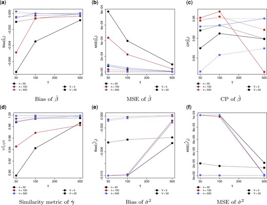
Estimation performance in estimating the parameters in the simulation study. For |$\hat{\beta}$|, (a) bias, (b) mean squared error (MSE), and (c) coverage probability (CP) from |$500$| bootstrap samples. For |$\hat{{\boldsymbol{\gamma}}}$|, (e) similarity to |${\boldsymbol{\pi}}_{j}$|. For |$\sigma^{2}$|, (e) bias and (f) MSE. Data dimension |$p=20$|. Sample sizes vary from |$n=50,100,500$|, |$V_{i}=V=5,50$|, and |$T_{iv}=T=50,100,500$|.
Bias, mean squared error (MSE), and coverage probability (CP) in estimate |$\beta$|, the similarity of |$\hat{{\boldsymbol{\gamma}}}$| to |${\boldsymbol{\pi}}_{j}$|, and the MSE in estimating the eigenvalues in the simulation study. Data dimension |$p=100$|, sample size |$n=50,$| and |$T_{iv}=T=50,500$|, and the number of visits |$V=5,50$|. For CAP-mix, the CP is calculated from the mixed-effects model; for LCAP, the CP is calculated from |$500$| bootstrap samples
| |$V$| | |$T$| | Method | |$\hat{\beta}$| | |$\hat{{\boldsymbol{\gamma}}}$| | |$\hat{\lambda}_{ij}$| | ||
|---|---|---|---|---|---|---|---|
| Bias | MSE (|$\times 10^{-3}$|) | CP | |$|\langle \hat{{\boldsymbol{\gamma}}},{\boldsymbol{\pi}}_{j} \rangle|$| (SE) | MSE | |||
| |$5$| | |$50$| | CAP-mix | |$0.006$| | |$0.749$| | |$0.950$| | |$0.842$| (|$0.043$|) | |$0.188$| |
| LCAP | |$-0.011$| | |$0.864$| | |$0.761$| | |$0.618$| (|$0.053$|) | |$0.192$| | ||
| |$500$| | CAP-mix | |$0.007$| | |$0.083$| | |$1.000$| | |$0.834$| (|$0.027$|) | |$0.162$| | |
| LCAP | |$-0.002$| | |$0.071$| | |$0.766$| | |$0.938$| (|$0.011$|) | |$0.141$| | ||
| |$50$| | |$50$| | CAP-mix | |$0.020$| | |$0.524$| | |$0.376$| | |$0.833$| (|$0.049$|) | |$0.207$| |
| LCAP | |$-0.004$| | |$0.096$| | |$0.766$| | |$0.938$| (|$0.012$|) | |$0.163$| | ||
| |$500$| | CAP-mix | |$0.008$| | |$0.078$| | |$0.235$| | |$0.846$| (|$0.025$|) | |$0.143$| | |
| LCAP | |$0.001$| | |$0.006$| | |$0.946$| | |$0.993$| (|$0.001$|) | |$0.129$| | ||
4. The Alzheimer’s Disease Neuroimaging Initiative Study
We apply the proposed approach to the magnetic resonance imaging (MRI) data collected by the Alzheimer’s Disease Neuroimaging Initiative (ADNI, adni.loni.usc.edu). The ADNI study was launched in 2003 as a public–private partnership, led by Principal Investigator Michael W. Weiner, MD. The primary goal of ADNI has been to test whether serial MRI, positron emission tomography, other biological markers, and clinical and neuropsychological assessments can be combined to measure the progression of mild cognitive impairment (MCI) and early Alzheimer’s disease (AD).
In the study, resting-state fMRI data were collected at multiple visits. In this study, we focus on the first |$V=5$| visits (initial screening, 3-month, 6-month, 1-year, and 2-year visit) for sample size consideration, where |$n=78$| subjects with at least three continuous visits are studied (|$11$| subjects with |$3$| visits, |$29$| with |$4$| visits, and |$38$| with |$5$| visits). At the initial screening, |$14$| are cognitive normal (CN) subjects (|$6$| Female), |$41$| diagnosed with MCI (|$16$| Female), and |$23$| diagnosed with AD (|$11$| Female). The fMRI time courses are extracted from |$p=75$| brain regions (|$60$| cortical and |$15$| subcortical regions), which are grouped into 10 functional modules, using the Harvard-Oxford Atlas in FSL (Smith and others, 2004). For each time course, a subsample is taken with an effective sample size of |$T_{iv}=T=67$| to remove the temporal dependence. Denoting the subsampled data as |${\mathbf{y}}_{ivt}$| (for |$t=1,\dots,T$|, |$v=1,\dots,V_{i}$|, and |$i=1,\dots,n$|), it is assumed that the data follow a multivariate normal distribution with mean zero and covariance matrix |$\Sigma_{iv}$|. |$\Sigma_{iv}$| reveals the architecture of brain functional connectivity of subject |$i$| at visit |$v$|. In AD research, the effects of sex on dementia are currently of intense investigation. Cumulative evidence suggests sex-specific patterns of disease manifestation and the existence of sex-related differences in the rates of cognitive decline and brain atrophy. Thus, sex is a crucial factor of disease heterogeneity. After being diagnosed with MCI or AD, the rate of cognitive decline and brain atrophy in females was found to be faster than that in males (Hua and others, 2010; Skup and others, 2011; Holland and others, 2013; Lin and others, 2015; Tifratene and others, 2015; Ardekani and others, 2016; Gamberger and others, 2017). In this study, we aim to investigate the sex-related difference in brain functional connectivity with the availability of longitudinal fMRI data. Thus, in the proposed longitudinal regression model, disease diagnosis, sex, and their interaction, as well as age and an indicator of scanner, are entered as the covariates (|${\mathbf{x}}_{iv}$|’s). Analogous to the study in Chen and others (2022), an indicator of scanner model is used to address the potential site effects across imaging acquisitions (Yu and others, 2018; Yamashita and others, 2019). Due to a sample size consideration, the scanners are categorized as Philips Achieva (|$45$| subjects) and Philips others (|$33$| subjects). As only age and the diagnosis of a small fraction of the subjects (|$15$| out of |$78$| subjects) change over time, a model with fixed slopes is assumed.
The proposed approach identifies five orthogonal components, denoted as C1–C5, using the average deviation from the diagonality metric setting the threshold at two. With an interaction of diagnosis and sex, pair-wise subgroup comparisons are conducted and the results are presented in Table 2. Table D.1 in Section D of the Supplementary material available at Biostatistics online presents the estimated within-subject variation (|$\sigma^{2}$|) of each component. For C1 and C5, the functional connectivity is significantly different between MCI/AD and CN in both females and males. C2 suggests a difference for all pairwise group comparisons in females and C3 suggests a difference comparing MCI and AD to CN. For males, C2 demonstrates a difference between MCI and CN; C4 demonstrates a difference between MCA/AD and CN; and C5 demonstrates a difference in all pairwise group comparisons. In components C1, C2, C4, and C5, a significant difference between males and females is observed in the CN group; and the sex difference in the AD group is observed in C4 and C5. In C1, C2, C3, and C5, it is also found that functional connectivity is significantly associated with age. As age increases, the integrity of the network connectivity of C1, C2, and C3 decreases, while the integrity of C5 connectivity increases. Only in C2, a significant scanner effect is observed. C2 is a subcortical component. The significance is consistent with the observation that the scanner effect in subcortical regions is larger (Chen and others, 2022). Figure D.1 of the Supplementary material available at Biostatistics online presents the longitudinal trajectory of each component’s connectivity (represented by |$\log(\hat{{\boldsymbol{\gamma}}}^\top\hat{\Sigma}_{iv}\hat{{\boldsymbol{\gamma}}})$|) for each diagnosis-sex subgroup over the five visits after adjusting for age and scanner. For all the components, as time progresses, the level of connectivity decreases. Subgroup differences are observed and are consistent with the results in Table 2. Figure D.2 of the Supplementary material available at Biostatistics online presents the sparsified loading profile of these five components, where the modular information of the brain regions is incorporated. Figure 2 shows the regions in brain maps, and Table 3 shows the brain networks covered by each component. Applying the identified components to data collected at each individual visit, Table D.2 of the Supplementary material available at Biostatistics online shows the significance of the comparisons for visits 1–3. From the table, for those significant results, the direction of the association is consistent across visits. When comparing the two tables (Table 2 and Table D.2 of the Supplementary material available at Biostatistics online), it suggests that the longitudinal approach improves the statistical power of identifying the associations after integrating the data from multiple visits.
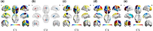
The brain map of the five identified components in the ADNI analysis. (a), (c), (d), and (e) primarily show the cortical regions; (b) shows two subcortical regions, the left and right caudate nucleus.
Comparison between diagnosis groups for females and males and comparison between males and females for each diagnosis group (CN, MCI, and AD) of the five identified components in the ADNI analysis. The numbers in the parentheses are the |$95\%$| confidence intervals obtained from |$500$| bootstrap samples. Significance is highlighted in bold
| Comparison | Group | C1 | C2 | C3 | C4 | C5 |
|---|---|---|---|---|---|---|
| Female | |$\mathbf{0.45~(0.32, ~~0.58)}$| | |$\mathbf{0.69~(0.45, ~~0.92)}$| | |$\mathbf{0.39~(0.26, ~~0.54)}$| | |$0.03~(-0.03, ~~~0.09)$| | |$\mathbf{0.33~(0.20, ~~0.46)}$| | |
| MCI|$-$|CN | Male | |$\mathbf{0.21~(0.09, ~~0.33)}$| | |$\mathbf{-0.48~(-0.90, -0.07)}$| | |$0.22~(-0.01, ~~~0.45)$| | |$\mathbf{0.50~(0.23, ~~0.77)}$| | |$\mathbf{0.54~(0.33, ~~0.76)}$| |
| Female | |$\mathbf{0.31~(0.06, ~~0.56)}$| | |$\mathbf{1.18~(0.71, ~~1.64)}$| | |$\mathbf{0.34~(0.17, ~~0.50)}$| | |$\mathbf{0.43~(0.09, ~~0.78)}$| | |$\mathbf{0.37~(0.08, ~~0.65)}$| | |
| AD|$-$|CN | Male | |$\mathbf{0.18~(0.01, ~~0.34)}$| | |$-0.38~(-0.88, ~~~0.11)$| | |$0.14~(-0.17, ~~~0.44)$| | |$\mathbf{0.40~(0.03, ~~0.77)}$| | |$\mathbf{0.32~(0.08, ~~0.57)}$| |
| Female | |$-0.14~(-0.39, ~~~0.11)$| | |$\mathbf{0.49~(0.05, ~~0.92)}$| | |$-0.06~(-0.20, ~~~0.08)$| | |$\mathbf{0.40~(0.06, ~~0.74)}$| | |$0.04~(-0.25, ~~~0.32)$| | |
| AD|$-$|MCI | Male | |$-0.03~(-0.15, ~~~0.08)$| | |$0.10~(-0.23, ~~~0.44)$| | |$-0.08~(-0.31, ~~~0.14)$| | |$-0.10~(-0.38, ~~~0.18)$| | |$\mathbf{-0.22~(-0.42, -0.02)}$| |
| CN | |$\mathbf{0.22~(0.01, ~~0.45)}$| | |$\mathbf{1.27~(0.76, ~~1.78)}$| | |$0.23~(-0.04, ~~~0.52)$| | |$\mathbf{-0.54~(-0.97, -0.12)}$| | |$\mathbf{-0.40~(-0.70, -0.10)}$| | |
| MCI | |$-0.01~(-0.24, ~~~0.21)$| | |$0.09~(-0.36, ~~~0.55)$| | |$0.05~(-0.21, ~~~0.32)$| | |$-0.07~(-0.43, ~~~0.28)$| | |$-0.19~(-0.46, ~~~0.08)$| | |
| Male|$-$|female | AD | |$0.09~(-0.19, ~~~0.37)$| | |$-0.29~(-0.80, ~~~0.21)$| | |$0.03~(-0.23, ~~~0.30)$| | |$\mathbf{-0.58~(-1.03, -0.12)}$| | |$\mathbf{-0.44~(-0.82, -0.07)}$| |
| Age | |$\mathbf{-0.13~(-0.25, -0.01)}$| | |$\mathbf{-0.32~(-0.56, -0.09)}$| | |$\mathbf{-0.17~(-0.29, -0.05)}$| | |$0.21~(-0.01, ~~~0.42)$| | |$\mathbf{0.17~(0.02, ~~0.32)}$| | |
| Scanner (others) | |$0.15~(-0.04,~~~0.35)$| | |$\mathbf{0.37~(0.13,~~0.61)}$| | |$0.10~(-0.08,~~~0.29)$| | |$0.02~(-0.25,~~~0.30)$| | |$0.05~(-0.18,~~~0.27)$| |
Brain functional modules covered by the five identified components in the ADNI analysis. A “|$\times$|” means that at least one brain region from the module has a nonzero loading in the component
| Visual | Somato-motor | Dorsal-attention | Ventral-attention | Limbic-system | Fronto-parietal | DMN | Subcortical | Cerebellum | |
|---|---|---|---|---|---|---|---|---|---|
| C1 | |$\times$| | |$\times$| | |$\times$| | |$\times$| | |$\times$| | ||||
| C2 | |$\times$| | ||||||||
| C3 | |$\times$| | |$\times$| | |$\times$| | |$\times$| | |||||
| C4 | |$\times$| | |$\times$| | |$\times$| | |$\times$| | |$\times$| | |$\times$| | |||
| C5 | |$\times$| | |$\times$| |
Consistent decrease in DMN connectivity among MCI and AD cohorts has been reported and the findings are robust to the choice of analytical approaches (Badhwar and others, 2017). Regions, such as precentral and postcentral gyri, have been verified to be related to working memory demonstrating the difference in functional connectivity between MCI/AD patients and normal controls (Tomasi and others, 2011). The study of sex differences in brain functional connectivity using fMRI is limited in AD research. In a recent cross-sectional preAD study, functional connectivity in the DMN was found to be lower in males than in females (Cavedo and others, 2018). In a study comparing amnestic MCI and AD with healthy controls, a difference in right caudate nucleus atrophy was observed in females only. Alterations of functional connectivity in the somato-motor, dorsal, and ventral attention networks were identified in male patients (Li and others, 2021). In summary, our findings are in line with existing knowledge about AD.
5. Discussion
In this article, a longitudinal regression model for covariance matrix outcomes is proposed. The proposal considers a multilevel model based on a generalized linear model for covariance matrices to simultaneously identify covariate-associated components, estimate model coefficients, capture the within-subject variation in the covariance matrices, and enable the estimation of individual trajectories. Under the normality assumption, a hierarchical likelihood-based approach is introduced to estimate the parameters. For high-dimensional data, a linear shrinkage estimator of the covariance matrix is introduced. By imposing the shrinkage parameter to be common across visits and subjects, it achieves the optimal property with the uniformly minimum quadratic loss asymptotically among all linear combinations of the identity matrix and the sample covariance matrix. Asymptotic consistency of the estimators is studied for both the low-dimensional and high-dimensional scenarios. Through extensive simulation studies, the proposed approach achieves good performance in identifying the relevant components and estimating the parameters. Applying to a longitudinal resting-state fMRI data set acquired from the ADNI study, the proposed approach identifies brain networks that demonstrate the difference between males and females at different disease stages. The findings are consistent with existing AD research and the method improves the statistical power over the analysis of cross-sectional data.
In this study, it is assumed that the covariate-related component or brain network is constant over time. To support functional dynamics that actuate behavior and cognition through changing demands, reconfiguration of brain networks occurs by compartmentalizing integrated and segregated neural processing of individual brain regions (Khambhati and others, 2018). Thus, future research is to account for the variation in network composition. The current asymptotic theory builds upon the assumption that all the covariance matrices have the same eigenstructure. Though numerical evaluations suggest that this can be relaxed to partial common diagonalization, a thorough theoretical investigation is one future direction. In practice, one can first examine the partial common diagonalization assumption by comparing the eigenvectors across matrices, similar to the procedure performed for the ADNI data set demonstrated in Section D.2 of the Supplementary material available at Biostatistics online. The objective of the proposed approach is to identify projections that are related to the covariates of interest. However, one limitation is that the estimate can be driven by potential confounding effects. In practice, one may consider comparing the results under various model configurations.
In many brain imaging studies, imaging scans are acquired in repeated sessions. One objective of doing so is to examine the test–retest reliability, which quantifies the stability of the repeated measurements. In fMRI studies, a commonly used measure is the intraclass correlation coefficient (ICC, Shrout and Fleiss, 1979), which is defined as the proportion of total variation that can be attributed to the variability between subjects. Converging evidence has shown that univariate measures derived from fMRI studies exhibit a low ICC suggesting poor test–retest reliability (Noble and others, 2019), while multivariate reliability is substantially greater (Noble and others, 2021). For example, the I2C2 showed higher reliability of functional connectivity by pooling together the variance estimates across the brain (Shou and others, 2013). In this vein, the proposed approach may offer a network-level metric of test–retest reliability, where the metric may depend on other covariates, such as the demographic variables. Another potential implementation of the proposed framework is to harmonize imaging data collected at different study sites. It has been shown that correcting for differences in covariance is also essential when analyzing fMRI data (Yu and others, 2018; Yamashita and others, 2019; Chen and others, 2022). The proposed framework can correct for the batch effect across sites by including sites in the regression model.
6. Software
Software in the form of R code, together with a sample input data set and complete documentation are available on GitHub https://github.com/zhaoyi1026/LCAP.
Supplementary material
Supplementary material is available online at http://biostatistics.oxfordjournals.org.
Funding
National Institutes of Health (R01MH126970, P30AG072976, U54AG065181, R01EB029977, P41EB031771, U54DA049110, R01EB022911, RF1AG074204, R01079324).
Acknowledgments
Conflict of Interest: None declared.
