


Summary
In the analysis of single-cell RNA sequencing data, researchers often characterize the variation between cells by estimating a latent variable, such as cell type or pseudotime, representing some aspect of the cell’s state. They then test each gene for association with the estimated latent variable. If the same data are used for both of these steps, then standard methods for computing p-values in the second step will fail to achieve statistical guarantees such as Type 1 error control. Furthermore, approaches such as sample splitting that can be applied to solve similar problems in other settings are not applicable in this context. In this article, we introduce count splitting, a flexible framework that allows us to carry out valid inference in this setting, for virtually any latent variable estimation technique and inference approach, under a Poisson assumption. We demonstrate the Type 1 error control and power of count splitting in a simulation study and apply count splitting to a data set of pluripotent stem cells differentiating to cardiomyocytes.
1. Introduction
Techniques for single-cell RNA sequencing (scRNA-seq) allow scientists to measure the gene expression of huge numbers of individual cells in parallel. Researchers can then investigate how gene expression varies between cells of different states. In particular, we highlight two common questions that arise in the context of scRNA-seq data:
- Question 1.
Which genes are differentially expressed along a continuous cellular trajectory? This trajectory might represent development, activity level of an important pathway, or pseudotime, a quantitative measure of biological progression through a process such as a cell differentiation (Trapnell and others, 2014).
- Question 2.
Which genes are differentially expressed between discrete cell types?
These two questions are hard to answer because typically the cellular trajectory or the cell types are not directly observed, and must be estimated from the data. We can unify these two questions, and many others that arise in the analysis of scRNA-seq data, under a latent variable framework.
Suppose that we have mapped the scRNA-seq reads for |$n$| cells to |$p$| genes (or other functional units of interest). Then, the data matrix |$X$| has dimension |$n \times p$|, and |$X_{ij}$| is the number of reads from the |$i$|th cell that map to the |$j$|th gene. We assume that |$X$| is a realization of a random variable |$\bf{X}$|, and that the biological variation in |${\text{E}}[\bf{X}]$| is explained by a set of latent variables |$L \in \mathbb{R}^{n \times k}$|. We wish to know which columns |$\bf{X}_j$| of |$\bf{X}$| are associated with |$L$|. As |$L$| is unobserved, the following two-step procedure seems natural:
Step 1: Latent variable estimation. Use |$X$| to compute |$\widehat{L}(X)$|, an estimate of |$L$|.
Step 2: Differential expression analysis. For |$j = 1,\ldots,p$|, test for association between |$\bf{X}_j$| and the columns of |$\widehat{L}(X)$|.
In this article, we refer to the practice of using the same data |$X$| to first construct |$\hat{L}(X)$| and second to test for association with |$\hat{L}(X)$| as “double dipping.”
Why is double dipping a problem? As we will see throughout this article, if we use standard statistical tests in Step 2, then we will fail to control the Type 1 error rate. We now provide intuition for this using a very simple motivating example. We generate |$X \in \mathbb{Z}_{\geq 0}^{500 \times 5}$|, where |$\textbf{X}_{ij} \sim \mathrm{Poisson}(5)$| for |$i = 1,\ldots,500$| and |$j=1,\ldots,5$|. The distribution of counts for each of the five genes is shown in the left column of Figure 1. The right panel of Figure 1 shows the result of (1) clustering the data by applying k-means with |$k=2$|, and then (2) testing for association between each gene and the estimated clusters (using a Wald p-value from a Poisson generalized linear model). Even though all cells are drawn from the same distribution, and thus all tested null hypotheses hold, all five p-values are small. The Type 1 error rate is not controlled, because the Wald test does not account for the fact that the clustering algorithm is designed to maximize the difference between the clusters (see the right panel of Figure 1).
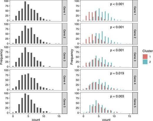
Left: Distributions of counts for five genes under a model where |$\bf{X}_{ij} \sim \mathrm{Poisson}(5)$| for all genes and all cells. Right: Distributions of the same counts, colored by estimated cluster, labeled with the Wald p-values from a Poisson GLM. All p-values are small, despite the fact that all null hypotheses hold.
Despite this issue with double dipping, it is common practice. |$\texttt{Monocle3}$| and |$\texttt{Seurat}$| are popular |$\texttt{R}$| packages that each contain functions for (1) estimating latent variables such as clusters or pseudotime and (2) identifying genes that are differentially expressed across these latent variables. The vignettes for these |$\texttt{R}$| packages perform both steps on the same data (Pliner and others, 2022; Hoffman, 2022). Consequently, the computational pipelines suggested by the package vignettes fail to control the Type 1 error rate. We demonstrate this empirically in Appendix A of the Supplementary material available at Biostatistics online.
Though no suitable solution has yet been proposed, the issues associated with this two-step process procedure are well documented: Lähnemann and others (2020) cite the “double use of data” in differential expression analysis after clustering as one of the “grand challenges” in single cell RNA sequencing (Question 1), and Deconinck and others (2021) note that the “circularity” involved in the two-step process of trajectory analysis leads to “artificially low p-values” for differential expression (Question 2).
In this article, we propose count splitting, a simple fix for the double dipping problem. This allows us to carry out latent variable estimation and differential expression analysis without double dipping, so as to obtain p-values that control the Type 1 error for the null hypothesis that a given gene is not associated with an estimated latent variable.
In Section 2, we introduce the notation and models that will be used in this article. In Section 3, we carefully examine existing methods for latent variable inference and explain why they are not adequate in this setting. In Section 4, we introduce our proposed method, and in Sections 5 and 6, we demonstrate its merits on simulated and real data.
2. Models for scRNA-seq data
Based on (2.1), in this article, we carry out the differential expression analysis step of the two-step process introduced in Section 1 by fitting a generalized linear model (GLM) with a log link function to predict |$X_j$| using |$\widehat{L}(X)$|, with the |$\gamma_i$| included as offsets. We note that while the notation introduced in the remainder of this section is specific to GLMs, the ideas in this article can be extended to accommodate alternate methods for differential expression analysis, such as generalized additive models (as in Van den Berge and others 2020 and Trapnell and others 2014).
Under the model in (2.1), the columns of the matrix |$\log\left(\Lambda\right)$| are linear combinations of the unobserved columns of |$L$|. However, they may not be linear combinations of the estimated latent variables, i.e. the columns of |$\widehat{L}(X)$|. Thus, we need additional notation to describe the population parameters that we target when we fit a GLM with |$\widehat{L}(X)$|, rather than |$L$|, as the predictor.
3. Existing methods for latent variable inference
3.1. Motivating example
Throughout Section 3, we compare existing methods for differential expression analysis after latent variable estimation on a simple example. We generate |$2000$| realizations of |$\bf{X} \in \mathbb{Z}_{\geq 0}^{200 \times 10}$|, where |$\bf{X}_{ij} \overset{\mathrm{ind.}}{\sim} \text{Poisson}(\Lambda_{ij})$|. For |$i = 1,\ldots,200$|, we let |$\Lambda_{ij}=1$| for |$j = 1,\ldots,5$| and |$\Lambda_{ij}=10$| for |$j = 6,\ldots,10$|. (This is an example of the model defined in (2.1) and (2.4) with |$\gamma_1 = \ldots = \gamma_n = 1$| and |$\beta_{1j} = 0$| for |$j = 1,\ldots,10$|.) Under this mechanism, each cell is drawn from the same distribution, and thus there is no true trajectory. Nevertheless, for each data set |$X$|, we estimate a trajectory using the first principal component of the log-transformed data with a pseudocount of one. We then fit Poisson GLMs (with no size factors) to study differential expression. Since all columns of |$\Lambda$| are constant, |$\beta_{1}(Z, \bf{X}_j)=0$| for all |$j$| and for any |$Z \in \mathbb{R}^n$| (see (2.2)). Therefore, any p-value quantifying the association between a gene and an estimated trajectory should follow a |$\text{Unif}(0,1)$| distribution. As we will see, most available approaches do not have this behavior.
3.2. The double dipping method
The right-hand side of the inequality in (3.5) uses the observed data to obtain both the predictor and the response, while the left-hand side does not. Thus, |$\widehat{\beta}_{1}\left(\widehat{L}(X),X_j\right)$| is drawn from |$\widehat{\beta}_{1}\left(\widehat{L}(\bf{X}),\bf{X}_j\right)$|, not |$\widehat{\beta}_{1}\left(\widehat{L}(X),\bf{X}_j\right)$|. To state the issue in a different way, we used the data realization |$X$| to construct both the predictor |$\hat{L}(X)$| and the response |$X_j$| in the GLM, and did not account for this double use in determining the distribution of the test statistic. Therefore, as shown in Figure 2(a), when we compute the p-value in (3.5) for many realizations of |$\bf{X}$|, the collection of p-values does not follow a |$\text{Unif}(0,1)$| distribution.
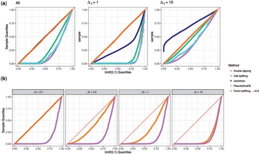
Uniform QQ-plots of p-values under the null. (a): The data are Poisson. p-values are displayed for the |$p=10$| genes in each of 2000 data sets generated as described in Section 3.1. The left-hand panel shows all of the genes aggregated, whereas the center and right panels break the results down by the value of |$\Lambda_{ij}$|. (b): The data are negative binomial. p-values are displayed for the |$p=10$| genes in each data set for the simulation described in Section 4.2. Results are broken down by the magnitude of |$\frac{\Lambda}{b}$|. As |$\frac{\Lambda}{b}$| increases, the correlation between |$\bf{X}^{\mathrm{train}}$| and |$\bf{X}^{\mathrm{test}}$| increases, and the performance of count splitting approaches that of the double dipping method.
3.3. Cell splitting
In some settings, it is possible to overcome the issues associated with double dipping by splitting the observations into a training set and a test set, generating a hypothesis on the training set, and testing it on the test set (Cox, 1975). However, in the setting of this article, splitting the cells in |$X$| does not allow us to bypass the issues of double dipping.
Why not? Suppose we estimate the latent variables using the cells in the training set, |$X^{\mathrm{train}}$|. To test for differential expression using the cells in |$X^{\mathrm{test}}$|, we need latent variable coordinates for the cells in |$X^{\mathrm{test}}$|. However, it is not clear how to obtain latent variable coordinates for the cells in |$X^\mathrm{test}$| that are only a function of the training set and not the test set (i.e. can be written as |$\widehat{L}(X^\mathrm{train})$|). In the simple example from Section 3.1, after computing the first principal axis of the log-transformed |$X^{\mathrm{train}}$| matrix, we could consider projecting the log-transformed |$X^{\mathrm{test}}$| onto this axis to obtain coordinates for the cells in |$X^{\mathrm{test}}$|. Unfortunately, this projection step uses the data in |$X^{\mathrm{test}}$|, and so the resulting estimated coordinates must be written as |$\widehat{L}\left(X^\mathrm{train}, X^\mathrm{test}\right)$|.
Unfortunately, (3.6) suffers from the same issue as (3.5): the right-hand side of the inequality uses the same realization (|$X^\mathrm{test}$|) to construct both the predictor and the response, whereas the left-hand side does not. Thus, the p-values from (3.6) do not follow a |$\text{Unif}(0,1)$| distribution, even when the columns of |$\Lambda$| are constants. Instead, they are anti-conservative, as shown in Figure 2(a).
3.4. Gene splitting
As the coefficients on the right-hand side of these inequalities never use the same data to construct the predictor and the response, these p-values will be uniformly distributed over repeated realizations of |$\bf{X}$| when the columns of |$\Lambda$| are constants. However, they are fundamentally unsatisfactory in scRNA-seq applications where we wish to obtain a p-value for every gene with respect to the same estimated latent variable. Thus, gene splitting is not included in Figure 2(a).
3.5. Selective inference through conditioning
The approach in (3.7) is not suitable for the setting of this article. First, (3.7) cannot be computed in practice. The selective inference literature typically modifies (3.7) by conditioning on extra information for computational tractability. Conditioning on extra information does not sacrifice Type 1 error control, and the extra information can be cleverly chosen such that the modified p-value is simple to compute under a multivariate normality assumption. Because scRNA-seq data consists of non-negative integers, a normality assumption is not suitable, and so this approach does not apply. Second, as the conditioning event in (3.7) must be explicitly characterized, each choice of |$\widehat{L}(\cdot)$| will require its own bespoke strategy. This is problematic in the scRNA-seq setting, where many specialized techniques are used for pre-processing, clustering, and trajectory estimation. Zhang and others (2019) overcome this challenge in the context of clustering by combining cell splitting (Section 3.3) with selective inference. The idea is to condition on the test set labeling event |$\left\{ \widehat{L}\left(X^{\mathrm{train}}, \bf{X}^\mathrm{test}\right) = \widehat{L}\left(X^{\mathrm{train}}, X^{\mathrm{test}}\right) \right\}$|, which can be characterized provided that the estimated clusters are linearly separable. However, their work requires a normality assumption and does not extend naturally to the setting of trajectory estimation.
Selective inference is omitted as a comparison method in Figure 2(a) because we are not aware of a way to compute (3.7) for Poisson data, even for our simple choice for |$\widehat{L}\left(\cdot\right)$|. In Appendix C of the Supplementary material available at Biostatistics online, we show that the selective inference method of Gao and others (2022), which provides finite-sample valid inference after clustering for a related problem under a normality assumption, does not control the Type 1 error rate when applied to log-transformed Poisson data.
3.6. Jackstraw
Under the null hypothesis that |$\beta_{1j} = 0$| in (3.9), |$X^\mathrm{permute,b}$| and |$X$| have the same distribution. Furthermore, both sides of the inequality in (3.10) use the same data realization to construct the predictor and the response. This suggests that under the null hypothesis that |$\beta_{1j}=0$| in (3.9), the distribution of the p-value in (3.10) will converge to |$\text{Unif}(0,1)$| as |$B \rightarrow \infty$|. This null hypothesis is slightly different than the ones tested in Sections 3.2–3.5, which involved association between the |$j$|th gene and an estimated latent variable.
Since all |$p$| genes are compared to the same reference distribution, only |$B$| total computations of |$\widehat{L}(\cdot)$| are needed. Unfortunately, the p-value in (3.11) only follows a |$\text{Unif}(0,1)$| distribution if the quantity on the right-hand side of the inequality in (3.11) follows the same distribution for |$j=1,\ldots,p$|. This does not hold in the simple example from Section 3.1, where the quantity has a different distribution for the genes with |$\Lambda_{ij}=1$| than those with |$\Lambda_{ij}=10$|. While the collection of p-values aggregated across all of the genes appears to follow a |$\text{Unif}(0,1)$| distribution (Figure 2(a), left), some genes have anti-conservative p-values (Figure 2(a), center) and others have overly conservative p-values (Figure 2(a), right).
3.7. PseudotimeDE
While it is not entirely clear what null hypothesis PseudotimeDE is designed to test, we can see that there is a problem with the p-value in (3.12). On the right-hand side of the inequality in (3.12), there is association between the predictor and the response in the GLM due to the fact that both are generated from the data |$X$|. On the left-hand side of the inequality in (3.12), permuting |$\widehat{L}(X^b)$| disrupts the association between the predictor and the response. Thus, even in the absence of any signal in the data, the quantity on the right-hand side of (3.12) does not have the same distribution as the quantity on the left-hand side of (3.12). As shown in Figure 2(a), under our simple example where there is no true trajectory, the p-values from (3.12) are anti-conservative.
4. Count splitting
4.1. Method
In Sections 3.3 and 3.4, we saw that cell splitting and gene splitting are not suitable options for latent variable inference on scRNA-seq data. Here, we propose count splitting, which involves splitting the expression counts themselves, rather than the genes or the cells, to carry out latent variable estimation and differential expression analysis. The algorithm is as follows.
(Count splitting for latent variable inference) For a constant |$\epsilon$| with |$0 < \epsilon < 1$|,
- Step 0: Count splitting.
Draw |$\bf{X}^{\mathrm{train}}_{ij} \mid \{\bf{X}_{ij} = X_{ij} \} \overset{\mathrm{ind.}}{\sim} \mathrm{Binomial}\left(X_{ij}, \epsilon\right)$|, and let |$X^{\mathrm{test}} = X-X^{\mathrm{train}}$|.
- Step 1: Latent variable estimation.
Compute |$\widehat{L}\left(X^{\mathrm{train}}\right)$|.
- Step 2: Differential expression analysis.
For |$j = 1,\ldots,p$|,
- (a)
Fit a GLM with a log link to predict |$X^{\mathrm{test}}_j$| using |$\widehat{L}(X^{\mathrm{train}})$|, with the |$\gamma_i$| included as offsets. This provides |$\widehat{\beta}_1\left( \widehat{L}\left(X^{\mathrm{train}}\right), {X}_j^\mathrm{test}\right)$|, an estimate of |$\beta_1\left( \widehat{L}\left(X^{\mathrm{train}}\right), \bf{X}_j^\mathrm{test}\right)$|.
- (b)Compute a Wald p-value for |$H_0: \beta_1\left( \widehat{L}\left(X^{\mathrm{train}}\right), \bf{X}_j^\mathrm{test}\right)=0$| vs. |$H_1: \beta_1\left( \widehat{L}\left(X^{\mathrm{train}}\right), \bf{X}_j^\mathrm{test}\right) \neq 0$|, which takes the form(4.13)$$\begin{equation} \label{eq_countsplitp} Pr_{H_0:\ \beta_1\left(\widehat{L}(X^{\mathrm{train}}),\bf{X}^\mathrm{test}_j\right)=0} \left( \left| \widehat{\beta}_{1}\left(\widehat{L}({X}^\mathrm{train}),\bf{X}^\mathrm{test}_j\right) \right| \geq \left| \widehat{\beta}_{1}\left(\widehat{L}\left(X^{\mathrm{train}}\right), X_j^\mathrm{test}\right) \right| \right)\!. \end{equation}$$
- (a)
Note that in Step 2(b), we are computing a standard GLM Wald p-value for a regression of |$X_j^\mathrm{test}$| onto |$\widehat{L}(X^{\mathrm{train}})$|. The next result is a well-known property of the Poisson distribution.
(Binomial thinning of Poisson processes (see Durrett 2019, Section 3.7.2)) If |$\bf{X}_{ij} \sim {\rm Poisson}(\gamma_i \Lambda_{ij})$|, then |$\bf{X}_{ij}^\mathrm{train}$| and |$\bf{X}_{ij}^\mathrm{test}$|, as constructed in Algorithm 1, are independent. Furthermore, |$\bf{X}_{ij}^\mathrm{train} \sim {\rm Poisson}(\epsilon \gamma_i \Lambda_{ij})$| and |$\bf{X}_{ij}^\mathrm{test} \sim {\rm Poisson}((1-\epsilon) \gamma_i \Lambda_{ij})$|.
This means that in (4.13), under a Poisson model, the predictor and the response are independent on both sides of the inequality. Consequently, the p-value in (4.13) will retain all standard properties of a GLM Wald p-value: for example, control of the Type 1 error rate for |$H_0:\ \beta_1\left(\widehat{L}(X^{\mathrm{train}}),\bf{X}^\mathrm{test}_j\right)=0,$| when |$n$| is sufficiently large. Furthermore, when |$n$| is sufficiently large, we can invert the test in (4.13) to obtain confidence intervals with |$100\times(1-\alpha)\%$| coverage for the parameter |$\beta_1\left(\widehat{L}(X^{\mathrm{train}}),\bf{X}^\mathrm{test}_j\right)$|.
We now consider the parameter |$\beta_1\left(\widehat{L}(X^{\mathrm{train}}),\bf{X}^\mathrm{test}_j\right)$|. Suppose that for any matrix |$M$| and scalar |$a$|, the function |$\widehat{L}(\cdot)$| satisfies |$\widehat{L}(aM) \propto \widehat{L}(M)$|. In this case, Proposition 1 says that |$\widehat{L}\left( E[\bf{X}^{\mathrm{train}}]\right) = \widehat{L}\left( \epsilon E[\bf{X}] \right) \propto \widehat{L}\left(E[\bf{X}]\right)$|. Furthermore, if |$\log\left( E[\bf{X}_j]\right) = \beta_0 + \beta_1^T L_i$|, then |$\log\left(E[\bf{X}^\mathrm{test}_j]\right) = \log(1-\epsilon) + \beta_0 + \beta_1^T L_i.$| Therefore, |$\beta_1\left(\widehat{L}(X^{\mathrm{train}}),\bf{X}^\mathrm{test}_j\right)$| is closely related to |$\beta_1\left(\widehat{L}(X),\bf{X}_j\right)$|, the parameter (unsuccessfully) targeted by the double dipping method (Section 3.2).
The key insight behind Algorithm 1 is that, under a Poisson assumption, a test for association between |$\widehat{L}\left(X^\mathrm{train}\right)$| and |$\bf{X}_j^\mathrm{test}$| that uses |$\widehat{L}\left(X^\mathrm{train}\right)$| and |$X_j^\mathrm{test}$| will inherit standard statistical guarantees, despite the fact that |$\widehat{L}\left(X^\mathrm{train}\right)$| and |$X_j^\mathrm{test}$| are functions of the same data. This insight did not rely on the use of a GLM or a Wald test in Step 2 of Algorithm 1. Thus, other approaches could be used to quantify this association.
Figure 2(a) shows that count splitting with |$\epsilon=0.5$| produces uniformly distributed p-values for all genes in the example described in Section 3.1, using a Poisson GLM in Step 2 of Algorithm 1. We explore more values of |$\epsilon$| and more complicated scenarios in Section 5.
Count splitting is a special case of “data fission”, proposed in a preprint by Leiner and others (2022) while this article was in preparation. While the data fission framework is broad enough to encompass this latent variable setting, Leiner and others (2022) focus on comparing data fission to sample splitting in supervised settings where the latter is an option. In unsupervised settings, where sample splitting is not an option (as seen in Section 3.3), ideas similar to count splitting have been applied by Batson and others (2019) and Chen and others (2021) for tasks such as evaluating the goodness-of-fit of a low-rank approximation of a matrix. We elaborate on connections to Batson and others (2019) in Appendix B of the Supplementary material available at Biostatistics online. Finally, Gerard (2020) suggests applying binomial thinning to real scRNA-seq data sets to generate synthetic data sets to use for comparing and evaluating scRNA-seq software packages and methods, and this approach is used in the supplement of Sarkar and Stephens (2021) to compare various scRNA-seq models.
4.2. What if the data are not Poisson?
The independence between |$\bf{X}_{ij}^\mathrm{train}$| and |$\bf{X}_{ij}^\mathrm{test}$| in Proposition 1 holds if and only if |$\bf{X}_{ij}$| has a Poisson distribution (Kimeldorf and others, 1981). Thus, if we apply Algorithm 1 to data that are not Poisson, there will be dependence between the predictor and the response on the right-hand side of the inequality in (4.13), and the p-value in (4.13) will not be uniformly distributed under |$H_0$|.
Wang and others (2018) argue that the Poisson model is sufficient to model scRNA-seq data. Townes and others (2019) advocate modeling the counts for each cell with a multinomial distribution. When the number of genes is large, the elements of the multinomial can be well-approximated by independent Poisson distributions, and indeed the authors rely on this approximation for computational reasons. Similarly, Batson and others (2019) assume that |$\bf{X}_{ij} \sim \mathrm{Binomial}(\Omega_{ij}, p_i)$|, but note that typically |$\Omega_{ij}$| is large and |$p_i$| is small, so that a Poisson approximation applies.
To investigate the performance of count splitting under overdispersion, we generate data sets under (4.14) with |$n=200$| and |$p=10$|. For each data set, |$\Lambda_{ij} = \Lambda = 5$| for |$i=1,\ldots,n$| and |$j=1,\ldots,p$|, and |$b_j=b$| for |$j=1,\ldots,p$|, so that every element of |$X$| is drawn from the same distribution. We generate 500 data sets for each value of |$b \in \{50,10,5,0.5\}$|, so that |$\frac{\Lambda}{b} \in \{0.1, 0.5, 1, 10\}$|. Figure 2(b) displays the Wald p-values that result from running Algorithm 1 with a negative binomial GLM in Step 2, for all genes across all of the simulated datasets.
The denominator of (4.15) in Proposition 2 shows that |$\frac{\Lambda}{b}$| determines the extent of correlation between |$\bf{X}^{\mathrm{train}}$| and |$\bf{X}^{\mathrm{test}}$| in this setting. As shown in Figure 2(b), when |$\frac{\Lambda}{b}$| is small, count splitting produces approximately uniformly distributed p-values and thus comes very close to controlling the Type 1 error rate. As |$\frac{\Lambda}{b}$| grows, the performance of count splitting approaches that of the double dipping method discussed in Section 3.2. Thus, count splitting tends to outperform the double dipping method, and in the case of extremely high overdispersion will be no worse than the double dipping method. For the real scRNA-seq data set considered in Section 6, we show in Appendix F of the Supplementary material available at Biostatistics online that the majority of the estimated values of |$\frac{\Lambda_{ij}}{b_j}$| are less than |$1$|.
4.3. Choosing the tuning parameter |$\epsilon$|
The parameter |$\epsilon$| in Algorithm 1 governs a tradeoff between the information available for estimating |$L$| and the information available for carrying out inference. Proposition 3, proven in Appendix E of the Supplementary material available at Biostatistics online, formalizes the intuition that |$X^{\mathrm{train}}$| will look more similar to |$X$| when |$\epsilon$| is large.
If |$\bf{X}_{ij} \sim \mathrm{Poisson}(\gamma_i \Lambda_{ij})$|, then |$\mathrm{Cor}(\bf{X}_{ij}, \bf{X}_{ij}^\mathrm{train}) = \sqrt{\epsilon}.$|
Thus, as |$\epsilon$| decreases, we expect |$\widehat{L}(X^{\mathrm{train}})$| and |$\widehat{L}(X)$| to look less similar. This is a drawback, as scientists would ideally like to estimate |$L$| using all of the data. However, as |$\epsilon$| increases, the power to reject false null hypotheses in Step 2(b) of Algorithm 1 decreases. Proposition 4, proven in Appendix E of the Supplementary material available at Biostatistics online, quantifies this loss of power.
Let |$\bf{X}_{ij} \overset{\mathrm{ind.}}{\sim} \mathrm{Poisson}\left( \gamma_i \exp(\beta_{0j} +\beta_{1j} L_i )\right)$|. Then |$\text{Var}\left(\widehat{\beta}_1(L, \bf{X}^\mathrm{test}_j)\right) \approx \frac{1}{1-\epsilon} \text{Var}\left(\widehat{\beta}_1(L, \bf{X}_j)\right)\!.$|
In the ideal setting where |$\widehat{L}(X^{\mathrm{train}})=L$| and |$L \in \mathbb{R}^{n \times 1}$| for simplicity, using |$\bf{X}_j^\mathrm{test}$| rather than |$\bf{X}_j$| as the response inflates the variance of the estimated coefficient by a factor of |$\frac{1}{1-\epsilon}$|. Thus, when |$\epsilon$| is large, Step 2(b) of Algorithm 1 has lower power. In practice, we recommend setting |$\epsilon=0.5$| to balance the dual goals of latent variable estimation and downstream inference.
5. Simulation study
5.1. Data-generating mechanism
We generate data from (2.1) and (2.4) with |$n=2700$| and |$p=2000$|. We generate the size factors |$\gamma_i \overset{\mathrm{ind.}}{\sim} \text{Gamma}\left(10, 10\right)$| and treat them as known. Throughout this section, whenever we perform count splitting, we fit a Poisson GLM in Step 2 of Algorithm 1 and report Wald p-values.
In this section, we investigate the performance of count splitting under two data-generating mechanisms: one generates a true continuous trajectory and the other generates true clusters. To generate data with an underlying trajectory, we set |$L = \left(I_n - \frac{1}{n} 11^T\right) Z$|, where |$Z_i \overset{\mathrm{ind.}}{\sim} N(0,1)$|. Under (2.1), |$L$| is the first principal component of the matrix |$\log(\Lambda)$|. To estimate |$L$|, we take the first principal component of the matrix |$\log(\text{diag}(\gamma)^{-1} X + 11^T)$|. To generate data with underlying cell types, we let |$L_i \overset{\mathrm{ind.}}{\sim}\text{Bernoulli}(0.5)$| in (2.1), indicating membership in one of two cell types. We estimate |$L$| by running |$k$|-means with |$k=2$| on the matrix |$\log\left (\text{diag}(\gamma)^{-1} X + 11^T\right)$|. (In each case, we have used a pseudocount of one to avoid taking the log of zero.)
In our primary simulation setting, the value |$\beta_{0j}$| for each gene is randomly chosen to be either |$\log(3)$| or |$\log(25)$| with equal probability, such that the data includes a mix of low-intercept and high-intercept genes. For each data set, we let |$\beta_{1j}=0$| for |$90\%$| of the |$p$| genes. Under (2.1), |$\Lambda_{1j} = \ldots = \Lambda_{nj}$| for these genes and thus |$\beta_1\left(Z, \bf{X}_j \right)=0$| for any estimated latent variable |$Z$|. Thus, we refer to these as the null genes. The remaining 10|$\%$| of the genes have the same non-zero value of |$\beta_{1j}$|; these are the differentially expressed genes. For each latent variable setting, we generate |$100$| data sets for each of 15 equally spaced values of |$\beta_{1j}$| in |$[0.18, 3]$|.
5.2. Type 1 error results
Figure 3(a) shows that count splitting controls the Type 1 error rate for a range of |$\epsilon$| values for the 90|$\%$| of genes for which |$\beta_{1j}=0$| in data sets that are generated as specified in Section 5.1.
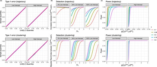
(a) Uniform QQ plots of GLM p-values for all null genes from the simulations described in Section 5.1. (b) Quality of estimate of |$L$|, as defined in Section 5.3, as a function of |$\beta_{1j}$| and the percent of low-intercept genes in the data set. (c) The proportion of null hypotheses that are rejected, aggregated across all non-null genes for all data sets generated with 50|$\%$| low-intercept and 50|$\%$| high-intercept genes. The parameter |$\beta_1\left(\hat{L}(X^\mathrm{train}), \bf{X}_j^\mathrm{test}\right)$| is defined in (2.2).
5.3. Quality of estimate of |$L$|
As mentioned in Section 4.3, smaller values of |$\epsilon$| in count splitting compromise our ability to accurately estimate the unobserved latent variable |$L$|. To quantify the quality of our estimate of |$L$|, in the trajectory estimation case, we compute the absolute value of the correlation between |$L$| and |$\widehat{L}\left(X^{\mathrm{train}}\right)$|, and in the clustering setting, we compute the adjusted Rand index (Hubert and Arabie, 1985) between |$L$| and |$\widehat{L}\left(X^{\mathrm{train}}\right)$|. The results are shown in Figure 3(b). Here, we consider three settings for the value of |$\beta_{0j}$|: (i) each gene is equally likely to have |$\beta_{0j}=\log(3)$| or |$\beta_{0j}=\log(25)$| (as in Section 5.2); (ii) all genes have |$\beta_{0j}=\log(3)$| (“100|$\%$| low-intercept” setting); and (iii) all genes have |$\beta_{0j}=\log(25)$| (“100|$\%$| high-intercept” setting). The 100|$\%$| low-intercept setting represents a case where the sequencing was less deep, and thus the data more sparse.
After taking a log transformation, the genes with |$\beta_{0j}=\log(3)$| have higher variance than those with |$\beta_{0j}=\log(25)$|. Thus, there is more noise in the “100|$\%$| low-intercept” setting than in the “100|$\%$| high-intercept” setting. As a result, for a given value of |$\epsilon$|, the “100|$\%$| low-intercept” setting results in the lowest-quality estimate of |$L$|. Estimation of |$L$| is particularly poor in the “100|$\%$| low-intercept” setting when |$\epsilon$| is small, since then |$X^{\mathrm{train}}$| contains many zero counts. This suggests that count splitting, especially with small values of |$\epsilon$|, is less effective on shallow sequencing data.
5.4. Power results
For each data set and each gene, we compute the true parameter |$\beta_{1}\left(\widehat{L}\left(X^{\mathrm{train}}\right), \bf{X}_j^\mathrm{test}\right)$| defined in (2.2). For a Poisson GLM (i.e., |$p_\theta(\cdot)$| in (2.2) is the density of a |$\mathrm{Poisson}(\theta)$| distribution), it is straightforward to show that we can compute |$\beta_{1}\left(\widehat{L}\left(X^{\mathrm{train}}\right), \bf{X}_j^\mathrm{test}\right)$| by fitting a Poisson GLM with a log link to predict |$E\left[ \bf{X}_{j} \right]$| using |$\widehat{L}\left(X^\mathrm{train}\right)$|, with the |$\gamma_i$| included as offsets.
Figure 3(c) shows that our ability to reject the null hypothesis depends on this true parameter, as well as on the value of |$\epsilon$|. These results are shown in the setting where 50|$\%$| of the genes have intercept |$\log(3)$| and the other 50|$\%$| have intercept |$\log(25)$|. The impact of |$\epsilon$| on power is more apparent for genes with smaller intercepts, as these genes have even less information left over for inference when |$(1-\epsilon)$| is small. This result again suggests that count splitting will work best on deeply sequenced data where expression counts are less sparse.
As suggested by Section 4.3, Figures 3(a) and (c) show a tradeoff in choosing |$\epsilon$|: a larger value of |$\epsilon$| improves latent variable estimation but yields lower power for differential expression analysis. In practice, we recommend choosing |$\epsilon=0.5$|.
5.5. Coverage results
For each data set and each gene, we compute a 95|$\%$| Wald confidence interval for the slope parameter in the GLM. As shown in Table 1, these intervals achieve nominal coverage for the target parameter |$\beta_{1}\left(\widehat{L}\left(X^{\mathrm{train}}\right), \bf{X}_j^\mathrm{test}\right)$|, defined in (2.2) and computed as in Section 5.4.
The proportion of 95|$\%$| confidence intervals that contain |$\beta_{1}\left(\widehat{L}\left(X^{\mathrm{train}}\right), \bf{X}_j^\mathrm{test}\right)$|, aggregated across genes and across values of |$\epsilon$|
| Trajectory estimation | Clustering | |||||
|---|---|---|---|---|---|---|
| Low intercept | High intercept | Low intercept | High intercept | |||
| Null genes | 0.950 | 0.950 | 0.949 | 0.950 | ||
| Non-null genes | 0.955 | 0.956 | 0.949 | 0.950 | ||
| Trajectory estimation | Clustering | |||||
|---|---|---|---|---|---|---|
| Low intercept | High intercept | Low intercept | High intercept | |||
| Null genes | 0.950 | 0.950 | 0.949 | 0.950 | ||
| Non-null genes | 0.955 | 0.956 | 0.949 | 0.950 | ||
6. Application to cardiomyocyte differentiation data
Elorbany and others (2022) collect single-cell RNA sequencing data at seven unique time points (over 15 days) in 19 human cell lines. The cells began as induced pluripotent stem cells (IPSCs) on Day 0, and over the course of 15 days they differentiated along a bifurcating trajectory into either cardiomyocytes (CMs) or cardiac fibroblasts (CFs). We are interested in studying genes that are differentially expressed along the trajectory from IPSC to CM. Throughout this analysis, we ignore the true temporal information (the known day of collection).
Starting with the entire data set |$X$|, we first perform count splitting with |$\epsilon=0.5$| to obtain |$X^\mathrm{train}$| and |$X^\mathrm{test}$|. We then perform the lineage estimation task from Elorbany and others (2022) on |$\mathrm{X}^\mathrm{train}$| to come up with a subset of 10 000 cells estimated to lie on the IPSC to CM trajectory. We retain only these 10 000 cells for further analysis. In what follows, to facilitate comparison between the double dipping method and our count splitting approach, we will use this same subset of 10 000 cells for all methods, even though in practice the double dipping method would have chosen the lineage subset based on all of the data, rather than on |$X^\mathrm{train}$| alone.
Next, we estimate a continuous differentiation trajectory using the |$\texttt{orderCells()}$| function from the |$\texttt{Monocle3}$| package in |$\texttt{R}$| (Pliner and others, 2022). Details are given in Appendix G of the Supplementary material available at Biostatistics online. To estimate the size factors |$\gamma_1,\ldots,\gamma_n$| in (2.4), we let |$\hat{\gamma}_i(X)$| be the normalized row sums of the expression matrix |$X$|, as is the default in the |$\texttt{Monocle3}$| package. Throughout this section, for |$j=1,\ldots,p$|, we compare three methods:
- Full double dipping:
Fit a Poisson GLM of |$X_j$| on |$\widehat{L}(X)$| with |$\hat{\gamma}_i(X)$| included as offsets.
- Count splitting:
Fit a Poisson GLM of |$X^\mathrm{test}_j$| on |$\widehat{L}(X^\mathrm{train})$| with |$\hat{\gamma}_i(X^\mathrm{train})$| included as offsets.
- Test double dipping:
Fit a Poisson GLM of |$X^\mathrm{test}_j$| on |$\widehat{L}(X^\mathrm{test})$| with |$\hat{\gamma}_i(X^\mathrm{test})$| included as offsets.
For each method, we report the Wald p-values for the slope coefficients. The test double dipping method is included to facilitate understanding of the results from the other two methods. We show in Appendix F of the Supplementary material available at Biostatistics online that the estimated overdispersion parameters are relatively small for this data set, justifying the use of count splitting and Poisson GLMs in each of the methods above. In conducting count splitting, we ensure that none of the pre-processing steps required to compute |$\widehat{L}(X^\mathrm{train})$| make use of |$X^\mathrm{test}$|.
We first analyze all |$10\,000$| cells. There is a true differentiation trajectory in this data set: cells were sampled at seven different time points of a directed differentiation protocol, and changes in gene expression as well as phenotype that are characteristic of this differentiation process were observed (Elorbany and others, 2022). We focus on a subset of |$p=2500$| high-variance genes that were selected from more than |$32 \,000$| genes that were expressed in the raw data (see Appendix G of the Supplementary material available at Biostatistics online for details). The left panel of Figure 4 displays the count splitting p-values for differential expression of these 2500 genes against the double dipped p-values.
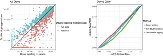
Left: Count splitting p-values vs. double dipped p-values for |$2500$| genes, on a log scale, when all |$10\,000$| cells are used in the analysis. Right: Uniform QQ plot of p-values for |$2500$| genes obtained from each method when only the Day 0 cells are used.
We first note the general agreement between the three methods: genes that have small p-values with one method generally have small p-values with all the methods. Thus, count splitting tends to identify the same differentially expressed genes as the methods that double dip when there is a true trajectory in the data. That said, we do notice that the full double dipping method tends to give smaller p-values than count splitting. There are two possible reasons for this: (i) the double dipped p-values may be artificially small due to the double dipping, or (ii) it might be due to the fact that the full double dipping method uses twice as much data. In this setting, it seems that (ii) is the correct explanation: the test double dipping method (which uses the same amount of data as count splitting both to estimate |$L$| and to test the null hypothesis) does not yield smaller p-values than count splitting. It seems that there is enough true signal in this data that most of the genes identified by the double dipped methods as differentially expressed are truly differentially expressed, rather than false positives attributable to double dipping.
Next, we subset the 10 000 cells to only include the |$2303$| cells that were measured at Day |$0$| of the experiment, before differentiation had begun. Then, despite knowing that these cells should be largely homogeneous, we apply |$\widehat{L}(\cdot)$| to estimate pseudotime. We note that the |$\widehat{L}(\cdot)$| function described in Appendix G of the Supplementary material available at Biostatistics online controls for cell cycle-related variation in gene expression so that this signal cannot be mistaken for pseudotime. We suspect that in this setting, any association seen between pseudotime and the genes is due to overfitting or random noise. We select a new set of |$2500$| high-variance genes using this subset of cells. The right panel of Figure 4 shows uniform QQ plots of the p-values for these |$2500$| genes from each of the three methods. In the absence of real differentiation signal, the p-values should follow a uniform distribution. We see that count splitting controls the Type 1 error rate, while the methods that double dip does not. Unlike the previous example that had a very strong true differentiation signal, even test double dipping yields false positives. Without assessment, the level of true signal in any data set cannot be assumed to outweigh the effects of double dipping.
In summary, count splitting detects differentially expressed genes when there is true signal in the data and protects against Type 1 errors when there is no true signal in the data.
7. Discussion
Under a Poisson assumption, count splitting provides a flexible framework for carrying out valid inference after latent variable estimation that can be applied to virtually any latent variable estimation method and inference technique. This has important applications in the growing field of pseudotime or trajectory analysis, as well as in cell type analysis.
We expect count splitting to be useful in situations other than those considered in this article. For example, as explored in Appendix C of the Supplementary material available at Biostatistics online, count splitting can be used to test the overall difference in means between two estimated clusters, as considered by Gao and others (2022). As suggested in related work by Batson and others (2019), Chen and others (2021), and Gerard (2020), count splitting could be used for model selection tasks such as choosing how many dimensions to keep when reducing the dimension of Poisson scRNA-seq data. Finally, count splitting may lead to power improvements over sample splitting for Poisson data on tasks where the latter is an option (Leiner and others, 2022).
In this article, we assume that after accounting for heterogenous expected expression across cells and genes, the scRNA-seq data follow a Poisson distribution. Some authors have argued that scRNA-seq data are overdispersed. As discussed in Section 4.2, count splitting fails to provide independent training and testing sets when applied to negative binomial data. Leiner and others (2022) suggest that inference can be carried out in this setting by working with the conditional distribution of |$X^\mathrm{test} \mid X^{\mathrm{train}}$|. Unfortunately, this conditional distribution does not lend itself to inference on parameters of interest. In future work, we will consider splitting algorithms for overdispersed count distributions.
Code for reproducing the simulations and real data analysis in this article is available at |$\texttt{github.com/anna-neufeld/countsplit_paper}$|. An |$\texttt{R}$| package with tutorials is available at |$\texttt{anna-neufeld.github.io/countsplit}$|.
Supplementary material
Supplementary material is available at http://biostatistics.oxfordjournals.org.
Acknowledgments
Conflict of Interest: None declared.
Funding
The Simons Foundation (NIH R01 EB026908, NIH R01 GM123993, NIH R01 DA047869, Simons Investigator Award in Mathematical Modeling of Living Systems) to A.N. and D.W.; the Natural Sciences and Engineering Research Council of Canada (Discovery Grants) to L.G.; NIGMS MIRA - 1R35GM139580 to A.B.
