


Summary
Trial-level surrogates are useful tools for improving the speed and cost effectiveness of trials but surrogates that have not been properly evaluated can cause misleading results. The evaluation procedure is often contextual and depends on the type of trial setting. There have been many proposed methods for trial-level surrogate evaluation, but none, to our knowledge, for the specific setting of platform studies. As platform studies are becoming more popular, methods for surrogate evaluation using them are needed. These studies also offer a rich data resource for surrogate evaluation that would not normally be possible. However, they also offer a set of statistical issues including heterogeneity of the study population, treatments, implementation, and even potentially the quality of the surrogate. We propose the use of a hierarchical Bayesian semiparametric model for the evaluation of potential surrogates using nonparametric priors for the distribution of true effects based on Dirichlet process mixtures. The motivation for this approach is to flexibly model relationships between the treatment effect on the surrogate and the treatment effect on the outcome and also to identify potential clusters with differential surrogate value in a data-driven manner so that treatment effects on the surrogate can be used to reliably predict treatment effects on the clinical outcome. In simulations, we find that our proposed method is superior to a simple, but fairly standard, hierarchical Bayesian method. We demonstrate how our method can be used in a simulated illustrative example (based on the ProBio trial), in which we are able to identify clusters where the surrogate is, and is not useful. We plan to apply our method to the ProBio trial, once it is completed.
1. Introduction
Confirmatory randomized clinical trials should be based on clinical endpoints such as death or cure. However, these outcomes can take a long time to observe increasing both the cost and time to approval of new, and potentially effective, treatment strategies. Trial-level surrogates, termed trial-level general surrogates in Gabriel and others (2016), that have been properly evaluated can be used to decrease the length and cost of trials by being used as replacement endpoints. Such endpoints are particularly useful in Phase II and IIb trials, where new treatments of strategies are being evaluated prior to final rigorous testing in a Phase III study. Gabriel and others (2016, 2019) both used examples from multiple trials to evaluate the Zoster vaccine; the trials had differing protocols, were conducted in different countries, and were approximately independent that allowed a trial-level surrogate analysis. However, this was a massive data collection effort that is likely not feasible in most situations.
Platform trials are becoming more common in studies of cancer treatment (Meyer and others, 2020) and will likely become even more common in chronic illness settings. These trials offer a useful resource because they include diverse patient populations and may include distinct groups defined by different treatments, biomarkers, or both. Methods that can be used to evaluate candidate surrogates using data from them are needed. Our motivating setting is the Bayesian adaptive platform study Probio (Crippa and others, 2020; De Laere and others, 2022), in which all treatments evaluated are already approved and the evaluation of a potential surrogate will be based on subgroups defined by a predictive biomarker signature-based strategy for treatment. ProBio is a strategy design (where randomization is between using the biomarker-based treatment strategy versus not), whose primary purpose is to identify predictive biomarkers, which are measured before assigning treatment and are ideally predictive of treatment response, but in this article, we are interested in the surrogate value of the biomarker circulating tumor DNA (ctDNA) which is measured after treatment. To clarify the distinction between predictive biomarkers, prognostic biomarkers, and surrogate endpoints, we refer readers to (FDA-NIH Biomarker Working Group, 2016). While not all platform studies are strategy designs, they do tend to have a breadth of treatments and subgroups. So, when a surrogate is determined to be valuable overall, it is more likely to be useful in general for a clinical outcome compared to a surrogate evaluated for a specific treatment or in a given subpopulation. However, it is also very likely that the surrogate quality will vary over treatments, as well as patient and disease characteristics, and being able to detect this variation and characterize it is essential for proper evaluation and later use of a surrogate.
The meta-analytic approach to the evaluation of surrogates has a long literature including both Bayesian and frequentist methods (Daniels and Hughes, 1997; Gail and others, 2000; Burzykowski and others, 2006; Baker, 2006; Korn and others, 2005; Li and others, 2010; Dai and Hughes, 2012). Gabriel and others (2016, 2019) developed flexible surrogate evaluation methods that could accommodate variation in surrogate quality, but this was not the focus of either paper. Recently, Papanikos and others (2020) considered hierarchical models for surrogate evaluation with a focus on variation in surrogate quality and propose a fully exchangeable model and a partially exchangeable model; the simple model we compare to in the simulations is most closely related to the fully exchangeable method proposed in Papanikos and others (2020). In the setting of platform trials, with multiple treatments and biomarker groups, it becomes much more likely such variation may exist in practice. To our knowledge, there have been no methods for surrogate evaluation developed for use in platform studies or that consider variations of the surrogate quality in such settings.
The ProBio study is a Bayesian adaptive platform trial in which metastatic prostate cancer patients are randomized to either the biomarker-driven arm or the standard of care arm (Crippa and others, 2020; De Laere and others, 2022). In the biomarker-driven arm, patients are randomized to one of a subset of several possible treatments according to probabilities that depend on combinations of cancer cell mutations, while in the standard of care arm, patients are given treatment according to current clinical practice and physician preferences. The treatments are abiraterone, enzalutamide, carboplatin, docetaxel, or cabazitaxel, which are all currently approved for this setting and it is anticipated that newly approved treatments may be added to the trial with a protocol amendment. The randomization probabilities in the biomarker-driven arm are updated monthly according to a predefined Bayesian interim analyses. Biomarker-treatment combinations can be terminated (randomization probabilities set to 0) if the posterior probability of superiority exceeds 85|$\%$| or is less than 15|$\%$|.
The primary outcome of the study is progression-free survival. A potential surrogate endpoint that is being considered is ctDNA (Vandekerkhove and others, 2019). To evaluate ctDNA as a trial-level surrogate, one would model the association between the treatment effect on ctDNA and the treatment effect on the clinical outcome over a set of trials or substudies. In ProBio, all treatment arms use the same control group, the standard of care, and the treatments are partially nested within biomarker groups, referred to as biomarker signatures. Thus, one of the key statistical challenges is to flexibly model the association, while accounting for the partially overlapping hierarchical structure of the biomarker signatures, and the small group sample sizes. Additionally, because this trial has adaptive randomization based on the posterior probability of superiority, any method used most allow for the adaptive randomization and bias in estimates caused by early stopping. We note that the intention is to evaluate surrogacy at the end of the trial, or at least after graduation or stopping of a large number of subgroups, and is not intended for evaluation during the ongoing adaptive randomization in any group. Additionally, although a useful surrogate could be used within this same platform study, as new treatment--biomarker groups are added to the trial, to predict the yet-unknown treatment effect on the clinical outcome, surrogates evaluated under this type of trial will also be useful for more traditional phase II studies using similar treatments and/or biomarker combinations.
In this article, we propose a hierarchical Bayesian semiparametric model for the evaluation of potential surrogates in a platform trial using nonparametric priors for the distribution of the true effects based on Dirichlet process mixtures (DPM). This model allows for both borrowing information across subgroups while maintaining flexibility and not imposing strong parametric assumptions. This flexible data-adaptive approach is capable of modeling nonlinear and complex structures among the joint distribution of treatment effects on the potential surrogate, treatment effects on the outcome, and group-level covariates, thus allowing for the detection and characterization of surrogate heterogeneity. In addition to this model being novel for use in surrogate evaluation, the introduction of group-level covariates in the second stage DPM is not commonly done. Based on this modeling approach, we evaluate potential surrogates using a cross-validation framework as previously proposed in Gabriel and others (2016, 2019). After evaluating the overall surrogate performance, we examine subgroups defined by both covariates and the clusters identified by the model for variation in surrogacy. Thus, in addition to the developing methods for the evaluation of a trial-level surrogate over all treatments, treatment strategies, and biomarker subgroups that a given platform study might include, we also aim to leverage the structure of the platform study to identify biomarker subgroups and/or treatments where a surrogate is most useful, and those where it possibly does not work or is less useful (if such variation exists in the surrogate usefulness). Due to the Bayesian framework, the proposed method can be used to evaluate surrogates in graduated or stopped subgroups that used adaptive randomization. Additionally, due to the data adaptive clustering at the second stage, the method should also reduce bias in the estimation of causal effects caused by early stopping in such adaptive studies by shrinkage towards the mean of each cluster (Carreras and Brannath, 2013).
The article is organized as follows. In Section 2, we describe our modeling framework. In Section 3, we describe our measures of surrogate value and methods for estimating them both overall and within subgroups. In Section 4, our method is evaluated and illustrated using simulated data including a simulation to match what is expected in the ProBio trial. We close with a discussion of the approach and avenues for future work and application in Section 6.
2. Methods
2.1. Notation
Let |$\boldsymbol{X}_i = (S_i, \tilde{Y}_i, \delta_i, W_{i1}, \ldots, W_{iK}, B_{i1}, \ldots, B_{iM})$| denote the vector of observed data for subject |$i$|, for |$i = 1, \ldots, n$|. |$S_i$| is the continuous, positive ctDNA value, |$\tilde{Y}_i$| is the observed time which is the minimum of the time to the clinical outcome of interest |$Y_i$| and the censoring time, and |$\delta_i$| is an indicator that the observed time is the time to the clinical outcome of interest. The covariates |$W_{ik} \in \{0, 1\}$| indicate whether subject |$i$| received treatment |$k$|, such that if all |$W_{ik} = 0$| then it indicates that subject |$i$| was randomized to standard of care and otherwise only one of the |$W_{ik}$| can be equal to 1. The covariates |$B_{im} \in \{0, 1\}$| are indicator variables of whether the subject |$i$| is in biomarker group |$m \in \{1, \dots, M\}$|. Exactly one of the |$B_{im}$| has to be equal to one, as the biomarker groups are mutually exclusive. In what follows, |$\boldsymbol{W}_i$| denotes the vector |$(W_{i1}, \ldots, W_{iK})$| and |$\boldsymbol{B}_i$| denotes the vector |$(B_{i1}, \ldots, B_{iM})$|. We also have treatment/biomarker level covariates |$Z_{j}, j = 1, \ldots, KM$|, where each |$Z_j$| is a vector of |$d$| covariates observed for each of the groups defined by biomarker and treatment. These covariates might include information such as indicators of the mechanism of action and dose, among other characteristics.
2.2. Model specification
Our parameters of interest are the pairs of parameter vectors that quantify the contrasts comparing each treatment to the standard of care within each biomarker group which we denote as |$(\boldsymbol\nu, \boldsymbol\mu),$| where |$\boldsymbol{\nu} = (\nu_1 = \beta^{(BW)}_{11}, \nu_2 = \beta^{(BW)}_{12}, \ldots, \nu_{KM} = \beta^{(BW)}_{KM})$| and |$\boldsymbol{\mu} = (\mu_1 = \gamma^{(BW)}_{11}, \mu_2 = \gamma^{(BW)}_{12}, \ldots, \mu_{KM} = \gamma^{(BW)}_{KM})$|. The remaining parameters are the coefficients for the biomarkers terms (main effects of biomarkers) in the mean models (2.1) and (2.2). In what follows, we denote |$\boldsymbol\theta_s = (\beta^B_1, \ldots, \beta^B_M, \boldsymbol\nu) = (\boldsymbol\eta, \boldsymbol\nu)$| and |$\boldsymbol\theta_y = (\gamma^B_1, \ldots, \gamma^B_M, \boldsymbol\mu) = (\boldsymbol\xi, \boldsymbol\mu)$|.
For the hyper-parameters of the NIW distribution, we use the mean of the initial estimates weighted by their sample sizes for the location parameter, a diagonal matrix of the inverse variances of the initial estimates weighted by their sample sizes for the inverse scale matrix, |$d+2$| for the degrees of freedom, and |$1/KM$| for the inverse scale parameter. We assume a Gamma|$(a,b)$| prior on |$\alpha$|.
We decompose the bivariate normal distribution of |$(\log(Y_i), S_i)$| into the conditional distribution of |$\log(Y_i) | S_i$| times the marginal of |$S_i$|, which are both normal. The precision parameters are each assumed to be Gamma with fixed rate and shape parameters, and the association parameter between |$S_i$| and |$\log(Y_i)$| is assumed to be normal with mean 0 and a large variance.
Although we have specified the model to include a single continuous covariate, it will not be uncommon to have a mix of continuous and categorical |$Z_j$|. One can use the specification of Shahbaba and Neal (2009) and assume independence among the categorical covariates within the DPM (or we can use the local dependence specification of Murray and Reiter (2016)) and/or in the case of many covariates, we can replace the DPM with an enriched DPM (Wade and others, 2011). The proposed method is not designed for a high-dimensional covariate setting. However, this should not be an issue in the setting of surrogate evaluation, as covariates should only be included if it is thought that surrogate quality may vary with them or that surrogate quality will differ with their inclusion. Our proposed method is not a means of determining if the baseline covariates should be included in the model. As such, a small number of covariates will almost always be sufficient for the purposes of surrogate evaluation.
3. Surrogate quality evaluation
Our measure of surrogacy is the degree to which the treatment effects on the surrogate |$\boldsymbol\nu$| are predictive of the treatment effects on the outcome |$\boldsymbol\mu$|. In particular, we are interested in computing |$p(\tilde{\mu}_{KM+1} | \nu_{KM+1}, \boldsymbol{x}, \boldsymbol{z}, z_{KM+1})$|, where |$\tilde{\mu}_{KM+1}$| denotes the unknown (i.e., outcome data are unavailable for the index |${KM+1}$|) treatment effect on the outcome and |$\nu_{KM+1}$| denotes the corresponding treatment effect on the surrogate for which we have data. In practical terms, imagine a new group, indexed as |$KM + 1$| has been added to the study. We have measured the potential surrogate endpoint but insufficient time has passed to be able to measure the clinical outcome. Using all of the available data, including the estimated treatment effect on the potential surrogate, how well can we predict the treatment effect on the clinical outcome for this new group?
The distribution of absolute differences between |$\tilde{\mu}_{KM+1}$| and |$\mu_{KM+1}$|, denoted by |$D$|, quantifies the surrogate quality (Gabriel and others, 2016). We estimate |$D$|, our measure of surrogate quality, by a similar leave-one-out procedure as described by (Gabriel and others, 2016). Briefly, for each group |$j \in \{1, \ldots, KM\}$|, the individual-level outcome data for group |$j$| is set to missing, the model is estimated again, and the posterior samples of |$\tilde{\mu}_j$| are compared to those |$\mu_j$| sampled from the full model to obtain |$\hat{d}_j = |\tilde{\mu}_j - \mu_j|$|. For each posterior sample of parameters, |$\hat{D} = \frac{1}{KM}\sum_j \hat{d}_j$| is an estimate of the distribution of the absolute prediction error for an unseen trial group. This is a measure of how well our model would predict unseen treatment effects on the outcome given information on the treatment effects on the potential surrogate and the group-level covariates.
In order to assess the value of the potential surrogate, we compare |$\hat{D}$| to how well we can predict the treatment effects on the outcome given only the treatment-level covariates but not the treatment effect on the surrogate. We define |$\hat{d}^{0}_j$| and |$\hat{D}^{0}$| as the absolute prediction error based on a simplification of our model in Section 2.2 so that the predictions of |$\boldsymbol\mu$| are based on a model ignoring |$\boldsymbol\nu$| and the models for the potential surrogate |$S$|. In particular, in our DPM, we have |$(\mu_j, Z_j)|\omega_j \sim_{iid} G(\mu_j, Z_j | \omega_j)$| for |$j = 1, \ldots, KM$|. We refer to this as the null model. Under this model, we can use a similar leave-one-out procedure to obtain samples from the distribution of |$\overline{\mu}_j \sim p(\overline{\mu}_j | x, z_j)$|. Comparing |$\overline{\mu}_j$| to |$\mu_j$| via the absolute prediction error |$\hat{D}^0$| informs us how well the null model predicts unobserved treatment effects on the outcome. Unlike the null comparison in previous work, this null model incorporates information on |$Z$| and the distribution of treatment effects on the outcome in a flexible manner but ignores the distribution of treatment effects on the surrogate and its association with the treatment effects on the outcome. Comparing the distributions of |$\hat{D}$| and |$\hat{D}^0$| informs us about the value of the potential surrogate for predicting treatment effects relative to our best possible predictions in the absence of the potential surrogate information. The comparison can be based on summaries of each of the distributions, for example, the mean or median, or we can estimate the posterior probability that the model incorporating the potential surrogate is better than the model without, |$P(\hat{D} < \hat{D}^0 | \boldsymbol{x}, \boldsymbol{z})$|.
In addition to assessing overall surrogate quality, it is of interest to determine whether there are subgroups that have differential surrogate quality. To do this, we can examine the distribution of |$\hat{D}$| conditional on the treatments, biomarkers, and/or treatment-level covariates. The cluster labels of the DPM identify subgroups than can also be interrogated for differential surrogate quality. We use the method of Dahl (2006) to estimate the posterior cluster labels. The posterior samples of cluster labels are used to create a pairwise probability matrix for each group (the proportion of samples where groups are assigned to the same cluster), and then the cluster labels that minimize the sum of squared deviations of the probability matrix from the association assignment is used.
4. Simulation study
The goal of the simulated examples is to assess the predictive performance of the DPM model compared to a fully parametric model which assumes a multivariate normal model at the second stage for |$(\boldsymbol\nu, \boldsymbol\mu)$| with means linear in |$Z$|, the group-level covariates. The key distinction between our method and this comparator is the flexibility of the stage 2 model.
4.1. Data generation
The structure of the simulated data is based on the simulations used in the power analysis of the ProBio trial (Crippa and others, 2020). We specify a multinomial distribution for the 16 biomarkers, which represent the 16 combinations of 4 binary genetic markers as given in Crippa and others (2020), which reports the main simulation study to assess the operating characteristics of the ProBio trial. For each of these 16 biomarker groups, there is randomization to four possible treatments plus the control group, such that the probability of assignment to the control group is equal to the largest probability of assignment to a treatment, mimicking 1:1 randomization to the most promising treatment in that biomarker group. Hence for each simulation, there are 64 treatment effects (each active treatment compared to control for each biomarker group). We specified distributions of treatment effects on the potential surrogate conditional on a single group-level baseline covariate as standard normal. We generate the single group-level covariate |$Z_j$| as normally distributed and an generate unobserved covariate |$U_j$| also as standard normal, for |$j = 1, \ldots, 64$|. We also considered one scenario where the potential surrogate and group-level covariates are distributed as skew-normal.
We generate treatment effects on the clinical outcome |$\mu_j$|, given the treatment effects on the surrogate, |$\nu_j$|, according to the following models (the labels used in the tables are noted in parentheses):
Nonlinear (nonlinear): |$\mu_j = -1 + f(\nu_j) + c_z |Z_j| + c_u U_j$|, where |$f$| is a linear spline basis with knots at |$-1, 0, 1$| and coefficients chosen so that the trend is monotonically increasing.
Linear (linear): |$\mu_j = -1 + 1* \nu_j + c_z |Z_j| + c_u U_j$|.
Simple (simple): |$\mu_j = -1 + 1* \nu_j + c_z Z_j + c_u U_j$|.
Simple strong effect (simple strong): |$\mu_j = -1 + 2* \nu_j + c_z Z_j + c_u U_j$|.
Null (null): |$\mu_j = -1 + c_z |Z_j| + c_u U$|.
Interaction (inter): |$\mu_j = 1\{Z_j < 0\} * \nu_j + c_u U_j$|, where |$1\{\cdot\}$| is the indicator function.
Hidden interaction (interhide): |$\mu_j = 1\{U_j < 0\} * \nu_j + c_z Z_j$|.
Surrogate valuable for only one treatment (onetrt): |$\mu_j = 1\{j\in R_a\} * \nu_j + c_z Z_j + c_u U_j$|, where |$R_a$| is the set of indices such that the active treatment is treatment A.
Surrogate valuable for two treatments (twotrt): |$\mu_j = 1\{j\in (R_a, R_b)\} * (\nu_j - \min_j(\nu_j)) + c_z Z_j + c_u U_j$|, where |$R_a, R_b$| are the sets of indices such that the active treatment is treatment A and B, respectively. Additionally, the mean of |$Z_j$| is changed to vary based on the treatment group (with different means in each of the four groups).
Surrogate valuable for multiple biomarkers (manybiom): The biomarker groups are grouped into three categories |$B^*_j \in \{1, 2, 3\}$| of size 20, 28, 16, respectively. Then, |$Z_j \sim N(B^*_j - 1, 0.5^2)$| and |$\mu_j = 0.25 \cdot (B^*_j - 3) \cdot (\nu_j - \min_j(\nu_j)) + c_z Z_j + c_u U_j$|. In this setting, the three biomarker groups have differential surrogate value none, moderate, and strong.
We consider the cases where |$c_z \in \{0, .3\}$| and |$c_u \in \{0, .3\}$| which correspond to null, or moderate effects of the observed and unobserved group level variables on |$\mu_j$|. Graphical summaries of these scenarios are available in the Supplementary material available at Biostatistics online.
Once the treatment effects |$(\nu_j, \mu_j)$| are generated, we generate individual-level data according to the simulation study described in Crippa and others (2020). Briefly, the adaptive trial is run with randomization probabilities updated after each new 40 patients are enrolled, and stopping rules for benefit (greater than 85|$\%$| probability of superiority), and futility (less than 15|$\%$| probability of superiority). Individual-level data are generated according to our stage 1 models with parameters determined by the treatment effects. For computational simplicity in the simulations, stopping rules for each biomarker--treatment combination are done in a simplified manner using one minus the p-value from a t-test with the same thresholds for stopping as ProBio. This can be viewed as an approximation to the more sophisticated Bayesian interim analysis planned in the actual study. The trial continues for a fixed period of time, with randomization probabilities updated in the final periods to ensure that there are at least two individuals in each biomarker--treatment group. This differs from the actual conduct of the trial, as instead of waiting for more individuals to be enrolled in small subgroups, more likely no treatment effects would be estimated in those groups.
The sample sizes for the individual-level data for each of the 64 groups in each simulated trial were designed to match what is expected in the ProBio trial. These do not differ much by setting nor by the values of |$c_z$| and |$c_u$| so they are only presented overall. In particular, the minimum sample size was 6, first quartile 10, median 13, third quartile 20, and maximum 115, on average over the replicates and settings. In the simulations reported in the main text, we generate only uncensored times to progression or death, as the main focus is on the evaluation of surrogate quality and the methods for handling censoring in the stage 1 model are standard.
To demonstrate our method in a real data setting and to evaluate the performance with right censoring, we simulate a single example with censoring. In this single example, we use the twotrt setting with |$c_z = c_u = 0$| and generate censoring times as independent draws from a uniform distribution on |$(20, 60]$| so that about 10|$\%$| of the individuals are censored. To accommodate censoring, we adapt our model by implementing the method to handle right censoring as described in Qi and others (2022). This setting is modeled after what is expected in the trial, but since the trial is still ongoing we cannot say for certain if those expectations were correct. As of October 2022, median follow-up time is approximately 6 months, with 3rd quartile 10 months and maximum 30 months. Approximately 30|$\%$| of the individuals in the trial are censored due to not yet experiencing an event and with several more years of follow-up planned, it is reasonable to expect this to drop to around 10|$\%$|.
4.2. Analysis implementation
We implemented the computations for the DPM model as described in the Supplementary material available at Biostatistics online using the dirichletprocess R package (Ross and Markwick, 2020) and JAGS (Plummer, 2021). We also implemented the null model excluding the potential surrogate information, and the simple model which has a multivariate normal model at stage 2 also using JAGS. In these simulations, we used bivariate normal priors with mean 0, variance 10, and covariance |$0.05$| for |$\boldsymbol{\eta}, \boldsymbol{\xi}$|. We used Gamma distribution priors with shape 1 and rate 1 for the variance parameters |$\sigma^2_y$| and |$\sigma^2_s$|.
Our measure of predictive performance is the absolute prediction error based on the leave-one-out estimates compared to the null model as described in Section 3. In addition, we report the posterior probability that each model has better predictive performance than the null model. The code for the simulation study and analysis methods are available in an R package called dpsurrogate, available on github (https://github.com/sachsmc/dpsurrogate) and in the Supplementary material available at Biostatistics online.
4.3. Results
Table 1 shows the means and standard deviations over the 100 simulation replicates of the |$\hat{D}$| (using the estimated treatment effects) and |$D$| (using the true simulated treatment effects) using the DPM model and the simple hierarchical model. The DPM has superior predictive performance in all cases to the simple model, and it appears that |$\hat{D}$| is a good estimate of |$D$|. With larger values of the coefficients |$c_z$| and |$c_u$|, the estimated values of |$\hat{D}$| and |$D$| tend to increase. The largest absolute performance gains for the DPM model over the simple model are in the observed interaction, many biomarker, and one treatment settings.
Mean and standard deviations of the median absolute prediction error based on leave-one-out CV, using the DPM model and the simple multivariate normal model (Simple). |$\hat{D}$| denotes the estimate based on the full data model, and |$D$| in comparison to the true treatment effect
| Setting | DPM |$\hat{D}$| | Simple |$\hat{D}$| | DPM |${D}$| | Simple |$D$| |
|---|---|---|---|---|
| inter-0.0-0.0 | 0.32 (0.04) | 0.82 (0.07) | 0.29 (0.04) | 0.81 (0.07) |
| inter-0.0-0.3 | 0.45 (0.05) | 0.87 (0.08) | 0.44 (0.04) | 0.87 (0.08) |
| interhide-0.0-0.0 | 0.49 (0.07) | 0.81 (0.08) | 0.47 (0.07) | 0.81 (0.08) |
| interhide-0.3-0.0 | 0.49 (0.06) | 0.82 (0.09) | 0.46 (0.07) | 0.81 (0.09) |
| linear-0.0-0.0 | 0.25 (0.02) | 0.41 (0.02) | 0.23 (0.02) | 0.41 (0.02) |
| linear-0.3-0.0 | 0.30 (0.02) | 0.41 (0.02) | 0.29 (0.02) | 0.41 (0.02) |
| linear-0.3-0.3 | 0.41 (0.04) | 0.50 (0.03) | 0.41 (0.03) | 0.49 (0.03) |
| manybiom-0.0-0.0 | 0.44 (0.05) | 1.80 (0.12) | 0.42 (0.05) | 1.80 (0.12) |
| manybiom-0.3-0.0 | 0.42 (0.05) | 1.82 (0.13) | 0.40 (0.05) | 1.82 (0.13) |
| manybiom-0.3-0.3 | 0.54 (0.06) | 1.85 (0.13) | 0.54 (0.06) | 1.85 (0.13) |
| nonlinear-0.0-0.0 | 0.42 (0.04) | 0.66 (0.05) | 0.40 (0.04) | 0.65 (0.05) |
| nonlinear-0.3-0.0 | 0.45 (0.04) | 0.71 (0.06) | 0.43 (0.04) | 0.70 (0.06) |
| nonlinear-0.3-0.3 | 0.54 (0.06) | 0.76 (0.07) | 0.53 (0.06) | 0.75 (0.06) |
| nonlinearskew-0.0-0.0 | 0.41 (0.05) | 0.61 (0.05) | 0.39 (0.05) | 0.61 (0.05) |
| null-0.0-0.0 | 0.50 (0.15) | 0.86 (0.04) | 0.48 (0.16) | 0.85 (0.04) |
| onetrt-0.0-0.0 | 0.37 (0.07) | 0.89 (0.06) | 0.34 (0.08) | 0.89 (0.06) |
| onetrt-0.0-0.3 | 0.54 (0.07) | 0.94 (0.06) | 0.53 (0.07) | 0.94 (0.06) |
| simple-0.0-0.0 | 0.26 (0.02) | 0.42 (0.02) | 0.24 (0.02) | 0.41 (0.02) |
| simple-0.3-0.0 | 0.26 (0.02) | 0.42 (0.02) | 0.24 (0.02) | 0.41 (0.02) |
| simple-0.3-0.3 | 0.38 (0.03) | 0.50 (0.03) | 0.37 (0.03) | 0.49 (0.03) |
| simplestrong-0.0-0.0 | 0.46 (0.04) | 1.16 (0.06) | 0.45 (0.04) | 1.16 (0.06) |
| twotrt-0.0-0.0 | 1.84 (0.99) | 2.20 (0.35) | 1.83 (1.00) | 2.20 (0.35) |
| twotrt-0.3-0.0 | 1.67 (0.77) | 2.11 (0.32) | 1.67 (0.79) | 2.11 (0.33) |
Table 2 shows the mean and standard deviations over the simulation replicates of the posterior probability |$P(\hat{D} < \hat{D}^0 | \boldsymbol{x}, \boldsymbol{z})$|, that is, the probability that the surrogate has predictive value. With the exception of the simple settings, the DPM model has larger average probabilities of superiority than the simple model in all settings. In the null setting, where there is no surrogate value, the DPM still has substantially higher probability of superiority over the null than the simple model, though with the average probability of 0.53, this is not too high, but rather the probability of superiority for the simple model appears to be too low. The largest absolute probabilities are in the linear (but nonlinear in |$Z_j$|), simple and nonlinear settings, where the model is most easily able to detect differences from the null.
Mean and standard deviations of the posterior probability of superiority over the null model, using the DPM model and the simple multivariate normal model (Simple). |$\hat{D}$| denotes the estimate based on the full data DPM model, and |$D$| in comparison to the true treatment effect
| Setting-|$c_z$|-|$c_u$| | DPM |$P(\hat{D} < \hat{D}^0)$| | Simple |$P(\hat{D} < \hat{D}^0)$| | DPM |$P({D} < {D}^0)$| | Simple |$P({D} < {D}^0)$| |
|---|---|---|---|---|
| inter-0.0-0.0 | 0.57 (0.04) | 0.42 (0.05) | 0.57 (0.04) | 0.41 (0.05) |
| inter-0.0-0.3 | 0.56 (0.04) | 0.44 (0.06) | 0.56 (0.04) | 0.43 (0.06) |
| interhide-0.0-0.0 | 0.54 (0.06) | 0.45 (0.07) | 0.53 (0.06) | 0.45 (0.07) |
| interhide-0.3-0.0 | 0.54 (0.06) | 0.45 (0.08) | 0.54 (0.06) | 0.45 (0.08) |
| linear-0.0-0.0 | 0.80 (0.03) | 0.82 (0.01) | 0.80 (0.03) | 0.82 (0.01) |
| linear-0.3-0.0 | 0.81 (0.03) | 0.83 (0.02) | 0.81 (0.03) | 0.83 (0.02) |
| linear-0.3-0.3 | 0.80 (0.02) | 0.80 (0.02) | 0.80 (0.02) | 0.80 (0.02) |
| manybiom-0.0-0.0 | 0.64 (0.04) | 0.31 (0.03) | 0.64 (0.04) | 0.31 (0.03) |
| manybiom-0.3-0.0 | 0.66 (0.04) | 0.31 (0.02) | 0.66 (0.04) | 0.31 (0.02) |
| manybiom-0.3-0.3 | 0.63 (0.04) | 0.32 (0.03) | 0.63 (0.04) | 0.32 (0.03) |
| nonlinear-0.0-0.0 | 0.71 (0.05) | 0.66 (0.06) | 0.72 (0.04) | 0.66 (0.06) |
| nonlinear-0.3-0.0 | 0.70 (0.05) | 0.64 (0.06) | 0.71 (0.05) | 0.63 (0.06) |
| nonlinear-0.3-0.3 | 0.70 (0.05) | 0.64 (0.05) | 0.70 (0.05) | 0.64 (0.05) |
| nonlinearskew-0.0-0.0 | 0.73 (0.04) | 0.68 (0.06) | 0.73 (0.04) | 0.68 (0.07) |
| null-0.0-0.0 | 0.53 (0.19) | 0.37 (0.13) | 0.52 (0.22) | 0.36 (0.14) |
| onetrt-0.0-0.0 | 0.43 (0.04) | 0.27 (0.03) | 0.41 (0.05) | 0.25 (0.03) |
| onetrt-0.0-0.3 | 0.42 (0.03) | 0.31 (0.04) | 0.42 (0.03) | 0.30 (0.04) |
| simple-0.0-0.0 | 0.80 (0.04) | 0.82 (0.02) | 0.80 (0.04) | 0.82 (0.02) |
| simple-0.3-0.0 | 0.80 (0.03) | 0.82 (0.02) | 0.80 (0.03) | 0.82 (0.02) |
| simple-0.3-0.3 | 0.80 (0.03) | 0.80 (0.02) | 0.80 (0.03) | 0.80 (0.02) |
| simplestrong-0.0-0.0 | 0.78 (0.04) | 0.77 (0.02) | 0.78 (0.04) | 0.77 (0.02) |
| twotrt-0.0-0.0 | 0.56 (0.07) | 0.49 (0.07) | 0.56 (0.07) | 0.48 (0.07) |
| twotrt-0.3-0.0 | 0.57 (0.06) | 0.49 (0.06) | 0.57 (0.06) | 0.49 (0.06) |
Figures 1 and 2 show a more detailed summary of the posterior distributions from an illustrative single replicate from the settings with |$c_z = c_u = 0$|. The DPM model is creating multiple clusters when appropriate, particularly in the nonlinear and observed interaction settings, to flexibly model complex associations. In the null setting, the DPM model tends to have more precise estimates of the treatment effect on the clinical outcome despite there being no association with the treatment effect on the potential surrogate (Figure S3 of the Supplementary material available at Biostatistics online).
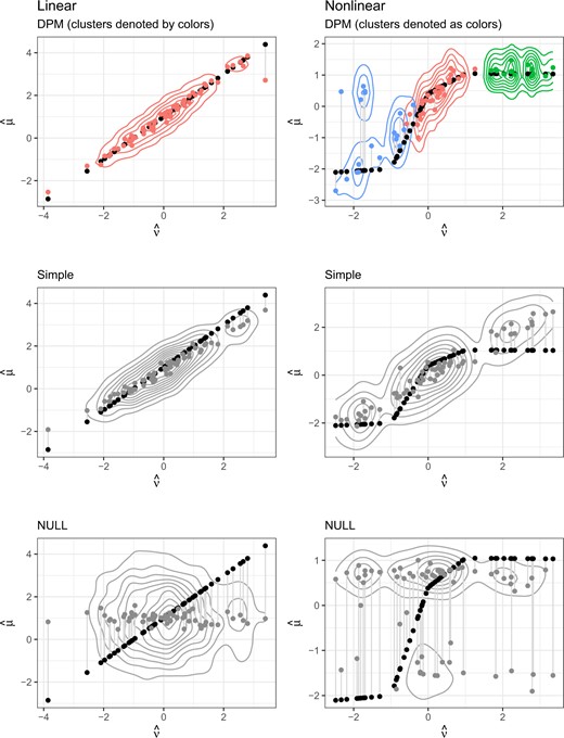
Medians of leave-one-out predictions versus true values, with contours for the posterior density in the linear and nonlinear settings.
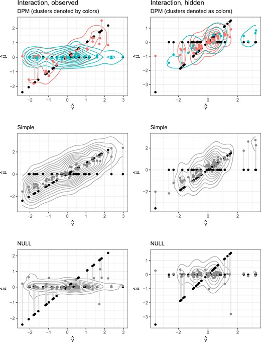
Medians of leave-one-out predictions versus true values, with contours for the posterior density in the two interaction settings.
For the given sample size configuration, our proposed method has difficulty picking up the appropriate cluster in the one and two treatment settings and hence is not able to detect the improved value of the surrogate for the subgroups for which there is surrogate value (Figure S3 of the Supplementary material available at Biostatistics online); however, these are very difficult scenarios. When we consider variation over multiple biomarker groups, as in setting manybiom, we see that the cluster detection improves and we are able to detect the surrogate quality difference (Figure S6 of the Supplementary material available at Biostatistics online). Over the simulation replications in settings 6, 7, and 8, where there are clearly defined clusters, the mean and standard deviation of the proportion of clusters that are correctly identified for each leave-one-out group over the replicates is 0.78 (0.11) in the onetrt setting with |$c_z = c_u = 0$|, 0.80 (0.13) in the onetrt setting with |$c_z = 0.3, c_u = 0$|, 0.48 (0.06) in the twotrt setting with |$c_z = c_u = 0$|, 0.48 (0.06) in the twotrt setting with |$c_z = 0, c_u = 0.3$|, 0.90 (0.05) in the manybiom setting with |$c_z = c_u = 0$|, 0.93 (0.04) in the manybiom setting with |$c_z = 0.3, c_u = 0$|, and 0.94 (0.04) in the manybiom setting with |$c_z = c_u = 0.3$|. Thus, the DPM model is able to identify the correct cluster a large proportion of the time in the setting where there are distinct clusters and enough data.
Additionally, our method is not only able to identify the correct clustering based on surrogate quality that differs by observed subgroups (as in the inter settings) but also when this variation is based on unobserved latent variables (as in the interhide settings)at least in some replicates. Figures S7 and S8 of the Supplementary material available at Biostatistics online show the posterior density of |$\hat{D}$| by clusters (identified using our model), with the different colors indicating different clusters with different surrogate quality. The top panel of Figure S7 of the Supplementary material available at Biostatistics online is for the setting where the clusters are based on a latent variable and the lower panel for the setting where the clusters are based on a biomarker-treatment-level observed covariate. Figure S8 of the Supplementary material available at Biostatistics online shows the settings manybiom (top panel) and twotrt (bottom panel). In these settings, the DPM model is able to detect the differential surrogate value over the clusters.
In summary, the simulation results show that we able to detect and estimate the quality of a surrogate that is useful over all treatments and biomarkers even when the surrogate effect to outcome effect relationship is complex. Our proposed method outperforms the simple model in every case, even when the true data generating mechanism exactly matches the simple parametric model. Additionally, we show our proposed method is able to detect variations in surrogate quality in most settings with adequate power. However, we see that to detect this variation on average we need a large enough subgroup with high surrogate quality, and a large difference in surrogate quality between subgroups (i.e., clearly defined clusters).
4.4. Illustrative example
To illustrate how our proposed methods would be used in practice, from evaluation to the use of the evaluated surrogate in the next setting, we consider a single data set generated under the two treatment (twotrt) setting, with |$c_z = c_u = 0$|, and with independent uniform censoring. Like all of the simulations scenarios, the data generation is based on the code used during the planning phase the Probio trial and fits one of the scenarios that the trial team believed to be plausible.
We assume that both the clinical outcome and surrogate are observed for groups |$1, \ldots, KM = 63$|, and the clinical outcome is not yet observed in the group |$KM+1 = 64$|. Using our model, we would like to predict the unknown treatment effect on the clinical outcome in this group, based on the observed data in the 63 other treatment by biomarker groups in which both the candidate surrogate endpoint and the clinical outcome are observed. To do this, we fit our model using the available data, which does not include the clinical outcome for group |$KM+1 = 64$|, to obtain samples from the posterior of the treatment effect on the clinical outcome for that group. We compute estimates of the prediction error by running the leave-one-out procedure among the remaining 63 groups with complete data.
The results are shown in Figure 3, which plots the posterior estimates of the treatment effects. The target is to predict the treatment effect on the clinical outcome for a new group where the clinical outcome in not measured, indicated by the open circle for the median prediction. This particular effect is correctly assigned to the cluster where there is high surrogate value, and over the iterations the cluster is correctly assigned 97.2|$\%$| of the time.
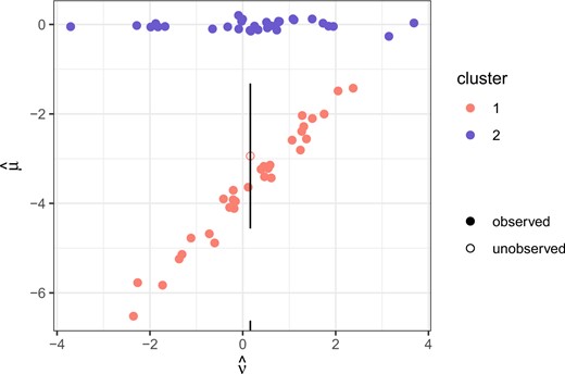
Illustrative example. The filled points represent the posterior medians of the treatment effects with fully observed data, while the unfilled point represents the posterior predicted median for the group where the clinical outcome is unobserved and the vertical line is a prediction interval obtained by adding and subtracting the median leave-one-out error in that cluster.
The overall median prediction error of the DPM model is 1.96, but when looking by cluster, the median error is 2.22 in cluster 2, and 1.63 in cluster 1. In reference to the null model, which has an overall median prediction error of 2.18, the posterior probability of surrogate value |$P(\hat{D} < \hat{D}^0 | \boldsymbol{x}, \boldsymbol{z})$| is 0.47 overall, 0.41 in cluster 2, and 0.54 in cluster 1. It is evident based on these estimates and in the figure that these clusters have differential surrogate value, and the model is able to correctly estimate cluster membership based on the surrogate and group-level covariates alone for the new group.
For future use of the surrogate, one could fit the model with the new treatment effect on the surrogate to determine which cluster the new trial or group gets assigned to, then form posterior predictions of the treatment effect on the clinical outcome as we have done here. It would also be of interest to investigate how the treatment effect on the surrogate and the group level covariates determine cluster membership so that if there are observable determinants of the clustering, those could be used in future (rather than rerunning the full model with the new treatment effect on the surrogate). In this example, the clusters are almost fully identified by two of the treatments. So, one could potentially rerun the model using only these two treatments and then use the resulting model moving forward.
5. Discussion
We propose a flexible and efficient model for assessing the value of a potential surrogate in the context of platform trials. Although the goal of our method is the evaluation of surrogates and the characterization of surrogate heterogeneity in a general platform study, our motivating example is a Bayesian adaptive platform trial with the goal of identifying effective biomarker--treatment combinations in metastatic, castrate-resistant prostate cancer. Our simulation study and illustrative example based on the ProBio trial demonstrates that this method is fit-for-purpose for evaluating the potential surrogate, ctDNA, in that study, but also in general platform studies with or without adaptive randomization or early stopping. The value of ctDNA as a potential surrogate is important to characterize as additional treatment--biomarker combinations are added to the platform study, and also for future trials in earlier-stage prostate cancer, where the time to recurrence or death is much longer. If ctDNA is found to be a high-quality surrogate in a biomarker--treatment combination that is planned for study in early-stage prostate cancer, then the results can potentially be put into clinical practice sooner that they would be without the surrogate. Conversely, evidence that ctDNA is a poor surrogate in that group would be equally valuable to ensure that a treatment is not put into practice on the basis of low quality evidence.
The strengths of the method are the flexibility and data-adaptive nature of the priors in the hierarchical model. In addition the approach allows for baseline group-level covariates to be conditioned on in a flexible manner. To our knowledge, this is a novel approach for surrogate evaluation. Although allowing for inclusion of covariates may make the surrogate quality look poorer, as these covariates may have some predictive ability, if these baseline measures are available this is likely a fairer estimate of the surrogate quality for a surrogate used in practice. Additionally, if surrogate quality varies with these baseline covariates, they allow for better use of the surrogate moving forward.
Due to the clustering in our proposed method, we can assess surrogate quality variation over not only observed subgroups but also data-identified subgroups. The clustering of the DPM is the manner by which it is flexible and data adaptive. More clusters means a more flexible model, and since the number of clusters is data adaptive, our proposed model is as flexible as the data can inform. When distinct clusters are clearly identified by the data, it is worthwhile to explore what those clusters mean and if they indicate differential surrogate value. By its nature, our DPM model allows for such exploration and explanation, something not as straightforward with other types of flexible models, such as splines or locally weighted smoothers. Although simulations show that there are limits to how well this works, particularly when the observed subgroups are very small or the surrogate quality varies only by a latent variable, we are able to detect variations in surrogate quality between large observed subgroups and in some settings with subgroups defined by latent variables. This is an important extension to previous work with the goal of identifying surrogate quality variation (Papanikos and others, 2020) or that allowed for such variation, without evaluating it, in a less flexible manner (Gabriel and others, 2016, 2019).
The shared control arm, adaptive nature of the trial, and stopping rules means that the treatment effect estimates based on the Probio trial may be biased, especially for those that stopped due to superiority or futility (Emerson and Fleming, 1990). Exploration of whether additionally modifications to our method can be made to further reduce bias is an area of future work. Our method specifies a parametric model in the first stage of the hierarchy and a nonparametric model (DPM) at the second stage. Completely nonparametric hierarchical DPM have been developed (Teh and others, 2006). Another avenue for future work would be to implement such mixtures to flexibly model the treatment effects at the first stage of the hierarchy as well. Finally, although we demonstrate how independent censoring can be accounted for, investigation of dependent censoring may be useful for trial settings without registers and whose outcomes do not involve all-cause death.
Software
Software in the form of an R package and complete documentation is available on the corresponding author’s GitHub at https://github.com/sachsmc/dpsurrogate.
Supplementary material
Supplementary material is available online athttp://biostatistics.oxfordjournals.org.
Acknowledgments
Conflict of Interest: None declared.
Funding
Swedish Research Council (2019-00227 to M.C.S.); Swedish Research Council (2017-01898 to E.E.G.); and National Institutes of Health (R01 HL158963 to M.J.D.).
