


Summary
Considerable statistical work done on dynamic treatment regimes (DTRs) is in the frequentist paradigm, but Bayesian methods may have much to offer in this setting as they allow for the appropriate representation and propagation of uncertainty, including at the individual level. In this work, we extend the use of recently developed Bayesian methods for Marginal Structural Models to arrive at inference of DTRs. We do this (i) by linking the observational world with a world in which all patients are randomized to a DTR, thereby allowing for causal inference and then (ii) by maximizing a posterior predictive utility, where the posterior distribution has been obtained from nonparametric prior assumptions on the observational world data-generating process. Our approach relies on Bayesian semiparametric inference, where inference about a finite-dimensional parameter is made all while working within an infinite-dimensional space of distributions. We further study Bayesian inference of DTRs in the double robust setting by using posterior predictive inference and the nonparametric Bayesian bootstrap. The proposed methods allow for uncertainty quantification at the individual level, thereby enabling personalized decision-making. We examine the performance of these methods via simulation and demonstrate their utility by exploring whether to adapt HIV therapy to a measure of patients’ liver health, in order to minimize liver scarring.
1. Introduction
Precision medicine is a research area that seeks to tailor patient care to improve health outcomes, all while reducing over-treatment. For conditions that require sustained therapy through time, assigned treatments may vary through stages of the treatment process. To identify treatment strategies that follow the principles of precision medicine, stage-specific treatments must be allowed to change with patients’ evolving characteristics. These treatment strategies are termed dynamic treatment regimes (DTRs). DTRs contrast static treatment regimes, where time-varying treatments are assigned at the study start. One tool employed to infer about time-varying treatments is marginal structural models (MSMs). These models were developed to evaluate the effect of static regimes (Robins and others, 2000) and later extended to evaluate adherence to DTRs (Murphy and others, 2001), and to identify optimal DTRs (Orellana and others, 2010; van der Laan and Petersen, 2007). MSMs rely on an appealing estimation strategy; they allow scientists to target a finite set of causal estimands without requiring restrictive assumptions about the family of data generating distributions. Semiparametric methods like these have mostly been studied from a frequentist viewpoint.
Semiparametric methods are enviable as they avoid specifying fully parametric probabilistic models that face a high risk of misspecification. These methods may be contrasted with the conventional Bayesian approach to inference, which seeks to multiply a parametric likelihood with a prior. In simple settings, this approach works well, but in more complex settings, like in sequential decision-making, the correct specification of a likelihood is highly suspect. Some work has been done examining the effects of model misspecification in Bayesian inference. For example, Walker (2013) shows that under some conditions, parameters in the misspecified model converge to the minimizers of the Kullback–Leibler divergence. Although this is reassuring, it does mean that inference cannot be guaranteed to be consistent and consequently, treatment recommendations based on misspecified models could be suboptimal. Furthermore, in a setting with time-varying confounding and mediation, the correct specification of a likelihood with parameters representing causal treatment effects will not yield fruitful results; this is because only confounded data are available and these data follow a different probability law. Now, one approach that may guarantee consistency is Bayesian inference via completely nonparametric specifications. In the DTR setting Bayesian nonparametrics have been used to estimate the effect of a small number of dynamic regimes (Xu and others, 2016), but when the family of regimes grows, this approach may not be feasible to identify optimal regimes, due to computational limitations. Generally, it is unresolved how Bayesians may best capitalize on semiparametric approaches to inference about DTRs, and this is one of the challenges that our work addresses.
A variety of other methods for estimating the effect of DTRs have been proposed. For example g-methods including g-computation (Robins, 1986), and g-estimation of structural nested models (Robins, 1993). Other ways by which to identify optimal DTRs include Q-learning (Zhao and others, 2009), and outcome-weighted learning (Zhao and others, 2012). In a Bayesian setting, a standard parametric approach to inference requires specifying the full dynamics of the data generating process in order to learn about dynamic regimes. For example, Saarela and others (2015a) use a predictive Bayesian approach that requires the specification of parametric distributions for outcomes and intermediate covariates in order to identify optimal DTRs. Murray and others (2018) propose a Bayesian adaptation to Q-learning that utilizes machine learning methods for flexible modeling; however, the approach still relies on likelihoods for stage-specific rewards/outcomes. Exceptionally, a few researchers have explored the use of Bayesian nonparametric methods in the DTR setting; Arjas and Saarela (2010) take this approach; however, their method is not computationally feasible as the number of confounders increases.
Ideally, Bayesians would target a finite-dimensional estimand that indexes a large family of regimes, all while working within an infinite-dimensional class of data-generating distributions. Recent work has elucidated ways in which semiparametric inference may be viewed through a Bayesian lens. First, let us review the frequentist setup. Frequentist semiparametrics begins with an estimating function, which under certain modeling assumptions (e.g., for the mean) is an unbiased estimator of zero. For finite samples, setting the estimating function equal to zero and solving for a parameter of interest |$\beta$| yields an estimator |$\hat{\beta}^*_n$| which, under regularity conditions, is consistent and asymptotically normal. A framework for Bayesian semiparametric inference should allow us to take a similar approach. It was not until recently that MSMs for static regimes were provided with a Bayesian motivation by considering the maximization of an expected posterior predictive utility (Saarela and others, 2015b), which required solving for |$\beta$| in a manner analogous to the frequentist procedure. Later, using a similar flavor, Bayesian double robust inference was motivated (Saarela and others, 2016). Other similar recent approaches have further considered inference via utility functions (Bissiri and others, 2016) and through the loss-likelihood bootstrap (Lyddon and others, 2019). What is particularly liberating about these inferential procedures is that Bayesian methods can be used to infer about parameters that are not necessarily embedded in a likelihood, which would undoubtedly be misspecified. However, none of these approaches have examined causal inference for optimal DTRs.
Our work builds on the general framework developed by Saarela and others (2015b) for performing Bayesian causal inference with MSMs. Those authors focused on inferring about stage-specific causal treatment effects of static regimes. As it is well established that MSMs can also be used to infer about (optimal) DTRs, our work seeks to examine how to use this general framework to perform Bayesian causal inference of DTRs. This requires us to carefully interpret the estimands of interest, so that we may conceive of a counterfactual world that allows for causal inference. In the double robust setting, we explore posterior predictive inference for DTRs. This approach to inference was proposed by Saarela and others (2016), but it has only been studied in the cross-sectional setting. We transparently lay out the use of this new framework for Bayesian causal inference, and with this in mind, we explore the performance of this approach via simulations with treatment rules like “assign treatment when a covariate value |$x$| exceeds a threshold |$\theta$|”, with the aim of identifying |$\theta_{\rm opt}$| that optimizes a final outcome. Additionally, with the purpose of illustrating how this methodology may be used in practice, we consider an analysis of HIV therapy using data from the North American AIDS Cohort Collaboration on Research and Design (NA-ACCORD), where we aim to learn about whether to tailor on FIB4, a measure of liver scarring, in order to decide when to switch antiretroviral therapies, with the aim of minimizing long-term liver damage.
In addition to the above-mentioned contributions, we note that frequentist uncertainty quantification does not allow for decision-makers to ask if a new patient will benefit from therapy suggested by an optimal DTR. As we will elaborate, Bayesian posterior predictive inference allows for decision-makers to assess the probability that therapy is optimal for a specific patient, thereby allowing for individualized care. To our knowledge, no other approach quantifies uncertainty at the patient-level decision-making process.
The approach to inference presented here uses the posterior predictive distribution in order to answer causal questions about DTRs; there is no need to model counterfactual outcomes directly. The advantages and detriments of counterfactuals have been studied by, for example, Dawid (2000). Arjas (2012) presents an approach similar to the one taken here, where the quantities of interest are expected conditional outcomes.
2. Estimation strategy
In this section, we first describe the inferential setting and motivate Bayesian inference via a utility maximization framework. We follow this by a precise definition and formulation for connecting two probability laws: the observational world law and the law that allows us to draw causal inference about optimal DTRs by eliminating confounding. We then provide a prior that facilitates robust inference in the developed framework. Lastly, we examine specific utilities that allow for causal inference about optimal DTRs. Some of the developments parallel Saarela and others (2015b) but require some specific considerations for our context; we also take the opportunity to emphasize some of the nuanced arguments present in this framework.
2.1. Inferential setting
We consider a sequential decision problem with |$K$| decision points and a final outcome |$y$| to be observed at stage |$K+1$|. Decisions taken up to stage |$k$| give rise to a sequence of treatments |$\bar{z}_k=(z_1,...,z_k)$|, |$z_j \in \{0,1\}$|. At each stage |$k$|, a set of covariates |$x_k$| is available for decision-making, and it is assumed that these consist of all time-fixed and time-varying confounders. To denote covariate history up to time |$k$|, we write |$\bar{x}_k=\{x_1,...,x_k\}$|. Subscripts are omitted when referencing history through stage |$K$|. We denote a DTR-enforced treatment history by |$g(\bar{x})=(g_1(x_1),...,g_K(\bar{x}_K))$|. Our focus is restricted to deterministic DTRs. Throughout, we will consider a family of DTRs, which will be indexed by |$r \in \mathcal{I}$| to give |$\mathcal{G}=\{g^r(\bar{x});r\in \mathcal{I}\}$|. The index is omitted when it is clear that our focus lies on a single DTR. Treatment and covariate histories may be considered under the probability laws in two worlds: the observational world |$\mathcal{O}$| which denotes the law giving rise to the data in the study population, and the experimental world |$\mathcal{E}$|, which denotes a world in which causal inference may be performed. In the next sections, the definition of |$\mathcal{E}$| will be made more precise. Lastly, variables sampled from a posterior distributions are shown with |$^*$|.
In Appendix A of the Supplementary material available at Biostatistics online, we provide a more general representation in cases where there may be unmeasured causes |$u$| of both intermediary and the final outcome. Outcomes do not inform the treatment assignment mechanism, characterized by a parameter |$\gamma$| (i.e., |$p_{\mathcal{O}}(\gamma|\bar{b}) \propto p(\gamma|\bar{x},\bar{z})$|) (Saarela and others, 2015b). The no unmeasured confounders assumption allows us to model treatment assignment probabilities in (2.1) with observed covariates only as |$p_\mathcal{O}(z_{ij}| \bar{z}_{i(j-1)},\bar{x}_{ij},\gamma_j)$|. This assumption is not often encountered outside the counterfactual framework, so we provide it in Appendix A of the Supplementary material available at Biostatistics online.
2.2. Bayesian MSMs for dynamic regimes
The denominator is the well-known treatment probability in the observational measure; the numerator is the probability of a sequence of treatments conditional on regime assignment. Note that this weight formula differs from that presented in Saarela and others (2015b), though the general procedure is the same. For (2.2) to hold for the entire support of the data, we require that for each |$g$|, |$p_\mathcal{E}(b^*|g,\bar{b})$| be absolutely continuous with respect to |$P_\mathcal{O}$|; this is equivalent to the positivity condition cited in the causal inference literature. Practically, this means that if a patient following regime |$g$| has recorded history |$(\bar{x}_k, \bar{z}_{k-1})$| and receives treatment |$z_k$|, then in the observational world, we should be able to find patients of this sort. Note that as in the frequentist setting, these dynamic MSM weights are not stabilized, and the above argumentation clarifies why the usual stabilization is not possible in the DTR framework. Although importance sampling can motivate inverse probability of treatment weighting (IPW)—a classical approach to estimating MSMs in the frequentist setting—the inferential machinery must still come from semiparametric theory. In Bayesian inference, importance sampling and an appropriate prior lead to a method of inference. In the frequentist literature, the linking of two measures is not usually termed importance sampling; this is done via a Radon–Nykodym derivative. This derivative was first used by Murphy and others (2001) to connect the observational distribution with the distribution in which all patients follow a DTR, and it has been further adapted in works like Johnson and Tsiatis (2004, 2005), Orellana and others (2010), and Hu and others (2018).
Thus, uncertainty in the posterior distribution reflects uncertainty in |$\beta_{\rm opt}$|; this approach to Bayesian inference is discussed by Walker (2010). We may disregard |$C_G$| for the purposes of predictive inference. Modulo Monte Carlo error, this is an exact Bayesian procedure, regardless of the sample size. In work by Saarela and others (2015b), simulations show that multiplying |$\pi_i$| with importance sampling weights dampens the effect of extreme weights thereby leading to improved variance estimators as compared to those relying on asymptotic approximations, the latter tending to underestimate variance. From (2.3), we note that to draw inference in the experimental world, we require an analytic expression for the weight |$w$|; this leads us to modeling the treatment assignment probabilities. We touch on this in Section 2.3. Furthermore, we note that inverse probability weighting methods may not be adequate in settings with many stages, as these require us to take the product of many probabilities, thereby leading to large weights and yielding both bias and imprecision (Robins and others, 2008; Scharfstein and others, 1999). We now present some utilities that allow for causal inference of DTRs.
2.2.1. Utility as negative squared error loss:
We see that the |$\beta_n$| which maximizes the equation above is the same as that which solves the estimating equation in Orellana and others (2010). Indeed, we see why our approach may be regarded as a way to unify Bayesian inference with dynamic MSMs. Now, we need not limit ourselves to a finite family of regimes. If the family of DTRs is indexed by a continuous parameter, then a relaxed positivity condition described in Orellana and others (2010) will allow us to perform inference on values of the index where positivity may not hold. This condition says that instead of requiring that we observe patients who followed all regimes of interest, we require for patients to follow a subset of regimes. More specifically, |$\beta$| in |$h(\beta,r)$| may be identified |$\forall r\in \mathcal{I}$| even when the positivity assumption fails for some |$r$|, and it suffices to observe |$r$| for sufficient points such that |$\beta$| is identifiable. For example, a model |$h(\beta,r)=\beta_0+\beta_1r + \beta_2r^2$| that is correctly specified is identifiable if positivity is met for at least three values of |$r\in \mathcal{I}$|. Of course, the model should be correct in the range of inference. For example, if the identified optimal |$r$| is far from the range of observed values, we should question the resulting inference. When searching for optimal DTRs via smooth modeling, we must keep in mind that we seek two optimal posteriors: the first is the posterior distribution of |$\bar{\beta}=(\beta_{0,{\rm opt}},\beta_{1,{\rm opt}},\beta_{2,{\rm opt}})$|; the second is the posterior distribution of |$r_{\rm opt}$| which is a deterministic function of |$\bar{\beta}$|.
Fitting procedure for Bayesian dynamic MSM.
2.2.2. Utility as negative log likelihood:
Note that |$w^*_{\mathcal{A}_i} \sum_{r\in \mathcal{A}_i} \ell(y_i|g^{r},\beta)$| is a weighted likelihood; in accordance with the weighted likelihood bootstrap, |$\beta_{\rm opt}(\pi)$| may be regarded as a sample from the posterior distribution of |$\beta$| under a flat prior. Thus, repeated sampling from this posterior allows for quantification of uncertainty around |$\beta$|. Other priors may be incorporated via sampling importance resampling, but this is not essential and is not the focus of our work.
2.3. Implementation
Then, for every draw of |$\Pi$|, we first fit the weighted treatment propensity model and use the resulting weight |$w(\pi)$| in (2.4). By computing |$E_\Pi\{E_\mathcal{E}[U(b^{*},g,\beta)|\bar{b},\Pi]\}$|, we are indirectly incorporating the uncertainty about |$\gamma_j$| into the estimation procedure.
3. Predictive double robust Bayesian inference for DTRs
These are expected outcomes in the observational world, conditional on subjects who had covariate history |$\bar{x}_{k}$| and that followed the regime |$g$| up to time |$k$|. It can be shown via a conditional expectation argument that |$E_g[y^*|\bar{b}]=E_\mathcal{O}[\phi^*_2(x^*_1)|\bar{b}]$|, the estimand of interest.
Next, we describe how models for |$\phi_k^*$| may be fit in a Bayesian framework; following this, we motivate the double robust estimator when models for |$\phi^*_{k+1}$| are correct or when models for |$w^*_k$| are correct. Based on the de Finetti representation in (2.2), we see that outcome models are parameterized by |$\tau$| such that |$\phi^*_{k+1}(\bar{x}_k)=\phi^*_{k+1}(\bar{x}_k;\tau)$|. From (3.7) and (3.8), we see exactly how a model should be fit for the mean of the conditional outcomes. We should begin by fitting a model for time point |$k=K$| and continue backward; the outcomes for stage |$k$| can be computed once a model for stage |$k+1$| has been fit. We can treat uncertainty in |$\tau$| analogously to how we treated uncertainty in |$\gamma$|, the parameter corresponding to the treatment assignment model in the observational world: we make it dependent on |$\Pi$| via a nonparametric, noninformative prior. However, instead of posing a likelihood model as was done for the treatment assignment mechanism, we consider the negative squared error loss utility and posit a model for the conditional outcomes. Then, for every draw of |$\Pi$|, we can estimate |$\phi^*_{k+1}(\bar{x}_k,\pi)=E_g[y^*| \bar{x}_k^*=\bar{x}_k, \pi, \tau(\pi)]$|. In Appendix C.1 of the Supplementary material available at Biostatistics online, we provide details as to how |$\tau$| may be estimated and incorporated into the inferential procedure.
Models for the |$\phi$|s and |$w$|s now depend on |$\Pi$| and may be incorporated into the inferential process as in (2.3). Furthermore, we may compute |$E_g[y^*| \bar{b}]=E_\Pi\left[E_g[y^*| \bar{b}, \Pi]\right]$| by resampling Dirichlet weights, thereby enabling us to obtain a double robust estimator for the value of a DTR, including its uncertainty. As mentioned, the double robust Bayesian estimator proposed is only for the marginal mean of a DTR, not for the parameters in a model for the marginal mean linking a family of DTRs (e.g., |$E[y^*|\bar{b},g^r]=\beta_0+\beta_1r+ \beta_{2} r^{2}$|). In order to obtain double robust estimators of the latter, an appropriate utility would have to be proposed so that when importance sampling is used to link the experimental world with the observational world, the obtained expression in the observational world is doubly robust. Then, to use the proposed estimator to identify optimal DTRs, we are required to perform a grid search. Murphy and others (2001) suggested that outcome models should be coherently parameterized so that for |$k_2>k_1$|, a model conditional on information up to time |$k_2$| would yield a model conditional on information up to time |$k_1$| when covariates between |$k_2$| and |$k_1$| are marginalized.
4. Individualized decision-making
Now that we have developed the inferential approach, we turn our attention to examining how to incorporate this into an individualized decision-making scheme. This consideration is particular to the DTR setting that we explore. For illustrative purposes, we focus on the following class of regimes: treat if |$x_k>\theta$| for |$k=1,...,K$|. Suppose that a new patient is observed with covariate value |$x_1^{\rm new}$|. Our interest is in deciding whether this patient should be treated based on our belief about the optimal |$\theta$|. To do this, we are interested in computing |$P(\theta^*_{\rm opt}<x_1^{\rm new}|\bar{b})$|. This may be done by taking a sample of size |$m$| from the posterior distribution and computing |$p_1=(1/m) \sum_\theta {\rm 1}\kern-0.24em{\rm I}(\theta_i^*<x_1^{\rm new})$|. Indeed this can be done for all stages |$p_k$|. Effectively, this probability is informing the decision-maker about how certain they should be in switching treatment given the patient’s current health status, if the aim is to select an optimal therapy. It is then up to the decision-maker to make a treatment decision given that probability. Note that a patient’s decision about treatment at a given stage does not alter the optimality of consequent decision rules, though it may alter the optimality of the overall treatment course. This individualized approach may be taken with any optimal regime derived through the proposed methodology, and we elaborate on this in the simulations.
5. Simulations
In this section, we use simulations to evaluate how this Bayesian approach to inference can be used to infer about optimal DTRs. We focus on multistage problems with a sample size of |$n=500$|. All results are presented over 500 Monte Carlo replications. For comparison, we also provide results for the frequentist approach. Generally the strategy was to induce time varying confounding with treatment-confounder feedback. All intermediary variables were Gaussian, and all treatment variables Bernoulli. We followed the approach in Stephens (2016) to generate outcomes that allowed for the analytic identification of the optimal regimes. The true value (expected outcome) under the optimal regime was obtained by generating a large sample of data in which patients adhered to the optimal regime. Further simulation details can be found in Appendix D of the Supplementary material available at Biostatistics online, as well as results for other sample sizes and for when intermediary variables are Gamma-distributed.
For simulation I, we considered a family of regimes indexed by |$\theta_1,\theta_2$| where treatment is assigned when |$x_k$| exceeds |$\theta_k$|, |$\theta_k \in [0,1]$|, |$k=1,2$|. The known optimum is |$(\theta_{1{\rm opt}}, \theta_{2{\rm opt}})=(0.4, 0.8)$| and the outcome |$y=x_1- (-\theta_{1{\rm opt}}+x_1)({\rm 1}\kern-0.24em{\rm I}_{\theta_{1{\rm opt}}>z_1}-z_1) - (-\theta_{2{\rm opt}}+x_2)({\rm 1}\kern-0.24em{\rm I}_{\theta_{2{\rm opt}}>z_2}-z_2) + \sqrt{0.5}\epsilon$|, |$\epsilon \sim N(0,1)$|. We evaluate the performance of both the IPW and double robust estimator thereby leading us to compute these estimators for discrete values of |$\theta_k \in \left\{0,0.1,0.2,...,0.9,1\right\}$|. Table 1 shows the results of the estimation procedure. The first column indicates the type of estimation procedure that was used. The second refers to the model specification. For the double robust estimator “None” means that both treatment and outcome models are miss-specified ; “Treat” means the treatment models are correctly specified; “Outcome” means that outcome models are correctly specified; “Both” means all models are correctly specified. “IPW” refers to the IPW estimator with correctly specified treatment models. For incorrectly specified models, we use intercept-only regressions. For the Bayesian approach, point estimates are provided at the posterior mean. For simulation I, the mean outcome at the optimal regime can be seen (from the data-generating mechanism) to be 0.
Results for simulation I (|$n$|=500; 500 Monte Carlo replicates). Point estimates are means across Monte Carlo replicates; standard deviations are Monte Carlo standard deviations.
| Method | Model correct | Posterior mean of |$\hat{\theta}_{1opt}$| | Posterior mean of |$\hat{\theta}_{2opt}$| | Estimated outcome train Pop. | Coverage probability |$\theta_{1opt},\theta_{2opt}$| | Mean outcome test Pop. |
|---|---|---|---|---|---|---|
| Frequentist | None | 0.247 (0.116) | 0.641 (0.183) | 0.250 (0.120) | — | 0.587 (0.012) |
| Frequentist | Treat | 0.468 (0.232) | 0.753 (0.207) | 0.045 (0.066) | — | 0.584 (0.017) |
| Frequentist | Outcome | 0.385 (0.193) | 0.735 (0.210) | 0.022 (0.065) | — | 0.588 (0.014) |
| Frequentist | Both | 0.415 (0.182) | 0.793 (0.162) | 0.018 (0.056) | — | 0.591 (0.011) |
| Frequentist | IPW | 0.441 (0.205) | 0.747 (0.209) | 0.035 (0.064) | — | 0.587 (0.014) |
| Bayesian | None | 0.246 (0.124) | 0.641 (0.192) | 0.271 (0.119) | 0.860, 0.914 | 0.586 (0.012) |
| Bayesian | Treat | 0.480 (0.253) | 0.759 (0.203) | 0.070 (0.064) | 0.990, 0.964 | 0.582 (0.019) |
| Bayesian | Outcome | 0.371 (0.207) | 0.737 (0.232) | 0.037 (0.065) | 0.974, 0.986 | 0.585 (0.015) |
| Bayesian | Both | 0.414 (0.194) | 0.797 (0.166) | 0.029 (0.056) | 0.978, 0.974 | 0.590 (0.012) |
| Bayesian | IPW | 0.454 (0.218) | 0.761 (0.214) | 0.055 (0.063) | 0.990, 0.964 | 0.585 (0.017) |
In Table 1, we observe that estimators with at least one set of models correct are unbiased. As expected, when the treatment and outcome models are all correctly specified, efficiency is maximized. The coverage probability measures the proportion of time that the true optimum is inside a 95|$\%$| credible interval, across replications. As far as we are aware, there is no way to obtain a confidence interval for the optimal threshold in the frequentist setup. This is because we have evaluated the estimator in a grid of thresholds |$\theta$| and identified the |$\hat{\theta}_{\rm opt}$| that maximizes the mean outcome; for the Bayesian setup, we have sampled the posterior distribution of |$\theta_{\rm opt}$|. “Estimated Outcome Train Pop.” refers to estimated expected outcome under the optimal regime, this is known to be 0; “Mean Outcome Test Pop.” refers to the mean outcome under the optimal DTR, in a new population with a different distribution for intermediate covariates. Thinking about the mean outcome in a test population allows us to contemplate how the identified optimal DTR will perform once deployed in the real world. We see that the frequentist and Bayesian methods perform similarly, and surprisingly the “no models correct” scenario leads to good performance in the testing set, though this is due in part to the scale of the value function which has a narrow range (see Appendix D of the Supplementary material available at Biostatistics online). The uncertainty measures for |$\theta_{k,{\rm opt}}$| appear to be slightly higher for the Bayesian analysis than for the frequentist analysis. One reason for this may be that the Bayesian method acknowledges uncertainty in the outcome and treatment models, whereas the frequentist method takes these as known. The coverage probability for |$\theta_1$| in the no models correct scenario is low, and surprisingly it is close to nominal for |$\theta_2$|. For the other setups, the coverage probabilities are slightly higher than their nominal value. Of course, it is important to keep in mind that this was a discrete problem and the coverage probabilities depend on the coarseness of the exploration grid; we have observed in other simulations that finer grids lead to further tightening of the confidence intervals toward the nominal value (results not shown). However, this must be balanced with the computational costs of an estimation procedure on a fine grid.
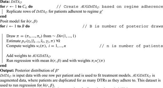
Now, we can ask whether newly observed patients will benefit from the estimated optimal rule. For illustration, we restrict the family of regimes to have a common threshold across periods: |$\theta_{1}=\theta_{2}=\theta$|, with |$\theta_{\rm opt}=0.6$| (see Appendix D of the Supplementary material available at Biostatistics online). Figure 1(a) shows the probability that a patient should receive treatment |$z=1$| at stage 1 for a single Monte Carlo replicate. This is a step function as |$\theta$| was computed over a set of discrete values. Patients with low and high values of |$x_1$| experience high certainty as to whether they should receive optimal treatment or not. Patients whose covariate is near the true optimal threshold of 0.6 experience low certainty. Figure 1(b) shows the same result across 500 Monte Carlo replicates, emphasizing that there is high uncertainty around the true value. It can also be useful to obtain a smooth decision curve. This may be done by evaluating the double robust estimator over a much finer grid of points or by modeling |$E[y^*|\bar{b},g^{\theta}]$| via a smooth function such as |$\beta_0+\beta_1\theta+\beta_2 \theta^2$| (quadratic) and using IPW. Figure 1(c) shows the results of the individualized rule with the quadratic model and IPW estimator; the decision rule is much smoother and provides high certainty for most values of |$x_1$|, except for those closest to 0.6. Figure 1(d) shows the Monte Carlo variation around this curve; most uncertainty is around the true value of the threshold.
Simulation I, stage 1 individualized treatment probabilities: (a) Individualized decision rule using double robust estimator with only the treatment model correct; (b) Same as (a) over 500 Monte Carlo replicates; (c) Individualized decision rule using IPW with a quadratic MSM; (d) Same as (c) over 500 Monte Carlo replicates.
For simulation II, we explore a family of regimes indexed by |$\psi_1,\psi_2,\psi_3$| such that |$\psi_{1}x_{k1}+\psi_{2}x_{k2}>0.5-3\psi_3u; k=1,...,4$|; |$x_{k1}, x_{k2}$| are normally distributed intermediary covariates and |$u$| is a binary baseline covariate. This regime has an interpretation that treatment should be given if the weighted sum of |$x_{k1}$| and |$x_{k2}$| is above a threshold, and this threshold depends on patients’ baseline covariate |$u$|. Increments of |$0.05$| were used for |$\psi_1,\psi_2$| and of |$0.1$| for |$\psi_3$|. Appendix D.3 of the Supplementary material available at Biostatistics online shows the data generating mechanism for this setup. The optimal regime is given by |$\psi_{1 opt}=\psi_{2 opt}=0.5, \psi_{3 opt}=0.1$|, with a value of |$1$|. We see from Table 2 that all scenarios, except the no models correct scenario are unbiased, with the all models correct scenario yielding the best results. Correctly specifying the outcome model provides improvement in the estimation of the value at the optimum over just getting the treatment model correct. We do not include a |$\psi_2$| column in the table, as the constraint |$\psi_1+\psi_2=1$| makes this redundant. We note again that the coverage probabilities are high, recall that this is driven by the coarseness of the exploration grid; a finer grid in this problem would be very computationally intensive. Appendix D.2 of the Supplementary material available at Biostatistics online presents a similar simulation without the binary covariate.
Results for simulation II (|$n$| = 500; 500 Monte Carlo replicates). Point estimates are means across Monte Carlo replicates; standard deviations are Monte Carlo standard deviations.
| Method | Model correct | Posterior mean of |$\hat{\psi}_{1opt}$| | Posterior mean of |$\hat{\psi}_{3opt}$| | Estimated outcome train Pop. | Coverage probability |$\psi_{1opt}, \psi_{2opt}$| | Mean outcome test Pop. |
|---|---|---|---|---|---|---|
| Freq. | None | 0.590 (0.126) | 0.103 (0.104) | 2.003 (0.355) | — | 0.526 (0.064) |
| Freq. | Treat | 0.479 (0.157) | 0.101 (0.125) | 1.160 (0.155) | — | 0.530 (0.057) |
| Freq. | Outcome | 0.503 (0.048) | 0.102 (0.020) | 1.004 (0.068) | — | 0.581 (0.010) |
| Freq. | Both | 0.499 (0.031) | 0.100 (0.004) | 1.000 (0.065) | — | 0.585 (0.004) |
| Freq. | IPW | 0.464 (0.157) | 0.089 (0.134) | 1.198 (0.184) | — | 0.529 (0.055) |
| Bayes. | None | 0.589 (0.123) | 0.094 (0.106) | 2.200 (0.351) | 0.952 0.996 | 0.549 (0.022) |
| Bayes. | Treat | 0.481 (0.165) | 0.089 (0.124) | 1.254 (0.150) | 0.992 1 | 0.539 (0.025) |
| Bayes. | Outcome | 0.498 (0.050) | 0.101 (0.016) | 1.008 (0.066) | 0.994 1 | 0.587 (0.005) |
| Bayes. | Both | 0.497 (0.029) | 0.100 (0.004) | 1.001 (0.064) | 1 1 | 0.591 (0.003) |
| Bayes. | IPW | 0.468 (0.163) | 0.072 (0.130) | 1.317 (0.198) | 0.992 1 | 0.537 (0.024) |
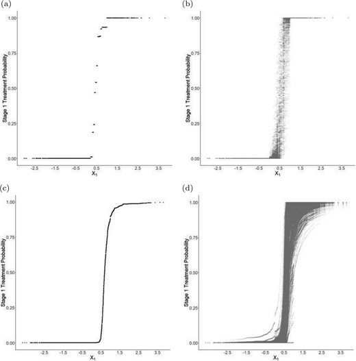
In Figure 2, we further illustrate how the Bayesian framework can be leveraged for individualized inference. We observe, for one replicate, the probability that a patient should be treated under the optimal decision rule, given as set of covariates. These probabilities are computed by using the posterior distribution of |$\psi_{1{\rm opt}}, \psi_{2{\rm opt}}, \psi_{3{\rm opt}}$| via |$P(\psi_{1{\rm opt}}^*x_{11}+\psi_{2{\rm opt}}^*x_{12}+\psi_{3{\rm opt}}^*u>0.5)$|. There are regions of high certainty that indicate patients should or should not receive treatment according to the optimal rule; there are also regions with more uncertainty regarding the choice of optimal treatment. In fact, patients with baseline covariate |$u=0$| face higher uncertainty overall than those with |$u=1$|.
Simulation II individualized treatment probabilities using IPW estimator; (a) Stage 1 treatment probability for those with |$u=0$| (b) Stage 1 treatment probability for those with |$u=1$|.
There is some debate in the literature on choice of double versus singly robust estimators; see e.g. Kang and Schafer (2007) and Bang and Robins (2005). Our simulations emphasize that a lot is to be gained, in precision and accuracy, if we correctly specify the outcome models, when compared to the double robust estimator with only treatment models correct or the IPW estimator. Efficiency is maximized when all models are correct, thereby clarifying that these considerations are not just theoretical; they also impact analyses with finite sample size. When deciding whether to use the singly robust or the doubly robust estimator, it is important to ask what is better understood: the treatment assignment process, or the outcome process.
6. Case study: analysis of the NA-ACCORD
Treatment for HIV infection with antiretroviral therapy (ART) must be lifelong to maintain control of HIV viral replication and improve immune function. Consequently, there is concern that some combinations of drugs may cause long-term harm. The multidrug nature of this therapy allows for some flexibility in treatment course. Research by Klein and others (2016) is consistent with the possibility that some ART agents contribute to long-term liver damage in patients with chronic hepatitis C (HCV) infection. ART agents, like protease inhibitors (PI), may also help reduce adverse liver outcomes by providing virologic control (Macías and others, 2006), while also having some detrimental effects on liver health (Young and others, 2021). We examine how to tailor ART therapy to reduce liver damage by exploring the use of Bayesian dynamic MSMs for tailoring therapy to patients’ FIB4 score, an age-adjusted score that quantifies liver fibrosis; higher values indicate greater damage (Sterling and others, 2006). We aim to identify whether there is an optimal FIB4 score at which patients should switch therapy, in order to minimize subsequent FIB4. In particular, for the purposes of demonstrating the use of the proposed methods, we explore the effect of switching into PI (|$z=1$|) and away from any other ART regimen (|$z=0$|) when FIB4 score surpasses a level |$\theta$|, and when all patients start out on a non-PI based therapy. This is a thresholding regime, where we search for the optimal |$\theta$| in the DTR: switch when FIB4 |$>\theta$|.
We use data from the NA-ACCORD to identify a cohort of patients who initiated ART therapy from 2004 onwards, the period in which modern ART treatments were approved. Patients in this cohort may or may not have other viral infections, such as HCV and hepatitis B (HBV). Study initiation (time zero) is the first instance of ART treatment, after which patients are followed-up for a 12-month exposure ascertainment period. It is in this period where we may examine which DTRs patients follow. Lastly, outcomes are taken to be the first FIB4 measurement 18–30 months after study initiation. The outcome observation period is as defined because liver measurements are not taken at every follow-up visit, though they should occur at least annually as per standard of care. Patients are lost to follow-up if they stopped receiving ART, had missing ART records, or if they did not have an observed outcome. The range of thresholds is determined by the 5th and 95th quantile of FIB4 scores at baseline. We identify patient records every 6 months and record the treatment that patients received. Potential confounders included were: time-varying CD4-cell count, time-varying viral load, and the following baseline variables: insurance status, indicator of risky alcohol consumption, drug use, HCV status, HBV status, race, and sex.
Based on the 6-month observation intervals, there were a total three decision points, each requiring a set of models. Potential confounders were identified a priori through discussions with a subject matter expert. Stage-specific propensity scores were then fit to achieve balance across treatments at each time point. Censoring weights were incorporated to eliminate selection bias. For the doubly robust estimator, it was assumed that the variables in outcome models explained both confounding and/or selection. The models that were fit can be found in Appendix E of the Supplementary material available at Biostatistics online. Sensitivity analyses were performed in order to determine whether results were sensitive to model specifications. Balance from the propensity scores was assessed using standardized differences and by using a frequentist fit of the propensity scores. Balance was examined at all stages. Outcome models were examined to ensure the predicted distribution did not differ from the observed.
For a fixed value of |$\theta$|, patients are indicated to switch treatments when their FIB4 measurements surpass |$\theta$|. Accordingly, patients in the study could be categorized into five groups for each regime (|$g^\theta$|) considered: those (1) indicated to switch but did not switch (ISNS), or switched at the wrong time; (2) indicated to switch and switched (ISS); (3) not indicated to switch and did not switch (NISNS); (4) not indicated to switch and switched (NISS); and (5) those who were assigned to PI at baseline (NR). Patients indicated to switch were given six months to do so (a grace period). To improve the properties of the estimators, we normalized the weights in the analysis and assessed positivity for each candidate regime by checking whether the distribution of the propensity scores at each interval for the modeled treatment are similar in the regime adherent group and the regime nonadherent group. The propensity to switch treatment was generally small, highlighting that relatively few individuals contribute to the estimation of our regime of interest — a limitation that must be acknowledged; more details can be found in Appendices E.3 and E.4 of the Supplementary material available at Biostatistics online. Only patients in the ISS and NISNS groups could adhere to a regime for the full study period. Consequently, patients in the other groups were artificially censored when they deviated off the specified regime. 95|$\%$| credible intervals were calculated for all point estimates, approximated using 500 draws from the posterior distribution; point estimates were reported at the posterior mean. Details of the analysis plan can be found in Appendix E of the Supplementary material available at Biostatistics online.
We evaluated the estimators at thresholds of 0.4 to 2.8 in units of 0.2; the minimum and maximum threshold value correspond to the 5th and 95th percentile of the FIB4 distribution. In Table 3, we present follow-up information for a subset of these regimes. We did not posit a marginal structural model as a function of |$\theta$| (e.g. a quadratic form) as we wanted to make use of both the IPW and double robust estimators. Although our overall sample size is large, we see that only half of patients follow a non-PI ART regimen at study start. Additionally, roughly 30|$\%$| of ISS and NISS patients are censored or artificially censored. The number of NISNS patients varies strikingly across regimes. However, this is to be expected: for a threshold of 0.5, only a small proportion of patients are not indicated to switch, and a relatively large proportion of patients switch in the first year of the study. The sample size in the ISS group is generally low, which is unfortunate. In part, this is due to the fact that when patients are indicated to switch, not only should they switch, but they should switch within the indicated time. The sample size in the ISS group is further reduced for large values of |$\theta$| as for these values, only a small number of patients would be indicated to switch.
NA-ACCORD case study: follow-up information for a subset of regimes (|$n$|=22,768)
| |$\theta$| | ISNS | ISS | NISNS | NISS | NR | Uncensored ISS | Uncensored NISNS |
|---|---|---|---|---|---|---|---|
| 0.4 | 12172 | 611 | 244 | 8 | 9733 | 412 | 244 |
| 1.0 | 6798 | 398 | 5618 | 221 | 9733 | 276 | 5618 |
| 1.6 | 3194 | 213 | 9222 | 406 | 9733 | 143 | 9222 |
| 2.2 | 1732 | 143 | 10684 | 476 | 9733 | 89 | 10684 |
| 2.8 | 1136 | 111 | 11280 | 508 | 9733 | 73 | 11280 |
ISNS = Indicated to switch & did not switch; ISS = Indicated to switch & switched; NISNS = Not indicated to switch & did not switch; NISS = Not indicated to switch and switched; NR =Received PI at baseline.
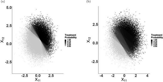
From Figure 3(a), we confirm that we are underpowered to detect any differences in final FIB4 scores, and that the doubly robust estimator provided some gains in efficiency. It is noteworthy that FIB4 scores drop overall at the end of the study, compared to the baseline values. We note that from this figure, there is no interior point that clearly minimizes FIB4 score, thereby suggesting that there is no benefit to tailoring. A threshold of |$\theta=0.4$| yields a DTR that is very close to the static treatment always switch into PI. Though this may raise the question as to why patients would be given a drug other than PI, we remind the reader that there are a variety of other ART treatments, some of which may be more beneficial and some which may be more detrimental. From Table 4, we can examine the expected outcomes for a subset of regimes. We note that the IPW and doubly robust estimator yield very similar point estimates across most regimes; both estimators point to the same conclusions. In addition, Figure 3(a) also leads us to question the utility of individualized inference in this scenario. Though the figure shows a relatively flat relationship between the value function and the threshold (with considerable uncertainty), the value function under adherence to each candidate regime is not flat, as is shown in Figure S4 of the Supplementary material available at Biostatistics online. Consequently, we can ask the probability that a patient’s FIB4 value is greater than the optimal threshold. This results in Figure 3(b), which indicates that when a patient’s FIB4 score is at 0.8 or greater, they have a high probability of being above the optimal threshold. We discuss this further in Appendix E.6 of the Supplementary material available at Biostatistics online.
(a) Mean FIB4 score under each DTR based on Bayesian IPW and doubly robust analyses, with 95|$\%$| credible intervals (from 500 posterior draws). (b) Individualized treatment probability using double robust estimator. Note that in (a) the points corresponding to each method are presented out of phase for illustrative purposes. In reality, points are on top of each other starting at 0.4 and continuing in increments of 0.2.
NA-ACCORD case study: expected FIB4 (outcome) under adherence to regime |$\theta$|. Numbers in brackets are posterior standard deviations.
| |$\theta$| | IPW | Double robust |
|---|---|---|
| 0.4 | 1.145 (0.054) | 1.116 (0.048) |
| 1.0 | 1.176 (0.051) | 1.133 (0.044) |
| 1.6 | 1.205 (0.048) | 1.159 (0.039) |
| 2.2 | 1.221 (0.048) | 1.183 (0.040) |
| 2.8 | 1.214 (0.045) | 1.184 (0.039) |
| |$\theta$| | IPW | Double robust |
|---|---|---|
| 0.4 | 1.145 (0.054) | 1.116 (0.048) |
| 1.0 | 1.176 (0.051) | 1.133 (0.044) |
| 1.6 | 1.205 (0.048) | 1.159 (0.039) |
| 2.2 | 1.221 (0.048) | 1.183 (0.040) |
| 2.8 | 1.214 (0.045) | 1.184 (0.039) |
This analysis had several limitations. First, the follow-up may have been too short for the outcome of interest, as switching therapies may not have an immediate effect on liver scarring; this is likely a long-term process. The reason for the short follow-up was that after the first year, therapeutic switches were relatively rare. Also, there was a trade-off in extending the follow-up time: it would allow for more therapeutic switches but also increase artificial censoring due to going off regime. Though many confounders were included in the analysis, some may have been missed. Importantly, we did not have information on why patients switched therapy. Additionally, it would have been beneficial to study only patients coinfected with HCV and HBV, as these are at higher risk of liver complications. However, sample size limitations did not allow for this.
7. Discussion
In this work, we explored recently developed Bayesian semiparametric methods to infer about optimal DTRs. For this purpose, we sought to transparently develop a way to utilize Bayesian dynamic MSMs, this involved targeting experimental world causal parameters when only observational world data was available. We also inferred about optimal DTRs via posterior predictive inference and a double robust estimator; this approach had not been studied in a longitudinal DTR setting. Our simulations showed that the proposed methods work well, though they exhibit slightly more variability than their frequentist counterpart. The analysis of the NA-ACCORD provided a demonstration of how these methods might be used in clinical research, though we note that the results were limited by the fact that therapeutic switching was infrequent in practice. Still, this case study aimed to show that our proposed inference could be implemented meaningfully. Though our approach does not necessitate counterfactual notation, the idea of counterfactuals still permeates this work; the experimental world considered is indeed a world where, counter to fact, patients have been randomized to a specific treatment strategy of interest. Additionally, the resulting conditional posterior predictive quantities are equal to their counterfactual counterparts in this unconfounded world. Throughout, we focused on the nonparametric Bayesian bootstrap in order to draw inference in a noninformative, robust way. Indeed our choice of prior allowed us to connect our approach to the way frequentist semiparametric estimators are obtained. Though these methods may feel different, they have the same ingredients that appear in conventional Bayesian analyses. A prior leads to posterior inference in the observational world, and importance sampling allows us to infer about worlds that are of scientific interest. When we are interested about inferring about parameters in a utility, the Dirichlet process prior that we make use of implicitly induces a prior on these parameters; these ideas as explored further in Stephens and others (2021). We remind the reader that the proposed method is valid for any sample size. We also note that methods discussed herein are not limited to decisions taken at fixed dates; they may also be triggered by events. For example, a second-line therapy may be given only when first-line therapy lacks efficacy, as in Krakow and others (2017).
8. Software
Software in the form of R code can be found on GitHub on the following link: https://github.com/Danroduq/Semi-parametric-Bayesian-DTRs.
Supplementary material
Supplementary material is available online at http://biostatistics.oxfordjournals.org.
Acknowledgments
The authors are grateful to the NA-ACCORD, and the full acknowledgment can be found in the Appendix of the Supplementary material available at Biostatistics online. The content of this manuscript is solely the responsibility of the authors.
Conflict of Interest: None declared.
Funding
A doctoral fellowship from Natural Sciences and Engineering Research Council of Canada (NSERC) to D.R.D.; Discovery Grants from NSERC to E.E.M.M. and D.A.S.; a career award from the Fonds de recherche du Québec - Santé and a Canada Research Chair (CRC) in Statistical Methods for Precision Medicine to E.E.M.M.; a CRC Tier I and reports grants for investigator-initiated studies from ViiV Healthcare, Merck, and Gilead; and consulting fees from ViiV Healthcare, Merck, AbbVie, and Gilead to M.B.K.
