


Summary
Validation of phenotyping models using Electronic Health Records (EHRs) data conventionally requires gold-standard case and control labels. The labeling process requires clinical experts to retrospectively review patients’ medical charts, therefore is labor intensive and time consuming. For some disease conditions, it is prohibitive to identify the gold-standard controls because routine clinical assessments are performed for selective patients who are deemed to possibly have the condition. To build a model for phenotyping patients in EHRs, the most readily accessible data are often for a cohort consisting of a set of gold-standard cases and a large number of unlabeled patients. Hereby, we propose methods for assessing model calibration and discrimination using such “positive-only” EHR data that does not require gold-standard controls, provided that the labeled cases are representative of all cases. For model calibration, we propose a novel statistic that aggregates differences between model-free and model-based estimated numbers of cases across risk subgroups, which asymptotically follows a Chi-squared distribution. We additionally demonstrate that the calibration slope can also be estimated using such “positive-only” data. We propose consistent estimators for discrimination measures and derive their large sample properties. We demonstrate performances of the proposed methods through extensive simulation studies and apply them to Penn Medicine EHRs to validate two preliminary models for predicting the risk of primary aldosteronism.
1. Introduction
Many efforts have been spent on the development of automated phenotyping algorithms using electronic health record (EHR) data, which are classification rules based on features extracted from patients’ EHRs, both structured and unstructured, to infer whether a patient has a specific phenotype (Shivade and others, 2013;Pathak and others, 2013;Hong and others, 2019;Yu and others, 2016). Discrimination and calibration are the two main aspects for validating phenotyping algorithms. Discrimination is the ability of separating patients with from without the specific phenotype. Commonly used metrics include true positive rate (TPR), false positive rate (FPR), positive predictive value (PPV), negative predictive value (NPV), and area under the ROC curve (AUC) (Claesen and others, 2015). Probability estimates could be unreliable even when the phenotyping algorithms have good discrimination, for example, they can be systematically higher or lower. The agreement between observed and predicted phenotype probabilities are called calibration. Model calibration is especially important when the actual probability of a patient having the phenotype is needed in downstream inference (Hong and others, 2019;Wang and others, 2020).
Conventionally, the development and validation of EHR-based phenotyping algorithms rely on a curated data set, in which every patient is labeled accurately with regard to presence (case) or absence (control) of the phenotype of interest. For example, conventional Hosmer–Lemeshow type of calibration tests are based on the differences between observed and expected numbers of cases across patient subgroups (Hosmer Jr and others, 2013;Hosmer and others, 1988;Tsiatis, 1980;Windmeijer, 1990;Song and others, 2014). Accurate assignment of case and control labels usually requires domain experts to retrospectively review patients’ medical charts, therefore is labor intensive and time consuming. This limits the achievable sample size and compromises phenotyping accuracy. In addition, for many diseases, since patients are usually actively screened based on clinical suspicion, the EHR data are often insufficient for identifying a large group of gold-standard controls. Therefore, frequently, most readily accessible EHR data is for an incomplete set of gold-standard cases and a large number of unlabeled patients whose case and control status are unknown (Elkan and Noto, 2008). Hereafter, we refer to the data for such an incompletely labeled EHR cohort as “positive-only” data.
We previously proposed a maximum likelihood approach to developing phenotyping models using positive-only data within an anchor variable framework (Zhang and others, 2019). This approach greatly reduces dependency on gold-standard labeling since it does not require labeled controls. It relies on the specification of an anchor variable (Halpern and others, 2014) for the target phenotype to label the set of cases instead of labor-intensive manual chart reviewing. An anchor variable is a binary variable specified by domain experts as highly informative of patients’ true phenotype status. The patients with positive anchor variable values form a random subset of all cases in the population because of two unique properties of the anchor variable. First, an anchor variable has perfect positive predictive value, i.e., anchor being positive indicates the presence of the phenotype, while it being negative is nondeterministic of the patient’s phenotype status. Second, anchor variable has constant sensitivity, i.e., conditional on phenotype presence, the anchor being positive or negative is independent of phenotyping model predictors. For example, a pathologic diagnosis of cancer in most scenarios can serve as a positive anchor because of its high PPV and imperfect sensitivity due to variability in practice or documentation, variability in diagnostic categories, or data incompleteness (Zhang and others, 2019). Domain knowledge and a small set of chart reviews are typically exploited for anchor variable specification and validation (Halpern and others, 2014;Halpern and others, 2016); however, it typically requires less upfront effort from clinical experts as compared to labor-intensive chart review for identifying gold-standard cases and controls.
In this project, motivated by avoiding labor intensive labeling, we propose statistical methods for validating phenotyping models using positive-only EHR data within an anchor variable framework. To overcome the challenge caused by the absence of gold-standard labels for the unlabeled patients, we first propose a model-free estimator for the number of cases in each risk subgroup among the unlabeled patients, taking advantage of the two defining characteristics of the anchor variable. The model-free and model-based (i.e., “expected”) estimated numbers of cases are expected to be close when the phenotyping model is well calibrated. Therefore, the extent to which these two estimates disagree reflects the level of poor calibration of the phenotyping model. We then construct a novel calibration statistic quantifying the disagreement across risk subgroups of the unlabeled patients. We also demonstrate how to estimate the calibration slope using positive-only data with our previously proposed maximum likelihood approach (Zhang and others, 2019).
In organizing the article, we first present our statistic for assessing model calibration using positive-only data when phenotype prevalence is known or unknown respectively. We also derive the asymptotic distribution of the proposed statistic and show that it follows a |$\chi^2$| distribution when the fitted model is well calibrated. We then show how to estimate the calibration slope using positive-only data. We next present estimates of discrimination performance measures including TPR, FPR, PPV, NPV, and AUC, and show their asymptotic properties. We conduct extensive simulation studies to assess the type I error rate of the proposed calibration statistic, demonstrate its power for detecting poor calibration, as well as to assess statistical consistency of the proposed estimators for discrimination performance measures. Lastly, we apply the proposed validation methods to assess calibration and discrimination performances of the preliminary phenotyping models for primary aldosteronism that were derived from Penn Medicine EHR data (Zhang and others, 2019).
2. Methods
2.1. The anchor variable framework
2.2. Model calibration using positive-only EHR
Note that although the expression |$P({\bf X};\widehat{\boldsymbol{\beta}})$| appears in the expression (2.3), it does not have to be a true prediction model in order to yield a valid statistic |$\widehat p^n \{Y=1|P({\bf X};\boldsymbol{\beta}) \in I_l, S=0\}$|. It is only used as a way to group the covariates. In fact, we could have chosen a completely arbitrary function to group the covariates, the statistic will still be valid. However, this is not the case in the construction of |$\widehat p^m\{Y=1|P({\bf X};\widehat{\boldsymbol{\beta}}) \in I_l, S=0\}$|, which will not be a consistent estimator of |$p\{Y=1|P({\bf X};\boldsymbol{\beta}) \in I_l, S=0\}$| if the prediction model |$P({\bf X};\boldsymbol{\beta})$| is wrong. In this sense, we name the two estimators nonparametric and parametric respectively.
2.2.1. When |$q$| is known
2.2.2. When |$q$| is unknown
Strictly speaking, the nonparametric estimator |$\widehat p^n \{Y=1|P({\bf X};\widehat{\boldsymbol{\beta}}) \in I_l, S=0\}$| is not totally nonparametric when we replace the instance of |$q$| using |$N^{-1}\sum_{i=1}^N P({\bf X}_i;\widehat{\boldsymbol{\beta}})$|, in the sense that when the prediction model |$P({\bf X};\boldsymbol{\beta})$| is wrong, |$\widehat p^n \{Y=1|P({\bf X};\widehat{\boldsymbol{\beta}}) \in I_l, S=0\}$| is no longer a consistent estimator of |$ p\{Y=1|P({\bf X};\boldsymbol{\beta}) \in I_l, S=0\}$|. Fortunately, we are only interested in the deviation between the parametric and nonparametric statistics, and they continue to be valid estimators of the same quantity under |$H_0$| and deviate under alternative.
We emphasize that how the risk subgroups |$I_l$|, |$l=1,2, \ldots, K$|, are formed does not affect the development and validity of the proposed calibration methods. In the following, we form the risk subgroups according to the fitted probabilities |$P({\bf X};\widehat {\boldsymbol{\beta}})$| in such a manner that the use of |$K=10$| risk subgroups results in cutpoints defined at the values |$k/10, k=1,2,...,9$|, and the risk subgroups contain all patients with fitted probability between the adjacent cutpoints, e.g., the first group contains patients with |$P({\bf X}; \widehat{\boldsymbol{\beta}})\leqslant0.1$|, the second group contains patients with |$0.1 < P({\bf X}; \widehat{\boldsymbol{\beta}}) \leqslant 0.2$|, |$\dots$|, and the tenth group contains those with |$0.9<P({\bf X};\widehat{\boldsymbol{\beta}})\leqslant1$|.
2.2.3. Estimation of calibration slope using positive-only EHR
2.3. Discrimination performance assessment among positive-only EHR
Similar estimates of PPV|$_v$|, NPV|$_v$|, and AUC and their respective asymptotic properties are provided in Appendix D.
3. Simulations
3.1. Simulation settings
We conducted extensive simulation studies to evaluate the validity and feasibility of the proposed Chi-squared statistics |$T^{q}$| and |$T^{nq}$| for model calibration among unlabeled patients, and reported their type I error rate and power at 0.05 nominal significance level. We also evaluated the consistency and efficiency of the proposed estimators for discrimination measures using positive-only data.
The regression coefficients were set at |$(\beta_1,\beta_2,\beta_3)=(0.2,0.4,0.6)$|, |$(\beta_4,\beta_5,\beta_6)=(-1.0,-1.4,1.8)$|, |$(\beta_7,\beta_8,\beta_9)=(-2.0,2.4,2.8)$|, with |$(X_1,X_2,X_3)$|, |$(X_4,X_5,X_6),$| and |$(X_7,X_8,X_9)$| resembling weak, moderate, and strong predictors, respectively. The intercept parameter was selected in such a way that the phenotype prevalence was fixed at |$20\%$|. We fixed the anchor sensitivity |$c$| at 0.5, and generated the anchor variable |$S$| as follows: (i) when |$Y=1$|, |$S$| takes the value |$1$| with probability |$c$| and (ii) when |$Y=0$|, |$S$| is always |$0$|. For each Monte Carlo simulation, we ran 1000 replicates for each set-up.
3.2. Simulation results
As shown in Table 1, when the fitted model is correctly specified, the nonparametric and parametric estimates of cases were nearly identical across all risk groups, with difference |$\leq$|1, indicating good calibration. The quantile plots of the statistics |$T^{q}$| and |$T^{nq}$| suggest that the distributions of the proposed statistics were well approximated by |$\chi^2$| distributions with degrees of freedom |$K$| or |$K-1$| when |$q$| is known or unknown respectively (Figures 1 and 2). As shown in Table 3, the type I error rates for both |$T^{q}$| and |$T^{nq}$| were very close to the 0.05 nominal level, independent of the number of subgroups |$K$|.
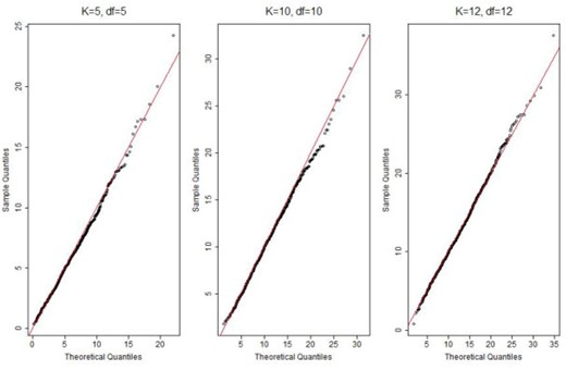
QQ plot of the calibration statistic |$T^{q}$| with |$K=5, 10, 12$| and |$N=50\,000$|. “df”: degree of freedom.
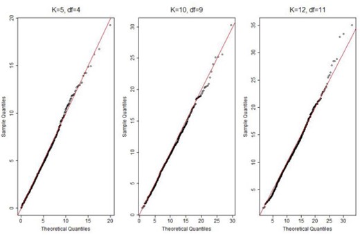
QQ plot of the calibration statistic |$T^{nq}$| with |$K=5, 10, 12$| and |$N=50\,000$|. “df”: degree of freedom.
Contingency table of nonparametric vs. parametric estimates of number of cases in intervals of estimated probabilities. Sample size |$N=50,000$|. Estimates are averaged over 1000 replications. “Correct”: fitted model correctly specified; “Minor”: fitted model missing weak predictors |$(X_1, X_2, X_3)$|; “Moderate”: fitted model missing moderate predictors |$(X_4, X_5, X_6)$|; “Severe”: fitted model missing weak and moderate predictors |$(X_1 -X_6)$|; “Npara”: nonparametric; “Para”: parametric.
| Correct | Minor | Moderate | Severe | ||||||||
|---|---|---|---|---|---|---|---|---|---|---|---|
| Interval | Npara | Para | Npara | Para | Npara | Para | Npara | Para | |||
| 0.0_0.1 | 98 | 98 | 122 | 124 | 326 | 335 | 338 | 348 | |||
| 0.1_0.2 | 100 | 100 | 133 | 126 | 391 | 365 | 413 | 385 | |||
| 0.2_0.3 | 108 | 109 | 140 | 135 | 391 | 375 | 411 | 396 | |||
| 0.3_0.4 | 121 | 120 | 151 | 149 | 395 | 392 | 415 | 411 | |||
| 0.4_0.5 | 138 | 137 | 168 | 169 | 410 | 417 | 428 | 435 | |||
| 0.5_0.6 | 162 | 162 | 194 | 198 | 438 | 454 | 453 | 470 | |||
| 0.6_0.7 | 200 | 200 | 238 | 244 | 483 | 507 | 496 | 522 | |||
| 0.7_0.8 | 268 | 268 | 314 | 323 | 562 | 589 | 572 | 600 | |||
| 0.8_0.9 | 427 | 427 | 492 | 503 | 723 | 739 | 721 | 736 | |||
| 0.9_1.0 | 3483 | 3483 | 3198 | 3178 | 1331 | 1278 | 1239 | 1185 | |||
Type I error rates of the proposed calibration tests when we partition the estimated probabilities into |$K=5,10,12$| groups at different sample sizes.
| |$K=$| | 5 | 10 | 12 | |
|---|---|---|---|---|
| |$T^{q}$| | |$N=30 000$| | 0.045 | 0.046 | 0.042 |
| |$N=50 000$| | 0.042 | 0.047 | 0.045 | |
| |$N=80 000$| | 0.042 | 0.049 | 0.039 | |
| |$T^{nq}$| | |$N=30 000$| | 0.041 | 0.048 | 0.045 |
| |$N=50 000$| | 0.049 | 0.046 | 0.049 | |
| |$N=80 000$| | 0.048 | 0.048 | 0.049 |
To evaluate the performance in terms of power, we deliberately fitted three misspecified models by omitting some predictors out of the model in order to demonstrate different levels of calibration: minor, which omitted weak predictors |$(X_1,X_2,X_3)$|; moderate, which omitted moderate predictors |$(X_4,X_5,X_6)$|; severe, which omitted both the weak and moderate predictors (|$X_1$| through |$X_6$|) from the model in (3.1). Note that poor calibration can be caused by many different reasons, we hereby use these three misspecified models as simple illustration examples. As shown in the calibration plots (Figure 3), contingency table (Table 1) and calibration table (Table 2), the minor misspecified model is not poorly calibrated, while poor calibration is demonstrated in the moderate and severe misspecified models. The level of disagreement between nonparametrically and parametrically estimated number of cases, i.e., indication of poor calibration, increased as the misspecification became more severe. Take probability interval 0.9–1.0 as an example, the difference between the nonparametric and parametric estimates of the number of cases increased from 20 to 53 and 54 respectively. The results in Table 4 also suggest that the fitted models weren’t poorly calibrated when only weak predictors were left out, with power less than 0.24 even when the sample size |$N$| was increased to 80 000. When moderate predictors were left out, our proposed calibration tests were able to flag the poor calibration. For example, at |$K=10$| and |$N=50\,000$|, the power was 0.69 and 0.73 when |$q$| is known, and was 0.59 and 0.63 when |$q$| is unknown, when moderate, or both weak and moderate predictors failed to be included in the fitted model respectively. The power also improved when the sample size increased as we expected. For example, when both weak and moderate predictors were missing from the model, at |$K=10$|, the power increased from 0.46 to 0.92 as the sample size increased from 30 000 to 80 000 when |$q$| was known, and increased from 0.38 to 0.87 when |$q$| was unknown (Table 4). As expected, knowing the phenotype prevalence |$q$| also helped increase power of the calibration test. For example, the power for detecting severe misspecification increased from 0.87 to 0.92 when |$N=80\,000$| and |$K=10$|. As illustrated in Table 4, the power of the proposed calibration tests |$T^q$| and |$T^{nq}$| did not rely much on the selection of the number of subgroups |$K$|, as the observed power was very similar across different |$K$| values, |$5, 10,$| and |$12$|. As shown in Table S1 of the Supplementary material available at Biostatistics online, the calibration slopes estimated using positive-only data were very close to their respective benchmarks, which were calculated using fully observed |$Y$|, regardless of whether the fitted model was correct or misspecified.
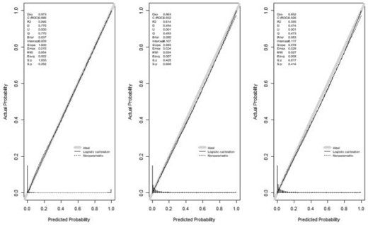
Calibration plot of the three mis-specified models (from left to right: minor, moderate, severe) with |$N=50\,000$|.
Calibration results for the fitted models with |$K=10$| and |$N=50,000$|. “Correct”: fitted model correctly specified; “Minor”: fitted model missing weak predictors |$(X_1, X_2, X_3)$|; “Moderate”: fitted model missing moderate predictors |$(X_4, X_5, X_6)$|; “Severe”: fitted model missing weak and moderate predictors |$(X_1 -X_6)$|. |$T^{q}$| and |$T^{nq}$| are averaged over 1000 replications; p-value is calculated based on the averaged statistics |$T^{q}$| and |$T^{nq}$|.
| Correct | Minor | Moderate | Severe | ||||||||
|---|---|---|---|---|---|---|---|---|---|---|---|
| |$T^{q}$| | |$p$|-value | |$T^{q}$| | |$p$|-value | |$T^{q}$| | |$p$|-value | |$T^{q}$| | |$p$|-value | ||||
| When |$q$| is known | 9.66 | 0.47 | 12.12 | 0.28 | 23.28 | 0.01 | 23.99 | 0.01 | |||
| When |$q$| is unknown | 8.64 | 0.47 | 10.88 | 0.28 | 19.56 | 0.02 | 20.21 | 0.02 | |||
Power of the proposed calibration test for detecting model misspecification at different numbers of subgroups |$K$| and sample size |$N$|. For model misspecification: “Minor”: fitted model missing weak predictors |$(X_1,X_2,X_3)$|; “Moderate”: fitted model missing moderate predictors |$(X_4,X_5,X_6)$|; “Severe”: fitted model missing weak and moderate predictors |$(X_1 - X_6)$|.
| Minor | Moderate | Severe | ||||||||||
|---|---|---|---|---|---|---|---|---|---|---|---|---|
| |$K=$| | 5 | 10 | 12 | 5 | 10 | 12 | 5 | 10 | 12 | |||
| |$T^{q}$| | |$N=30 000$| | 0.10 | 0.09 | 0.10 | 0.46 | 0.43 | 0.43 | 0.47 | 0.46 | 0.44 | ||
| |$N=50 000$| | 0.14 | 0.12 | 0.11 | 0.70 | 0.69 | 0.68 | 0.73 | 0.73 | 0.71 | |||
| |$N=80 000$| | 0.20 | 0.17 | 0.16 | 0.91 | 0.92 | 0.91 | 0.93 | 0.92 | 0.92 | |||
| |$T^{nq}$| | |$N=30 000$| | 0.10 | 0.09 | 0.08 | 0.36 | 0.33 | 0.30 | 0.38 | 0.38 | 0.33 | ||
| |$N=50 000$| | 0.14 | 0.12 | 0.12 | 0.58 | 0.59 | 0.57 | 0.64 | 0.63 | 0.63 | |||
| |$N=80 000$| | 0.24 | 0.20 | 0.19 | 0.81 | 0.85 | 0.84 | 0.85 | 0.87 | 0.87 | |||
To evaluate consistency of the proposed estimators for discrimination performance measures based on positive-only data, we compared these estimates to their benchmarks, which were calculated using the true phenotype status. As shown in Table 5, when the data-generating model (3.1) was fitted to each simulated data set, the accuracy measure estimators, |$\widehat{{\rm TPR}_v}$|, |$\widehat{{\rm FPR}_v}$|, |$\widehat{{\rm PPV}_v}$|, |$\widehat{{\rm NPV}_v}$|, and |$\widehat{\rm AUC}$| were very close to their respective benchmarks. The negligibly small biases indicated statistical consistency of the proposed estimators. To assess the asymptotic variance as an approximation of the true variance, we compared the average asymptotic (ASE) and empirical (ESE) standard errors based on 1000 replications. Some differences were observed with |$N=10\,000$| as shown in Table S2 of the Supplementary material available at Biostatistics online. However the differences became negligible when the sample size was increased to 80 000 (Table S2 of the Supplementary material available at Biostatistics online). It appears that relatively large sample sizes are needed for the asymptotic variances to approximate closely to the true variances. We therefore recommend using bootstrapping to estimate standard errors in practice.
Discrimination performance measures evaluated among unlabeled patients when true phenotype status is observed or with positive-only data for |$N=10 000$| and |$N=80 000$|. Results are based on the mean over 1000 replications.
| |$Y$| observed (Benchmark) | Positive-only | |||||||||||
|---|---|---|---|---|---|---|---|---|---|---|---|---|
| Cutoff | PPV | NPV | TPR | FPR | AUC | |$\widehat{\rm PPV}$| | |$\widehat{\rm NPV}$| | |$\widehat{\rm TPR}$| | |$\widehat{\rm FPR}$| | |$\widehat{\rm AUC}$| | ||
| |$N=10 000$| | 0.2 | 0.677 | 0.994 | 0.959 | 0.059 | 0.990 | 0.678 | 0.995 | 0.962 | 0.059 | 0.991 | |
| 0.4 | 0.789 | 0.989 | 0.913 | 0.032 | — | 0.792 | 0.989 | 0.918 | 0.031 | — | ||
| 0.6 | 0.868 | 0.981 | 0.855 | 0.017 | — | 0.873 | 0.982 | 0.860 | 0.016 | — | ||
| 0.8 | 0.935 | 0.971 | 0.766 | 0.007 | — | 0.939 | 0.971 | 0.769 | 0.006 | — | ||
| |$N=80 000$| | 0.2 | 0.675 | 0.995 | 0.961 | 0.059 | 0.990 | 0.675 | 0.995 | 0.961 | 0.059 | 0.990 | |
| 0.4 | 0.789 | 0.989 | 0.916 | 0.032 | — | 0.789 | 0.989 | 0.916 | 0.031 | — | ||
| 0.6 | 0.870 | 0.982 | 0.857 | 0.016 | — | 0.871 | 0.982 | 0.858 | 0.016 | — | ||
| 0.8 | 0.938 | 0.971 | 0.765 | 0.007 | — | 0.938 | 0.971 | 0.766 | 0.006 | — | ||
4. Data example
4.1. Preliminary phenotyping models for primary aldosteronism
Primary aldosteronism (PA) is the most common cause of secondary hypertension, accounting for 5-10|$\%$| of hypertensive patients (Rossi and others, 1996;Oenolle and others, 1993;Shigematsu and others, 1997). PA is severely under-detected (Mulatero and others, 2016). In order to efficiently identify patients with PA from Penn Medicine EHR for further research, we have previously developed two PA phenotyping models (Zhang and others, 2019). To do this, we first specified two anchor variables for PA, |$S_1$| and |$S_2$|. |$S_1$| was specified as whether the patient was included in an existing expert-curated PA research registry. Every patient included in this registry is a definitive PA case (Wachtel and others, 2016), because they underwent a diagnostic procedure, adrenal vein sampling, which was only performed on patients who were confirmed to have primary aldosteronism. |$S_2$| was specified by adding patients with laboratory test orders for adrenal vein sampling cortisol or aldosterone testing, which is only performed as part of the adrenal vein sampling procedure, to |$S_1$|-positive set.
The data set contained 6319 patients who had orders for a PA screening laboratory test, with 149 (2.4|$\%$|) cases labeled by |$S_1$| and 196 (3.1|$\%$|) labeled by |$S_2$|. For each anchor |$S_1$| and |$S_2$|, we developed a corresponding logistic regression phenotyping model in the form of (2.2) with predictors including demographics, laboratory results, encounter metadata, diagnosis codes, selected variables that were available at the time of screening and some variables extracted from unstructured clinical text. The detailed forms of the phenotyping models are included in Supplementary Tables 6 and 7 of Zhang and others (2019). The labeling sensitivity of |$S_1$| and |$S_2$| was estimated as 0.56 (95|$\%$| CI 0.46–0.65) and 0.61 (95|$\%$| CI 0.54–0.69), and PA prevalence as 4|$\%$| (95|$\%$| CI 3|$\%$|–5|$\%$|) and 5|$\%$| (95|$\%$| CI 4|$\%$|–6|$\%$|), respectively. In this study, we assess the calibration and discrimination performance of the developed models among the unlabeled patients.
4.2. Validation of PA phenotyping models
To validate the two positive-only EHR phenotyping models for PA, we tested their calibration and evaluated their discrimination performances among the unlabeled patients. All results are based one 1000 bootstrap replicates. As shown in Table 6, we observed good agreement between the nonparametric and parametric estimates of PA cases for both anchors, with difference |$\leq$|3 for all intervals except for 0.9–1.0, which had 106 nonparametric vs. 99 parametric PA cases when using anchor |$S_1$|. As shown in Table 7, when the PA prevalence was unknown, the calibration statistic |$T^{nq}$| achieved p-values of 0.78 (|$T^{nq}$| = 5.60) and 0.53 (|$T^{nq}$| = 8.05) for |$S_1$| and |$S_2$| based models when the number of subgroups |$K$| was taken to be 10, indicating good calibration. The PA prevalence in our patient population is around |$5\%$| based on historical information. We therefore applied the calibration test |$T^{q}$|, which indicated excellent goodness-of-fit of the fitted models (|$T^{q}=5.84$| and |$5.42$|; p-value |$=0.83$| and |$0.86$| for |$S_1$| and |$S_2$| based models, respectively). We then evaluated their discrimination performance using the proposed estimators. For both anchors, the model achieved |$AUC>0.98$|. The PPV and TPR were estimated as |$0.83$| and |$0.75$| at the decision threshold 0.5 for |$S_1$|-based phenotyping model, and |$0.81$| and |$0.79$| for |$S_2$|-based model (Table 8). Charts for patients with |$p(Y=1|{\bf X};\widehat{\boldsymbol\beta})>0.5$| were reviewed by clinicians. According to the chart review results, the PPVs for models based on |$S_1$| and |$S_2$| were estimated at |$0.78$| and |$0.77,$| respectively. Interestingly, the estimated PPVs based on the |$S_1$| model were slightly higher than those based on the |$S_2$| model, while the estimated TPRs were slightly lower. This might be due to the lower prevalence of PA cases among the patients unlabeled with |$S_2$|. The standard errors based on the |$S_2$| model were generally smaller for the corresponding estimates. This is reasonable because |$S_2$| labeled more cases.
Contingency table of nonparametric vs. parametric estimates of PA cases in intervals of estimated probabilities for the two PA phenotyping models based on anchor variable |$S_1$| and |$S_2$|, respectively.
| Anchor |$S_1$| | Anchor |$S_2$| | ||||
|---|---|---|---|---|---|
| Interval | Npara | Para | Npara | Para | |
| 0_0.1 | 12 | 11 | 7 | 7 | |
| 0.1_0.2 | 8 | 6 | 4 | 4 | |
| 0.2_0.3 | 3 | 6 | 6 | 3 | |
| 0.3_0.4 | 7 | 5 | 1 | 3 | |
| 0.4_0.5 | 7 | 6 | 5 | 3 | |
| 0.5_0.6 | 8 | 9 | 3 | 5 | |
| 0.6_0.7 | 0 | 5 | 3 | 3 | |
| 0.7_0.8 | 8 | 10 | 5 | 5 | |
| 0.8_0.9 | 10 | 13 | 6 | 7 | |
| 0.9_1 | 106 | 99 | 85 | 84 | |
Calibration results for PA phenotyping models built upon two anchors when |$q$| is assumed known as |$5\%$| or unknown respectively when the number of subgroups |$K$| was taken to be 10.
| Anchor |$S_1$| | Anchor |$S_2$| | ||||
|---|---|---|---|---|---|
| |$T^{q}$| | p-value | |$T^{q}$| | p-value | ||
| When |$q$| is known | 5.84 | 0.83 | 5.42 | 0.86 | |
| When |$q$| is unknown | 5.60 | 0.78 | 8.05 | 0.53 | |
| Anchor |$S_1$| | Anchor |$S_2$| | ||||
|---|---|---|---|---|---|
| |$T^{q}$| | p-value | |$T^{q}$| | p-value | ||
| When |$q$| is known | 5.84 | 0.83 | 5.42 | 0.86 | |
| When |$q$| is unknown | 5.60 | 0.78 | 8.05 | 0.53 | |
Estimated accuracy measures and their associated empirical standard errors (in parentheses) for identifying PA patients using our proposed method for positive-only data. Results based on mean over 1000 bootstrap replicates.
| Anchor |$S_1$| | Anchor |$S_2$| | ||||||||||
|---|---|---|---|---|---|---|---|---|---|---|---|
| cutoff | |$\widehat{\rm PPV}$| | |$\widehat{\rm NPV}$| | |$\widehat{\rm TPR}$| | |$\widehat{\rm FPR}$| | |$\widehat{\rm AUC}$| | |$\widehat{\rm PPV}$| | |$\widehat{\rm NPV}$| | |$\widehat{\rm TPR}$| | |$\widehat{\rm FPR}$| | |$\widehat{\rm AUC}$| | |
| 0.1 | 0.413 | 0.997 | 0.89 | 0.03 | 0.983 | 0.395 | 0.998 | 0.906 | 0.028 | 0.986 | |
| (0.124) | (0.001) | (0.041) | (0.005) | (0.008) | (0.072) | (0.001) | (0.025) | (0.004) | (0.005) | ||
| 0.2 | 0.559 | 0.997 | 0.85 | 0.016 | — | 0.533 | 0.997 | 0.872 | 0.015 | — | |
| (0.128) | (0.001) | (0.054) | (0.003) | — | (0.077) | (0.001) | (0.03) | (0.002) | — | ||
| 0.3 | 0.666 | 0.996 | 0.815 | 0.009 | — | 0.639 | 0.997 | 0.844 | 0.01 | — | |
| (0.122) | (0.001) | (0.064) | (0.002) | — | (0.074) | (0.001) | (0.034) | (0.002) | — | ||
| 0.4 | 0.755 | 0.995 | 0.782 | 0.006 | — | 0.732 | 0.996 | 0.817 | 0.006 | — | |
| (0.11) | (0.001) | (0.071) | (0.001) | — | (0.071) | (0.001) | (0.039) | (0.001) | — | ||
| 0.5 | 0.828 | 0.994 | 0.748 | 0.003 | — | 0.81 | 0.996 | 0.787 | 0.004 | — | |
| (0.093) | (0.002) | (0.078) | (0.001) | — | (0.063) | (0.001) | (0.042) | (0.001) | — | ||
| 0.6 | 0.882 | 0.993 | 0.707 | 0.002 | — | 0.871 | 0.995 | 0.753 | 0.002 | — | |
| (0.078) | (0.002) | (0.087) | (0.001) | — | (0.056) | (0.001) | (0.048) | (0.001) | — | ||
| 0.7 | 0.915 | 0.992 | 0.66 | 0.001 | — | 0.906 | 0.994 | 0.708 | 0.001 | — | |
| (0.065) | (0.002) | (0.098) | (0.001) | — | (0.052) | (0.001) | (0.054) | (0.001) | — | ||
| 0.8 | 0.922 | 0.991 | 0.601 | 0.001 | — | 0.919 | 0.993 | 0.649 | 0.001 | — | |
| (0.058) | (0.002) | (0.107) | (0.001) | — | (0.047) | (0.001) | (0.06) | (0.001) | — | ||
| 0.9 | 0.899 | 0.989 | 0.518 | 0.001 | — | 0.915 | 0.991 | 0.571 | 0.001 | — | |
| (0.068) | (0.003) | (0.12) | (0.001) | — | (0.053) | (0.002) | (0.066) | (0.001) | — | ||
5. Discussion
Traditional methods for model validation depend on a fully labeled validation set. Our proposed methods pave the way to greatly alleviate the need for labor intensive manual labeling, because they do not require labeled controls and rely on the specification of an anchor variable to label the set of cases in positive-only data. Collectively, the anchor variable framework offers a highly efficient approach to EHR phenotyping as well as a cost effective data resource for model validation. As anchor variables continue to be developed for a wide variety of phenotypes, we expect that the methods for model validation proposed here, together with the maximum likelihood approach for model development proposed previously (Zhang and others, 2019), will not only advance accurate EHR phenotyping algorithm development but also facilitate their generalizability, since a well-chosen anchor variable may be more easily transferred across institutions.
Reasons for poor calibration can be complicated in real-life problems. In this work, we omitted predictors from data generation models to induce ill-calibrated models. We intended to use the current simulation studies to demonstrate the validity of our proposed test statistic regarding its size and power. Our results showed that the test statistic is reasonably sensitive to the degree of ill-calibration. More complicated settings, such as plasmode simulations leveraging existing data set can be further studied in future research.
Unlike the Hosmer–Lemeshow test whose result depends markedly on the number of risk subgroups, our proposed calibration tests are robust to the number of subgroups because our proposed calibration statistic |$T^q$| or |$T^{nq}$| follow a |$\chi^2$| distribution as long as the variance-covariance matrix |${\bf V}_K$| or |${\bf V}_{K-1}$| is well approximated. Thus sparse cells should be avoided in |${\bf U}_{K}$| or |${\bf U}_{K-1}$| and we proposed grouping based on fixed values. In initial attempts of grouping based on percentiles of fitted probabilities, we observed that the expected number of cases can be very low in the lower percentile intervals, especially when the phenotype prevalence is low. This could lead to empty cells in |${\bf U}_{K}$| or |${\bf U}_{K-1}$|, compromising the estimation of |${\bf V}_K$| or |${\bf V}_{K-1}$| so as to sabotage the performance of the proposed calibration tests. We recommend that the within-group expected number of cases be taken into consideration in the selection of the number of subgroups |$K$|. Similar to the Hosmer–Lemeshow goodness-of-fit test, the power of our proposed calibration test can be low when the sample size is not large. In such situation, we recommend looking at the contingency table instead of relying on the p-value of the calibration test. As shown in Table 1, poor calibration can be revealed by the disagreement between the nonparametric and parametric estimates of the number of cases.
The proposed calibration statistics asymptotically follow the |$\chi^2$| distribution when the fitted model is correctly specified provided that the anchor variable is well defined, i.e., the anchor variable has perfect PPV and constant sensitivity. Thus with a validated anchor variable, small p-values of the proposed calibration tests mean that the model is a poor fit. Noting that the calibration results can be affected by either model misspecification or invalid anchor variable specification, further research is needed for extensions to discriminate the two causes.
6. Software
Software in the form of R code, together with a sample input dataset and complete documentation is available at "https://github.com/zhanglingjiao/Calibration-paper or upon request from the corresponding authors ([email protected] or [email protected]).
7. Supplementary material
Supplementary material is available online at http://biostatistics.oxfordjournals.org.
8. Acknowledgments
Conflict of Interest: None declared.
