


Summary
Three-dimensional (3D) genome spatial organization is critical for numerous cellular processes, including transcription, while certain conformation-driven structural alterations are frequently oncogenic. Genome architecture had been notoriously difficult to elucidate, but the advent of the suite of chromatin conformation capture assays, notably Hi-C, has transformed understanding of chromatin structure and provided downstream biological insights. Although many findings have flowed from direct analysis of the pairwise proximity data produced by these assays, there is added value in generating corresponding 3D reconstructions deriving from superposing genomic features on the reconstruction. Accordingly, many methods for inferring 3D architecture from proximity data have been advanced. However, none of these approaches exploit the fact that single chromosome solutions constitute a one-dimensional (1D) curve in 3D. Rather, this aspect has either been addressed by imposition of constraints, which is both computationally burdensome and cell type specific, or ignored with contiguity imposed after the fact. Here, we target finding a 1D curve by extending principal curve methodology to the metric scaling problem. We illustrate how this approach yields a sequence of candidate solutions, indexed by an underlying smoothness or degrees-of-freedom parameter, and propose methods for selection from this sequence. We apply the methodology to Hi-C data obtained on IMR90 cells and so are positioned to evaluate reconstruction accuracy by referencing orthogonal imaging data. The results indicate the utility and reproducibility of our principal curve approach in the face of underlying structural variation.
1. Introduction
The three-dimensional (3D) configuration of chromosomes within the eukaryote nucleus is important for several cellular functions, including gene expression regulation, and has also been linked to translocation events and cancer driving gene fusions (Mitelman and others, 2007). While direct visualization of 3D architecture has improved (see Section 2.9), imaging challenges pertaining to chromatin compaction and dynamics persist. However, the ability to infer chromatin architectures at increasing resolution has been enabled by chromosome conformation capture (3C) assays (Dekker and others, 2002). In particular, when coupled with next generation sequencing, such Hi-C methods (Lieberman-Aiden and others, 2009; Duan and others, 2010) yield an inventory of pairwise, genome-wide chromatin interactions, or contacts. In turn, the contact data form the basis for reconstructing 3D configurations (Zhang and others, 2013; Varoquaux and others, 2014; Ay and others, 2014; Zou and others, 2016; Rieber and Mahony, 2017). While many novel conformational-related findings have flowed from direct analysis of contact level data, added value of performing downstream analysis based on attendant 3D reconstructions has been demonstrated. These benefits derive from the ability to superpose genomic features on the reconstruction. Examples include co-localization of genomic landmarks such as early replication origins in yeast (Witten and Noble, 2012; Capurso and Segal, 2014), gene expression gradients in relation to telomeric distance and co-localization of virulence genes in the malaria parasite (Ay and others, 2014), the impact of spatial organization on double strand break repair (Lee and others, 2016), and elucidation of “3D hotspots” corresponding to (say) overlaid ChIP-Seq transcription factor extremes which can reveal novel regulatory interactions (Capurso and others, 2016).
The contact or interaction matrices resulting from Hi-C assays, which are typically performed on bulk cell populations, are depicted as heatmaps, which record the frequency with which pairs of binned genomic loci are cross-linked, reflecting spatial proximity of the respective loci bins within the nucleus. A common first step toward 3D reconstruction is the conversion of contact frequencies into distances, typically assuming inverse power-law relationships (Varoquaux and others, 2014; Ay and others, 2014; Shavit and others, 2014; Rieber and Mahony, 2017), from which 3D chromatin architecture can be obtained via versions of the multi-dimensional scaling (MDS) paradigm. In response to (i) the bulk cell population underpinnings of contact data, (ii) computational challenges posed by the dimensionality of the MDS reconstruction problem as governed by bin extent, and (iii) accommodating biological considerations, several competing reconstruction algorithms have been advanced. However, none of these take advantage of the fact that the 3D solution for individual chromosomes corresponds to a one-dimensional (1D) curve in three-space. Rather, this aspect has been addressed by imposition of constraints (Duan and others, 2010; Ay and others, 2014; Stevens and others, 2017), which are cell type specific and require prescription of constraint parameters. These parameters can be difficult to specify and their inclusion substantially increases the computational burden. Other approaches (Zhang and others, 2013; Park and Lin, 2017; Rieber and Mahony, 2017) do not formally incorporate contiguity but impose it post hoc, creating chromatin reconstructions by “connecting the dots” of the 3D solution according to the ordering of corresponding genomic bins.
Here, we directly target chromosome reconstruction by finding a 1D curve approximation to the contact matrix via extending principal curve methodology (Hastie and Stuetzle, 1989) to the metric scaling problem. After reviewing problem formulation and current reconstruction techniques in Section 2.1, we develop two building blocks, Principal Curve Metric Scaling (PCMS; Sections 2.2 and 2.3) and Weighted PCMS (WPCMS; Sections 2.4 and 2.5), that enable our novel Poisson Metric Scaling (PoisMS; Sections 2.6 and 2.7) approach. Strategies for selecting a specific reconstruction from a degrees-of-freedom indexed series of solutions are described in Section 2.8. Methods for appraising the accuracy of candidate reconstructions using orthogonal imaging data are outlined in Section 2.9. Results from applying the methodology to Hi-C data from IMR90 cells are presented in Section 3, while the Discussion indicates directions for future work.
2. Methods
2.1. Existing approaches to 3D chromatin reconstruction from Hi-C assays
Our focus is on reconstruction of individual chromosomes; whole genome architecture can follow by appropriately positioning these solutions (Segal and Bengtsson, 2015; Rieber and Mahony, 2017). As is standard, we disregard complexities deriving from chromosome pairing arising in diploid cells (which can be disentangled at high resolutions; Rao and others, 2014) and address issues surrounding bulk cell experiments and inter-cell variation in the Discussion.
The result of a Hi-C experiment is the contact map, a symmetric matrix |$C = [C_{ij}]\in\mathbb{Z}_+^{n\times n}$| of contact counts between |$n$| (binned) genomic loci |$i,j$| on a genome-wide basis; Figure 1 provides an example. We defer questions surrounding contact matrix normalization. This matrix can be exceedingly sparse, even after binning. The 3D chromatin reconstruction problem is to use the contact matrix |$C$| to obtain a 3D point configuration |$x_1, \ldots, x_n\in \mathbb{R}^3$| corresponding to the spatial coordinates of loci |$1, \ldots, n$| respectively; Figure 2 gives an illustration.
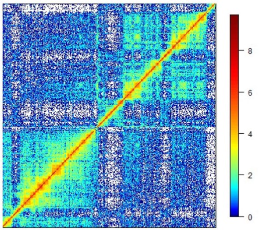
Log-transformed contact matrix |$\log(C)$|. White color corresponds to |$C_{ij} = 0$| or, equivalently, |$\log(C_{ij}) = -\infty$|.
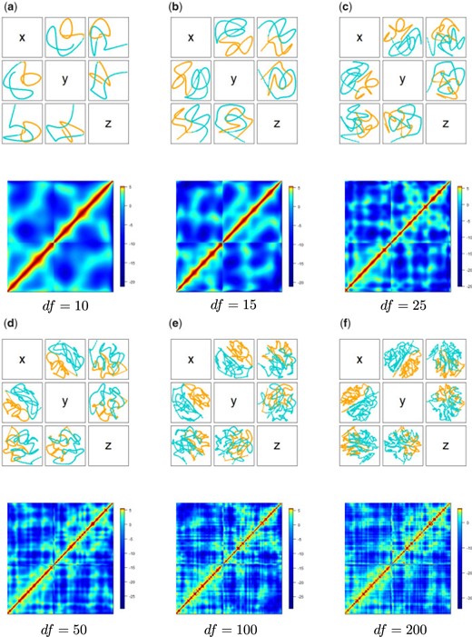
|$\hat X_{df}$|, the projections of the resulting reconstruction, with colors (orange, teal) distinguishing chromosome arms, and |$- D^2(\hat{X}_{df})+\beta$|, the approximation of |$\log(C)$|, obtained via PoisMS for differing degrees-of-freedom values |$df$|.
Many approaches have been proposed to tackle this problem with broad distinction between optimization and model-based methods (Varoquaux and others, 2014; Rieber and Mahony, 2017). A common first step is conversion of the contact matrix into a distance matrix |$\mathcal D=[\mathcal D_{ij}]$| (Duan and others, 2010; Varoquaux and others, 2014; Ay and others, 2014; Shavit and others, 2014), followed by solving the MDS (Hastie and others, 2009) problem: position points (corresponding to genomic loci) in 3D so that the resultant interpoint distances best conform to the distance matrix.
A variety of methods have also been used for transforming contacts to distances. At one extreme, in terms of imposing biological assumptions, are methods that relate observed intra-chromosomal contacts to genomic distances and then ascribe physical distances based on organism specific findings on chromatin packing (Duan and others, 2010) or relationships between genomic and physical distances for crumpled polymers (Ay and others, 2014). Such distances inform the subsequent optimization step as they permit incorporation of known biological constraints that can be expressed in terms of physical separation. Importantly, these constraints include prescriptions on the 3D separation between contiguous genomic bins. It is by this means that obtaining a 1D curve is indirectly facilitated. However, obtaining physical distances requires both strong assumptions and organism specific data (Fudenberg and Mirny, 2012). More broadly, a number of approaches (Zhang and others, 2013; Varoquaux and others, 2014; Zou and others, 2016; Rieber and Mahony, 2017) utilize power-law transfer functions to map contacts to (non-physical) distances
Here, common choices for the weights |$\mathcal W_{ij}$| include |$\mathcal D_{ij}^{-1}$| (Zhang and others, 2013) and |$\mathcal D_{ij}^{-2}$| (Varoquaux and others, 2014), these being analogous to precision weighting since large |$C_{ij}$| (small |$\mathcal D_{ij}$|) are more accurately measured. Similarly, the penalty (second) term maximizes the pairwise distances for loci bins with |$C_{ij} = 0$| under the presumption that such loci should not be too close.
It is worth noting that (2.1), and related criteria, correspond to a nonconvex, nonlinear optimization problem that is NP hard and while various devices have been employed to mitigate the computational burden (e.g., Zhang and others, 2013), computational concerns, particularly for high resolution (many loci bins) problems, remain forefront.
Probabilistic methods model the contact counts with an optimization goal of maximizing the corresponding log-likelihood.
In particular, Poisson models, |$C_{ij} \sim Pois(\lambda_{ij})$|, are widely used (Varoquaux and others, 2014; Zou and others, 2016, Park and Lin, 2017), where |$\lambda_{ij} = \lambda_{ij}(x_1,\ldots,x_n)$| is a function of the genomic loci spatial coordinates |$x_1,\ldots,x_n$|. For example, Rosenthal and others (2019) prescribe exponential dependence between the Poisson rate parameter and inter-loci distances: |$\lambda_{ij} = \beta\|x_i - x_j\|^\alpha$| for some |$\alpha<0$|, a framework we slightly modify in Section 2.6.
All existing approaches implicitly represent chromatin as a polygonal chain. Constraints on the geometrical structure of the polygonal chain can be imposed via penalties on edge lengths and angles between successive edges, with even quaternion-based formulations employed (Caudai and others, 2015). Rosenthal and others (2019) utilize penalties to control smoothness of the resulting conformations. However, despite imparting targeted properties to the resulting reconstruction, such penalty-based approaches increase the complexity of the objective, its gradient and Hessian, both slowing and limiting, especially with respect to resolution, associated algorithms.
Here, we develop a suite of novel approaches that directly model chromatin configuration as a 1D curve in 3D. Our primary method, Poisson Metric Scaling (PoisMS), is based on a Poisson model for contact counts and provides an efficient means for obtaining smooth 1D reconstructions, that combines advantages of both MDS and probabilistic models. This technique utilizes two building blocks of intrinsic interest. First, we introduce the PCMS approach that features an optimization problem inspired by MDS and stated in terms of inner products. This problem admits a simple solution obtained via the singular value decomposition. Next, we develop WPCMS, a weighted version of PCMS that, importantly, models distances rather than inner products and further permits control over the influence of particular elements of the contact matrix on the resulting reconstruction. This technique requires an iterative algorithm that uses PCMS as the core component. Finally, WPCMS in turn can be used in conjunction with projected gradient descent (PGD) to solve a second-order approximation of the Poisson log-likelihood, yielding our PoisMS algorithm.
2.2. PCMS: metric scaling with a smooth curve constraint
The PCMS technique is based on classical MDS. Given a symmetric matrix |$Z$|, PCMS treats it as a similarity matrix and approximates it by an inner product matrix (Buja and others, 2008). In particular, |$Z$| can correspond to the contact matrix after conversion to a distance matrix followed by double centering, the standard MDS device that turns (Euclidean) squared distances into inner products. We illustrate this approach in the Section S2 of the Supplementary material available at Biostatistics online with distances obtained via power-law transformation. However, while it is thereby possible to use PCMS as a standalone reconstruction tool, we seek methods that avoid having to convert contacts to distances. So, here we develop PCMS with a view to utilizing it as a building block of our PoisMS technique.
Hereafter, we denote the corresponding solution by |$\hat\Theta = \operatorname{PCMS}(Z, H)$|, the resulting chromatin reconstruction by |$\hat X = H\hat\Theta$| and the approximation of the original matrix |$Z$| as |$\hat Z = S(\hat X)$|.
2.3. PCMS solution via eigen-decomposition
Note that the parameter |$\Theta$| in the PCMS problem (2.5) is unconstrained. Since |$\Theta$| is defined up to a multiplication by a full-rank matrix, we can assume |$H$| to be a matrix with orthogonal columns. To find the PCMS solution the following lemma, proved in Section S1 of the Supplementary material available at Biostatistics online, is useful.
The computational efficiency of PCMS derives from the fact that it relies on eigen-decomposition of a small |$k \times k$| matrix, requiring only |$O(k^3)$| additional operations.
2.4. WPCMS: a distance-based model for chromatin reconstruction
As indicated, direct application of PCMS to Hi-C data is limited by the need to convert contact counts to distances and then (via double centering) to inner products since such conversion can be problematic. Even simplistic approaches, based on power-law transformation, prescribe a value for the index parameter, failing to accommodate dependence of the index on influencing factors such as cell type, chromosome, organism, and resolution. Moreover, the double centering trick requires that resultant distances be Euclidean.
Accordingly, we develop a distance-based version of PCMS, wherein the symmetric matrix |$Z$| contains pairwise squared distances, as opposed to inner products. Additional flexibility is facilitated by introducing weights to the problem setup, which permits control over the impact of particular elements |$Z_{ij}$| on the reconstruction, for example to counteract diagonal dominance (Yang and others, 2017). Although the resulting technique, Weighted PCMS (WPCMS), can again be used as a standalone reconstruction tool (Section S5 of the Supplementary material available at Biostatistics online), akin to PCMS its primary purpose is as component of the PoisMS approach.
The corresponding solution and reconstruction are denoted by |$\hat\Theta=\operatorname{PCMS}_{W}(Z, H)$| and |$\hat X = H\hat \Theta$|, respectively, along with the corresponding approximation |$\hat Z = D^2(\hat X)$| of matrix |$Z$|.
2.5. Iterative algorithm for solving the WPCMS problem
Here |$\operatorname{proj}_{\mathcal{M}(H)}(S)$| denotes the projection of matrix |$S$| onto the matrix manifold |$\mathcal{M}(H)$|. The [Gradient] step makes recourse to the following Lemma, proved in Section S3 of the Supplementary material available at Biostatistics online.
Let |$D^2$| denote the matrix of squared distances corresponding to inner product matrix |$S$| (as in 2.9). If |$G =W * \left(Z - D^2\right)$| and |$G_+ = \operatorname{diag}(G \cdot \mathbf{1})$| is the diagonal matrix containing row sums of |$G$| on the diagonal, then up to a scaling factor |$\nabla\ell_{\rm WPCMS}(S) = G - G_+.$|
(1) [Initialize] Generate random |$\Theta\in\mathbb{R}^{k\times 3}$|, set the reconstruction |$X =H \Theta$|.
(2) Repeat until convergence:
[2.1] [SDG] Calculate the current guess for the inner product matrix |$S = XX^T$| and use it to compute the matrix of squared distances |$D^2 = \operatorname{diag}(S)\cdot\mathbf{1}^T + \mathbf{1}\cdot\operatorname{diag}(S)^T - 2S.$| Then compute |$G =W * \left(Z - D^2\right)$| as well as |$G_+ = \operatorname{diag}(G \cdot \mathbf{1})$|.
[2.2] [Gradient] Update matrix of inner products |$S: = S - (G - G_+).$|
[2.3] [Projection] Update spline coefficients using PCMS |$\Theta:=~\operatorname{PCMS}(S, H)$|, then update the reconstruction |$X =~H \Theta$|.
Convergence is assessed via the stopping criterion |$\left|\frac{\ell_{\rm WPCMS}(\Theta_{old})-\ell_{\rm WPCMS}(\Theta_{new})}{\ell_{\rm WPCMS}(\Theta_{old})}\right|<\epsilon_1,$| where |$\epsilon_1$| is a pre-chosen accuracy rate, and |$\Theta_{\rm old}$| and |$\Theta_{\rm new}$| are |$\Theta$| values calculated at the previous and current iterations respectively. Details and extensions of WPCMS are provided in the Sections S4 and S6 of the Supplementary material available at Biostatistics online.
2.6. PoisMS: Poisson model for contact counts
In (2.11), we use squared distance rather than distance, reflecting criterion (2.1) and conferring computational convenience. We denote the corresponding matrix of spline coefficients by |$\hat\Theta =~ \operatorname{PoisMS}(C, H)$| and the resulting chromatin reconstruction by |$\hat X = H\hat \Theta$|.
2.7. Iterative algorithm for solving PoisMS problem
A virtue of the Poisson model is that the second-order Taylor approximation (SOA) of the negative log-likelihood (2.12) is simply the weighted Frobenius norm. Further, it is well known that the optimal value of this SOA amounts to one step of the Newton method for optimizing the original loss function. We use these facts to develop an iterative algorithm based on the WPCMS technique, which is equivalent to a projected Newton Method.
Here |$*$| is the Hadamard (element-wise) product, with matrix exponentiation and division also being interpreted as element-wise operations.
The last step of our PoisMS algorithm is to update |$\beta$| according to the current guess of |$\Theta$|. This can be done by optimizing the negative log-likelihood with respect to |$\beta$|. All together this leads to the following algorithm that repeatedly approximates the Poisson objective at current guess |$\Theta$| by a quadratic function and shifts |$\Theta$| towards the global minimum of this quadratic approximation:
(1) [Initialize] Generate random |$\Theta\in\mathbb{R}^{k\times 3}$|, set the reconstruction |$X = H\Theta$|.
(2) Repeat until convergence:
[2.1] [Update |$\beta$|] Update the intercept |$\beta := \log\left(\frac {\sum_{1 \leq i,j \leq n} C_{ij} }{\sum_{1 \leq i,j \leq n} e^{- \|x_i-x_j\|^2} }\right)$|.
[2.2][SOA] Calculate SOA matrices |$W = e^{- D^2(X) + \beta}$| and |$Z = D^2(X) - \frac {C -W} {W}.$|
[2.3] [WPCMS] Update the spline coefficients using WPCMS approach |$\Theta := \operatorname{PCMS}_W(Z, H)$|, then update the reconstruction |$X = H\Theta$|.
The stopping rule for the PoisMS algorithm is similar to WPCMS: for some fixed accuracy rate |$\epsilon_2$| we check if the updated |$(\Theta_{\rm new}, \beta_{\rm new})$| meets the criteria |$\left|\frac{\ell_{\rm PoisMS}(\Theta_{\rm old}, \beta_{\rm old})-\ell_{PoisMS}(\Theta_{\rm new}, \beta_{\rm new})}{\ell_{\rm PoisMS}(\Theta_{\rm old}, \beta_{\rm old})}\right|<~\epsilon_2$| after each iteration of steps 2.1–2.3.
The nonconvexity of the PoisMS criteria (2.13) implies that initialization can impact the resulting reconstruction. In the Sections S7–S10 of the Supplementary material available at Biostatistics online, we discuss use of WPCMS to provide a warm start for the PoisMS algorithm, as well as algorithmic extensions and computational complexity.
2.8. Determination of principal curve degrees-of-freedom
Initially, we tried cross-validation to find the optimal value of |$df$|, as is common for smoothing (penalty) parameter determination. However, the complex and structural dependencies that characterize contact matrices made this approach problematic. As an alternative we adopted an approach based on identifying the “elbow" that is prototypic in graphs of resubstitution error, here |${\rm err}(\hat X_{df}, \hat \beta_{df})$|, versus model complexity, here |$df$|. The logic as to why this change point constitutes a basis for model complexity determination is described in Breiman and others (1984) in terms of bias-variance tradeoff. Elbow identification is also used for determining appropriate numbers of principal components (Jolliffe, 2002) and clusters (Hastie and others, 2009), as well as dimension in MDS (Kruskal and Wish, 1978) and non-negative matrix factorization (see Hutchins and others, 2008) problems.
2.9. Accuracy assessment via multiplex fluorescence in situ hybridization
While the prescription in Section 2.8 provides a means for selecting a particular PoisMS model, it does not address the accuracy of the chosen model. The absence of gold standards makes such assessment challenging. In comparing competing 3D genome reconstructions several authors have appealed to simulation (Zhang and others, 2013; Varoquaux and others, 2014; Zou and others, 2016; Park and Lin, 2017), however, real data referents are preferable. To that end, many of the same reconstruction algorithm developers have made recourse to fluorescence in situ hybridization (FISH) imaging as a basis for gauging accuracy. This proceeds by comparing distances between imaged probes with corresponding reconstruction-based distances. But such methods are necessarily limited by the sparse number of probes (|$\sim$|2–6; see Lieberman-Aiden and others, 2009; Shavit and others, 2014; Park and Lin, 2017) and the modest resolution thereof, many straddling over 1 megabase. The recent advent of multiplex FISH (Wang and others, 2016) transforms 3D genome reconstruction accuracy evaluation by providing an order of magnitude more probes and hence two orders of magnitude more inter-probe distances than conventional FISH. Moreover, the probes are at higher resolution and centered at topologically associated domains (see Dixon and others, 2012). We use this imaging data, along with companion accuracy assessment approaches (Segal and Bengtsson, 2018) to evaluate our PoisMS reconstructions.
The image-based 3D genomic coordinates furnished from multiplex FISH serve to define the gold standard by which we assess reconstructions. The existence of numerous multiplex FISH replicates is crucial for this task and three steps are necessary to effect such evaluation.
2.9.1. Obtaining the gold standard
2.9.2. Computing the reference distribution
Treating the average Procrustes conformation |$\bar M$| as our gold standard we obtain a reference distribution by measuring the dissimilarity between it and the multiplex FISH replicates: |$d(\bar M, M_i).$| The resulting empirical distribution captures experimental variation around the gold standard. A fine point is that this distribution will exhibit reduced dispersion compared to its target population quantity owing to data re-use since |$M_i$| contributes to |$\bar M$|. While this concern could be mitigated by employing leave-one-out techniques the large number of available replicates (|$>$|110) renders this unnecessary (Segal and Bengtsson, 2018).
2.9.3. Evaluating chromatin reconstructions
To evaluate reconstructions resulting from the PoisMS approach we first need to align the reconstruction with the gold standard. This may involve preliminary coarsening of one or other coordinate sets to yield comparable resolution. Here, the genomic coordinate ranges for each multiplex FISH probe are coarser than the Hi-C bins used in our reconstructions. So, we calculate the average of the reconstruction coordinates falling in the corresponding multiplex FISH bins to obtain a lower resolution reconstruction |$\hat X$| of the same dimension as |$\bar M$|. To quantify how close this reconstruction is to the gold standard |$\bar M$|, we again measure dissimilarity following alignment |$d(\bar M,\hat X).$| Interpretations of this quantity in the context of the reference distribution are presented in the Section 3.
2.10. A contrasting reconstruction algorithm: HSA
To compare our PoisMS solution with an alternate reconstruction algorithm we make recourse to HSA (Zou and others, 2016). This technique provides an interesting contrast in that it employs a similar Poisson formulation to (2.12) but instead of contiguity being captured via principal curves per (2.4), it is indirectly imparted by constraints that induce dependencies on a hidden Gaussian Markov chain over the solution coordinates. Obtaining these spatial coordinates is achieved via simulated annealing with further smoothness effected via distance-based penalization.
HSA has performed well in some benchmarking studies and features several compelling attributes including (i) simultaneously handling multiple data tracks allowing for integration of replicate contact maps and (ii) adaptively estimating the power-law index whereby contacts are transformed to distances as previously emphasized. Nonetheless, in contrast to PoisMS, HSA incurs a substantial compute and memory burden, and questions surrounding robustness have been raised (Rieber and Mahony, 2017).
To compare PoisMS performance with HSA we use the approach described in Section 2.9. Having obtained a HSA reconstruction we measure the dissimilarity between the reconstruction and the gold standard. The quantity so obtained is interpreted in the context of the attendant reference distribution (see Section 3.3).
3. Results
3.1. Chromosome reconstructions
We present PoisMS reconstructions for IMR90 cell chromosome 20 at 100kb resolution for which multiplex FISH and Hi-C data acquisition and processing has been previously described (Segal and Bengtsson, 2018). Results for chromosome 21 are presented in the section S11 of the Supplementary material available at Biostatistics online.
In Figure 1, we present the heatmap for |$\log(C)$|. The resulting PoisMS reconstructions |$\hat X_{df}$| along with the Poisson parameter matrix |$\log(\Lambda_{df}) = - D^2(\hat X_{df}) + \beta$|, that can be viewed as an approximation of |$\log(C)$|, are presented in Figure 2 for a series of degrees-of-freedom values.
3.2. Determining degrees-of-freedom
The graph of error rate |$err(\hat X_{df}, \hat \beta_{df})$| versus |$df$| reveals rapidly decreasing error rates up to |$df = 30$| with subsequent gradual decline (Figure 3). The optimal |$df$| according to the elbow heuristic, obtained using the R package segmented (Muggeo, 2008), is |$df = 25$|, also shown in Figure 3.
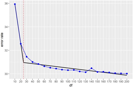
Error rate |$err(\hat X_{df}, \hat\beta_{df})$| vs. degrees-of-freedom |$df$| plot for the PoisMS approach. The segmented regression is given by the piecewise linear fit (black) with the degrees-of-freedom selected via kink estimation indicated by the red vertical line and segmentation change point corresponding to |$df = 25$|.
3.3. Evaluating reconstructions via the multiplex FISH referent
Procrustes alignment of 3D conformations, and calculation of the corresponding distances |$d_{\rm proc}(\cdot,\cdot)$|, was performed using the R package vegan (Oksanen and others, 2019). We obtain the multiplex FISH medoid conformation based on the smallest row sum (2.17) of the dissimilarity matrix of normalized Procrustes distances (2.16) as described above. The |$111$| multiplex FISH replicate conformations are then aligned to the medoid as a prelude to calculating the average Procrustes conformation—our gold standard. Figure 4 shows the histogram of dissimilarities between multiplex FISH replicates and our derived gold standard that constitutes the reference distribution. We position the PoisMS reconstruction dissimilarities therein corresponding to the indicated series of degrees-of-freedom values. HSA reconstruction dissimilarity values are also included.
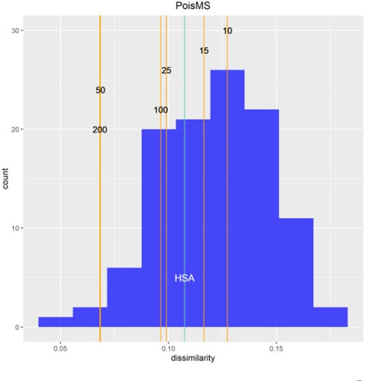
Reference distribution measuring the dissimilarity between the gold standard |$\bar M$| and 111 multiplex FISH replicate conformations |$M_i$| for chromosome 20. The vertical orange lines correspond to the dissimilarity between |$\bar M$| and the low-resolution reconstruction |$\hat X_{df}$| calculated via PoisMS for different |$df$| values; the light blue line corresponds to the HSA reconstruction (see Sections 2.9 and 2.10).
The following conclusions can be drawn from Figure 4. For chromosome 20 (see the Section S11 of the Supplementary material available at Biostatistics online for chromosome 21), all fits for PoisMS lie within the range of the multiplex FISH dissimilarity distribution that reflects experimental variation. The fact that the PoisMS dissimilarity values are in the left tail of this distribution indicates the accuracy of the proposed reconstructions, highlighting the utility of the proposed methodology. Further, that larger dissimilarity values pertain for HSA, particularly for chromosome 21, suggests that PoisMS performs at least comparably to this well benchmarked alternative. That PoisMS wall clock times are minutes rather than days for HSA is notable.
4. Discussion
Central to our principal curve based approaches to 3D chromatin reconstruction is that the configuration of an individual chromosome within the nucleus can be treated as a contiguous 1D curve since the diameter of the chromatin fiber is negligible compared to the nuclear volume. The extent to which the curve is “smooth” is determined by an adaptively selected degrees-of-freedom parameter. As mentioned in Section 1, previous reconstruction methods either impart contiguity indirectly by prescribing constraints, which are difficult to specify, or impose it post hoc. In comparison, our methods based on principal curves are computationally efficient, readily scale to high resolution contact data and are parsimonious with regard tuning parameters.
Our implementation of PoisMS utilizes cubic spline basis functions, which contribute to this computational efficiency. However, the nature of chromatin folding and attendant Hi-C data is such that these bases will be less effective in capturing fine 3D structure, as opposed to global backbone architecture. This derives from the hierarchical, domain-based organization of chromatin, aspects that have been tackled by some reconstruction algorithms using strategies that synthesize solutions obtained at differing scales (Rieber and Mahony, 2017; Trieu and others, 2019). We will investigate whether principal curve solutions can similarly serve as building blocks in addition to exploring the use of alternate basis functions, notably wavelets.
Our analyses of Hi-C data from IMR90 cells was motivated by the availability of corresponding multiplex FISH data enabling accuracy assessment. However, the extent and resolution of multiplex FISH imaging is limited, narrowing the applicability of this means of evaluation. An even more fundamental issue pertains to attempting chromatin reconstruction using bulk Hi-C data from large cell populations. As has been emphasized (Lando and others, 2018), the presence of numerous conflicting contacts suggests that the notion of a consensus underlying 3D conformation is questionable and that there is substantial cell-to-cell structural variation. This places a premium on pursuing single-cell reconstructions as enabled by the recent emergence of single-cell Hi-C protocols (Ramani and others, 2017). That one of these advances (Stevens and others, 2017) also provides parallel imaging data, putatively enabling reconstruction accuracy determination, underscores the importance of applying reconstruction methods in single-cell settings, despite contact map sparsity, and is the subject of future work.
5. Software
Proposed methods are implemented in the R package PoisMS; the software is available from Github (https://github.com/ElenaTuzhilina/PoisMS).
Supplementary material
Supplementary material is available online at http://biostatistics.oxfordjournals.org.
Funding
National Institutes of Health (GM-109457 to M.S.), in part; National Science Foundation (DMS-2013736 and IIS 1837931 to T.J.H.), in part; and National Institutes of Health (5R01 EB 001988-21).
Acknowledgments
The authors thank the Associate Editor and two reviewers for very helpful comments, including critical appraisal of our original approach, which led to substantial improvements in methodology.
Conflict of Interest: None declared.
